Mastering Elasticsearch, Second Edition (2015)
Chapter 2. Power User Query DSL
In the previous chapter, we looked at what Apache Lucene is, how its architecture looks, and how the analysis process is handled. In addition to these, we saw what Lucene query language is and how to use it. We also discussed Elasticsearch, its architecture, and core concepts. In this chapter, we will dive deep into Elasticsearch focusing on the Query DSL. We will first go through how Lucene scoring formula works before turning to advanced queries. By the end of this chapter, we will have covered the following topics:
· How the default Apache Lucene scoring formula works
· What query rewrite is
· What query templates are and how to use them
· How to leverage complicated Boolean queries
· What are the performance implications of large Boolean queries
· Which query you should use for your particular use case
Default Apache Lucene scoring explained
A very important part of the querying process in Apache Lucene is scoring. Scoring is the process of calculating the score property of a document in a scope of a given query. What is a score? A score is a factor that describes how well the document matched the query. In this section, we'll look at the default Apache Lucene scoring mechanism: the TF/IDF (term frequency/inverse document frequency) algorithm and how it affects the returned document. Knowing how this works is valuable when designing complicated queries and choosing which queries parts should be more relevant than the others. Knowing the basics of how scoring works in Lucene allows us to tune queries more easily and the results retuned by them to match our use case.
When a document is matched
When a document is returned by Lucene, it means that it matched the query we've sent. In such a case, the document is given a score. Sometimes, the score is the same for all the documents (like for the constant_score query), but usually this won't be the case. The higher the score value, the more relevant the document is, at least at the Apache Lucene level and from the scoring formula point of view. Because the score is dependent on the matched documents, query, and the contents of the index, it is natural that the score calculated for the same document returned by two different queries will be different. Because of this, one should remember that not only should we avoid comparing the scores of individual documents returned by different queries, but we should also avoid comparing the maximum score calculated for different queries. This is because the score depends on multiple factors, not only on the boosts and query structure, but also on how many terms were matched, in which fields, the type of matching that was used on query normalization, and so on. In extreme cases, a similar query may result in totally different scores for a document, only because we've used a custom score query or the number of matched terms increased dramatically.
For now, let's get back to the scoring. In order to calculate the score property for a document, multiple factors are taken into account, which are as follows:
· Document boost: The boost value given for a document during indexing.
· Field boost: The boost value given for a field during querying.
· Coord: The coordination factor that is based on the number of terms the document has. It is responsible for giving more value to the documents that contain more search terms compared to other documents.
· Inverse document frequency: Term-based factor telling the scoring formula how rare the given term is. The higher the inverse document frequency, the rarer the term is. The scoring formula uses this factor to boost documents that contain rare terms.
· Length norm: A field-based factor for normalization based on the number of terms given field contains (calculated during indexing and stored in the index). The longer the field, the lesser boost this factor will give, which means that the Apache Lucene scoring formula will favor documents with fields containing lower terms.
· Term frequency: Term-based factor describing how many times a given term occurs in a document. The higher the term frequency, the higher the score of the document will be.
· Query norm: Query-based normalization factor that is calculated as a sum of a squared weight of each of the query terms. Query norm is used to allow score comparison between queries, which, as we said, is not always easy and possible.
TF/IDF scoring formula
Since the Lucene version 4.0, contains different scoring formulas and you are probably aware of them. However, we would like to discuss the default TF/IDF formula in greater detail. Please keep in mind that in order to adjust your query relevance, you don't need to understand the following equations, but it is very important to at least know how it works as it simplifies the relevancy tuning process.
Lucene conceptual scoring formula
The conceptual version of the TF/IDF formula looks as follows:

The presented formula is a representation of a Boolean Model of Information Retrieval combined with a Vector Space Model of Information Retrieval. Let's not discuss this and let's just jump into the practical formula, which is implemented by Apache Lucene and is actually used.
Note
The information about the Boolean Model and Vector Space Model of Information Retrieval are far beyond the scope of this book. You can read more about it at http://en.wikipedia.org/wiki/Standard_Boolean_model andhttp://en.wikipedia.org/wiki/Vector_Space_Model.
Lucene practical scoring formula
Now, let's look at the following practical scoring formula used by the default Apache Lucene scoring mechanism:

As you can see, the score factor for the document is a function of query q and document d, as we have already discussed. There are two factors that are not dependent directly on query terms, coord and queryNorm. These two elements of the formula are multiplied by the sum calculated for each term in the query.
The sum, on the other hand, is calculated by multiplying the term frequency for the given term, its inverse document frequency, term boost, and the norm, which is the length norm we've discussed previously.
Sounds a bit complicated, right? Don't worry, you don't need to remember all of that. What you should be aware of is what matters when it comes to document score. Basically, there are a few rules, as follows, which come from the previous equations:
· The rarer the matched term, the higher the score the document will have. Lucene treats documents with unique words as more important than the ones containing common words.
· The smaller the document fields (contain less terms), the higher the score the document will have. In general, Lucene emphasizes shorter documents because there is a greater possibility that those documents are exactly about the topic we are searching for.
· The higher the boost (both given during indexing and querying), the higher the score the document will have because higher boost means more importance of the particular data (document, term, phrase, and so on).
As we can see, Lucene will give the highest score for the documents that have many uncommon query terms matched in the document contents, have shorter fields (less terms indexed), and will also favor rarer terms instead of the common ones.
Note
If you want to read more about the Apache Lucene TF/IDF scoring formula, please visit Apache Lucene Javadocs for the TFIDFSimilarity class available at http://lucene.apache.org/core/4_9_0/core/org/apache/lucene/search/similarities/TFIDFSimilarity.html.
Elasticsearch point of view
On top of all this is Elasticsearch that leverages Apache Lucene and thankfully allows us to change the default scoring algorithm by specifying one of the available similarities or by implementing your own. But remember, Elasticsearch is more than just Lucene because we are not bound to rely only on Apache Lucene scoring.
We have different types of queries, where we can strictly control how the score of the documents is calculated, for example, by using the function_score query, we are allowed to use scripting to alter score of the documents; we can use the rescore functionality introduced in Elasticsearch 0.90 to recalculate the score of the returned documents, by another query run against top N documents, and so on.
Note
For more information about the queries from Apache Lucene point of view, please refer to Javadocs, for example, the one available at http://lucene.apache.org/core/4_9_0/queries/org/apache/lucene/queries/package-summary.html.
An example
Till now we've seen how scoring works. Now we would like to show you a simple example of how the scoring works in real life. To do this, we will create a new index called scoring. We do that by running the following command:
curl -XPUT 'localhost:9200/scoring' -d '{
"settings" : {
"index" : {
"number_of_shards" : 1,
"number_of_replicas" : 0
}
}
}'
We will use an index with a single physical shard and no replicas to keep it as simple as it can be (we don't need to bother about distributed document frequency in such a case). Let's start with indexing a very simple document that looks as follows:
curl -XPOST 'localhost:9200/scoring/doc/1' -d '{"name":"first document"}'
Let's run a simple match query that searches for the document term:
curl -XGET 'localhost:9200/scoring/_search?pretty' -d '{
"query" : {
"match" : { "name" : "document" }
}
}'
The result returned by Elasticsearch would be as follows:
{
"took" : 1,
"timed_out" : false,
"_shards" : {
"total" : 1,
"successful" : 1,
"failed" : 0
},
"hits" : {
"total" : 1,
"max_score" : 0.19178301,
"hits" : [ {
"_index" : "scoring",
"_type" : "doc",
"_id" : "1",
"_score" : 0.19178301,
"_source":{"name":"first document"}
} ]
}
}
Of course, our document was matched and it was given a score. We can also check how the score was calculated by running the following command:
curl -XGET 'localhost:9200/scoring/doc/1/_explain?pretty' -d '{
"query" : {
"match" : { "name" : "document" }
}
}'
The results returned by Elasticsearch would be as follows:
{
"_index" : "scoring",
"_type" : "doc",
"_id" : "1",
"matched" : true,
"explanation" : {
"value" : 0.19178301,
"description" : "weight(name:document in 0) [PerFieldSimilarity], result of:",
"details" : [ {
"value" : 0.19178301,
"description" : "fieldWeight in 0, product of:",
"details" : [ {
"value" : 1.0,
"description" : "tf(freq=1.0), with freq of:",
"details" : [ {
"value" : 1.0,
"description" : "termFreq=1.0"
} ]
}, {
"value" : 0.30685282,
"description" : "idf(docFreq=1, maxDocs=1)"
}, {
"value" : 0.625,
"description" : "fieldNorm(doc=0)"
} ]
} ]
}
}
As we can see, we've got detailed information on how the score has been calculated for our query and the given document. We can see that the score is a product of the term frequency (which is 1 in this case), the inverse document frequency (0.30685282), and the field norm (0.625).
Now, let's add another document to our index:
curl -XPOST 'localhost:9200/scoring/doc/2' -d '{"name":"second example document"}'
If we run our initial query again, we will see the following response:
{
"took" : 6,
"timed_out" : false,
"_shards" : {
"total" : 1,
"successful" : 1,
"failed" : 0
},
"hits" : {
"total" : 2,
"max_score" : 0.37158427,
"hits" : [ {
"_index" : "scoring",
"_type" : "doc",
"_id" : "1",
"_score" : 0.37158427,
"_source":{"name":"first document"}
}, {
"_index" : "scoring",
"_type" : "doc",
"_id" : "2",
"_score" : 0.2972674,
"_source":{"name":"second example document"}
} ]
}
}
We can now compare how the TF/IDF scoring formula works in real life. After indexing the second document to the same shard (remember that we created our index with a single shard and no replicas), the score changed, even though the query is still the same. That's because different factors changed. For example, the inverse document frequency changed and thus the score is different. The other thing to notice is the scores of both the documents. We search for a single word (the document), and the query match was against the same term in the same field in case of both the documents. The reason why the second document has a lower score is that it has one more term in the name field compared to the first document. As you will remember, we already know that Lucene will give a higher score to the shorter documents.
Hopefully, this short introduction will give you better insight into how scoring works and will help you understand how your queries work when you are in need of relevancy tuning.
Query rewrite explained
We have already talked about scoring, which is valuable knowledge, especially when trying to improve the relevance of our queries. We also think that when debugging your queries, it is valuable to know how all the queries are executed; therefore, it is because of this we decided to include this section on how query rewrite works in Elasticsearch, why it is used, and how to control it.
If you have ever used queries, such as the prefix query and the wildcard query, basically any query that is said to be multiterm, you've probably heard about query rewriting. Elasticsearch does that because of performance reasons. The rewrite process is about changing the original, expensive query to a set of queries that are far less expensive from Lucene's point of view and thus speed up the query execution. The rewrite process is not visible to the client, but it is good to know that we can alter the rewrite process behavior. For example, let's look at what Elasticsearch does with a prefix query.
Prefix query as an example
The best way to illustrate how the rewrite process is done internally is to look at an example and see what terms are used instead of the original query term. Let's say we have the following data in our index:
curl -XPUT 'localhost:9200/clients/client/1' -d '{
"id":"1", "name":"Joe"
}'
curl -XPUT 'localhost:9200/clients/client/2' -d '{
"id":"2", "name":"Jane"
}'
curl -XPUT 'localhost:9200/clients/client/3' -d '{
"id":"3", "name":"Jack"
}'
curl -XPUT 'localhost:9200/clients/client/4' -d '{
"id":"4", "name":"Rob"
}'
We would like to find all the documents that start with the j letter. As simple as that, we run the following query against our clients index:
curl -XGET 'localhost:9200/clients/_search?pretty' -d '{
"query" : {
"prefix" : {
"name" : {
"prefix" : "j",
"rewrite" : "constant_score_boolean"
}
}
}
}'
We've used a simple prefix query; we've said that we would like to find all the documents with the j letter in the name field. We've also used the rewrite property to specify the query rewrite method, but let's skip it for now, as we will discuss the possible values of this parameter in the later part of this section.
As the response to the previous query, we've got the following:
{
"took" : 2,
"timed_out" : false,
"_shards" : {
"total" : 5,
"successful" : 5,
"failed" : 0
},
"hits" : {
"total" : 3,
"max_score" : 1.0,
"hits" : [ {
"_index" : "clients",
"_type" : "client",
"_id" : "3",
"_score" : 1.0,
"_source":{
"id":"3", "name":"Jack"
}
}, {
"_index" : "clients",
"_type" : "client",
"_id" : "2",
"_score" : 1.0,
"_source":{
"id":"2", "name":"Jane"
}
}, {
"_index" : "clients",
"_type" : "client",
"_id" : "1",
"_score" : 1.0,
"_source":{
"id":"1", "name":"Joe"
}
} ]
}
}
As you can see, in response we've got the three documents that have the contents of the name field starting with the desired character. We didn't specify the mappings explicitly, so Elasticsearch has guessed the name field mapping and has set it to string-based and analyzed. You can check this by running the following command:
curl -XGET 'localhost:9200/clients/client/_mapping?pretty'
Elasticsearch response will be similar to the following code:
{
"client" : {
"properties" : {
"id" : {
"type" : "string"
},
"name" : {
"type" : "string"
}
}
}
}
Getting back to Apache Lucene
Now let's take a step back and look at Apache Lucene again. If you recall what Lucene inverted index is built of, you can tell that it contains a term, a count, and a document pointer (if you can't recall, please refer to the Introduction to Apache Lucene section inChapter 1, Introduction to Elasticsearch). So, let's see how the simplified view of the index may look for the previous data we've put to the clients index, as shown in the following figure:
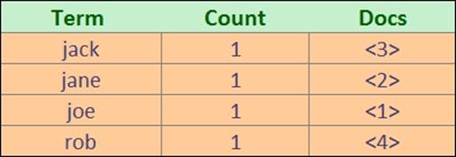
What you see in the column with the term text is quite important. If we look at Elasticsearch and Apache Lucene internals, you can see that our prefix query was rewritten to the following Lucene query:
ConstantScore(name:jack name:jane name:joe)
We can check the portions of the rewrite using the Elasticsearch API. First of all, we can use the Explain API by running the following command:
curl -XGET 'localhost:9200/clients/client/1/_explain?pretty' -d '{
"query" : {
"prefix" : {
"name" : {
"prefix" : "j",
"rewrite" : "constant_score_boolean"
}
}
}
}'
The result would be as follows:
{
"_index" : "clients",
"_type" : "client",
"_id" : "1",
"matched" : true,
"explanation" : {
"value" : 1.0,
"description" : "ConstantScore(name:joe), product of:",
"details" : [ {
"value" : 1.0,
"description" : "boost"
}, {
"value" : 1.0,
"description" : "queryNorm"
} ]
}
}
We can see that Elasticsearch used a constant score query with the joe term against the name field. Of course, this is on Lucene level; Elasticsearch actually used a cache to get the terms. We can see this by using the Validate Query API with a command that looks as follows:
curl -XGET 'localhost:9200/clients/client/_validate/query?explain&pretty' -d '{
"query" : {
"prefix" : {
"name" : {
"prefix" : "j",
"rewrite" : "constant_score_boolean"
}
}
}
}'
The result returned by Elasticsearch would look like the following:
{
"valid" : true,
"_shards" : {
"total" : 1,
"successful" : 1,
"failed" : 0
},
"explanations" : [ {
"index" : "clients",
"valid" : true,
"explanation" : "filtered(name:j*)->cache(_type:client)"
} ]
}
Query rewrite properties
Of course, the rewrite property of multiterm queries can take more than a single constant_score_boolean value. We can control how the queries are rewritten internally. To do that, we place the rewrite parameter inside the JSON object responsible for the actual query, for example, like the following code:
{
"query" : {
"prefix" : {
"name" : "j",
"rewrite" : "constant_score_boolean"
}
}
}
The rewrite property can take the following values:
· scoring_boolean: This rewrite method translates each generated term into a Boolean should clause in a Boolean query. This rewrite method causes the score to be calculated for each document. Because of that, this method may be CPU demanding and for queries that many terms may exceed the Boolean query limit, which is set to 1024. The default Boolean query limit can be changed by setting the index.query.bool.max_clause_count property in the elasticsearch.yml file. However, please remember that the more Boolean queries are produced, the lower the query performance may be.
· constant_score_boolean: This rewrite method is similar to the scoring_boolean rewrite method described previously, but is less CPU demanding because scoring is not computed, and instead of that, each term receives a score equal to the query boost (one by default and can be set using the boost property). Because this rewrite method also results in Boolean should clauses being created, similar to the scoring_boolean rewrite method, this method can also hit the maximum Boolean clauses limit.
· constant_score_filter: As Apache Lucene Javadocs state, this rewrite method rewrites the query by creating a private filter by visiting each term in a sequence and marking all documents for that term. Matching documents are given a constant score equal to the query boost. This method is faster than the scoring_boolean and constant_score_boolean methods, when the number of matching terms or documents is not small.
· top_terms_N: A rewrite method that translates each generated term into a Boolean should clause in a Boolean query and keeps the scores as computed by the query. However, unlike the scoring_boolean rewrite method, it only keeps the N number of top scoring terms to avoid hitting the maximum Boolean clauses limit and increase the final query performance.
· top_terms_boost_N: It is a rewrite method similar to the top_terms_N one, but the scores are not computed, but instead the documents are given the score equal to the value of the boost property (one by default).
Note
When the rewrite property is set to constant_score_auto value or not set at all, the value of constant_score_filter or constant_score_boolean will be used depending on the query and how it is constructed.
For example, if we would like our example query to use the top_terms_N with N equal to 2, our query would look like the following:
{
"query" : {
"prefix" : {
"name" : {
"prefix" :"j",
"rewrite" : "top_terms_2"
}
}
}
}
If you look at the results returned by Elasticsearch, you'll notice that unlike our initial query, the documents were given a score different than the default 1.0:
{
"took" : 3,
"timed_out" : false,
"_shards" : {
"total" : 5,
"successful" : 5,
"failed" : 0
},
"hits" : {
"total" : 3,
"max_score" : 0.30685282,
"hits" : [ {
"_index" : "clients",
"_type" : "client",
"_id" : "3",
"_score" : 0.30685282,
"_source":{
"id":"3", "name":"Jack"
}
}, {
"_index" : "clients",
"_type" : "client",
"_id" : "2",
"_score" : 0.30685282,
"_source":{
"id":"2", "name":"Jane"
}
}, {
"_index" : "clients",
"_type" : "client",
"_id" : "1",
"_score" : 0.30685282,
"_source":{
"id":"1", "name":"Joe"
}
} ]
}
}
This is because the top_terms_N keeps the score for N top scoring terms.
Before we finish the query rewrite section of this chapter, we should ask ourselves one last question: when to use which rewrite types? The answer to this question greatly depends on your use case, but to summarize, if you can live with lower precision and relevancy (but higher performance), you can go for the top N rewrite method. If you need high precision and thus more relevant queries (but lower performance), choose the Boolean approach.
Query templates
When the application grows, it is very probable that the environment will start to be more and more complicated. In your organization, you probably have developers who specialize in particular layers of the application—for example, you have at least one frontend designer and an engineer responsible for the database layer. It is very convenient to have the development divided into several modules because you can work on different parts of the application in parallel without the need of constant synchronization between individuals and the whole team. Of course, the book you are currently reading is not a book about project management, but search, so let's stick to that topic. In general, it would be useful, at least sometimes, to be able to extract all queries generated by the application, give them to a search engineer, and let him/her optimize them, in terms of both performance and relevance. In such a case, the application developers would only have to pass the query itself to Elasticsearch and not care about the structure, query DSL, filtering, and so on.
Introducing query templates
With the release of Elasticsearch 1.1.0, we were given the possibility of defining a template. Let's get back to our example library e-commerce store that we started working on in the beginning of this book. Let's assume that we already know what type of queries should be sent to Elasticsearch, but the query structure is not final—we will still work on the queries and improve them. By using the query templates, we can quickly supply the basic version of the query, let application specify the parameters, and modify the query on the Elasticsearch side until the query parameters change.
Let's assume that one of our queries needs to return the most relevant books from our library index. We also allow users to choose whether they are interested in books that are available or the ones that are not available. In such a case, we will need to provide two parameters—the phrase itself and the Boolean that specifies the availability. The first, simplified example of our query could looks as follows:
{
"query": {
"filtered": {
"query": {
"match": {
"_all": "QUERY"
}
},
"filter": {
"term": {
"available": BOOLEAN
}
}
}
}
}
The QUERY and BOOLEAN are placeholders for variables that will be passed to the query by the application. Of course, this query is too simple for our use case, but as we already said, this is only its first version—we will improve it in just a second.
Having our first query, we can now create our first template. Let's change our query a bit so that it looks as follows:
{
"template": {
"query": {
"filtered": {
"query": {
"match": {
"_all": "{{phrase}}"
}
},
"filter": {
"term": {
"available": "{{avail}}"
}
}
}
}
},
"params": {
"phrase": "front",
"avail": true
}
}
You can see that our placeholders were replaced by {{phrase}} and {{avail}}, and a new section params was introduced. When encountering a section like {{phrase}}, Elasticsearch will go to the params section and look for a parameter called phrase and use it. In general, we've moved the parameter values to the params section, and in the query itself we use references using the {{var}} notation, where var is the name of the parameter from the params section. In addition, the query itself is nested in the template element. This way we can parameterize our queries.
Let's now send the preceding query to the /library/_search/template REST endpoint (not the /library/_search as we usually do) using the GET HTTP method. To do this, we will use the following command:
curl -XGET 'localhost:9200/library/_search/template?pretty' -d '{
"template": {
"query": {
"filtered": {
"query": {
"match": {
"_all": "{{phrase}}"
}
},
"filter": {
"term": {
"available": "{{avail}}"
}
}
}
}
},
"params": {
"phrase": "front",
"avail": true
}
}'
Templates as strings
The template can also be provided as a string value. In such a case, our template will look like the following:
{
"template": "{ \"query\": { \"filtered\": { \"query\": { \"match\": { \"_all\": \"{{phrase}}\" } }, \"filter\": { \"term\": { \"available\": \"{{avail}}\" } } } } }",
"params": {
"phrase": "front",
"avail": true
}
}
As you can see, this is not very readable or comfortable to write—every quotation needs to be escaped, and new line characters are also problematic and should be avoided. However, you'll be forced to use this notation (at least in Elasticsearch from 1.1.0 to 1.4.0 inclusive) when you want to use Mustache (a template engine we will talk about in the next section) features.
Note
There is a gotcha in the Elasticsearch version used during the writing of this book. If you prepare an incorrect template, the engine detects an error and writes info into the server logs, but from the API point of view, the query is silently ignored and all documents are returned, just like you would send the match_all query. You should remember to double-check your template queries until that is changed.
The Mustache template engine
Elasticsearch uses Mustache templates (see: http://mustache.github.io/) to generate resulting queries from templates. As you have already seen, every variable is surrounded by double curly brackets and this is specific to Mustache and is a method of dereferencing variables in this template engine. The full syntax of the Mustache template engine is beyond the scope of this book, but we would like to briefly introduce you to the most interesting parts of it: conditional expression, loops, and default values.
Note
The detailed information about Mustache syntax can be found at http://mustache.github.io/mustache.5.html.
Conditional expressions
The {{val}} expression results in inserting the value of the val variable. The {{#val}} and {{/val}} expressions inserts the values placed between them if the variable called val computes to true.
Let's take a look at the following example:
curl -XGET 'localhost:9200/library/_search/template?pretty' -d '{
"template": "{ {{#limit}}\"size\": 2 {{/limit}}}",
"params": {
"limit": false
}
}'
The preceding command returns all documents indexed in the library index. However, if we change the limit parameter to true and send the query once again, we would only get two documents. That's because the conditional would be true and the template would be activated.
Note
Unfortunately, it seems that versions of Elasticsearch available during the writing of this book have problems with conditional expressions inside templates. For example, one of the issues related to that is available athttps://github.com/elasticsearch/elasticsearch/issues/8308. We decided to leave the section about conditional expressions with the hope that the issues will be resolved soon. The query templates can be a very handy functionality when used with conditional expressions.
Loops
Loops are defined between exactly the same as conditionals—between expression {{#val}} and {{/val}}. If the variable from the expression is an array, you can insert current values using the {{.}} expression.
For example, if we would like the template engine to iterate through an array of terms and create a terms query using them, we could run a query using the following command:
curl -XGET 'localhost:9200/library/_search/template?pretty' -d '{
"template": {
"query": {
"terms": {
"title": [
"{{#title}}",
"{{.}}",
"{{/title}}"
]
}
}
},
"params": {
"title": [ "front", "crime" ]
}
}'
Default values
The default value tag allows us to define what value (or whole part of the template) should be used if the given parameter is not defined. The syntax for defining the default value for a variable called var is as follows:
{{var}}{{^var}}default value{{/var}}
For example, if we would like to have the default value of crime for the phrase parameter in our template query, we could send a query using the following command:
curl -XGET 'localhost:9200/library/_search/template?pretty' -d '{
"template": {
"query": {
"term": {
"title": "{{phrase}}{{^phrase}}crime{{/phrase}}"
}
}
},
"params": {
"phrase": "front"
}
}'
The preceding command will result in Elasticsearch finding all documents with term front in the title field. However, if the phrase parameter was not defined in the params section, the term crime will be used instead.
Storing templates in files
Regardless of the way we defined our templates previously, we were still a long way from decoupling them from the application. We still needed to store the whole query in the application, we were only able to parameterize the query. Fortunately, there is a simple way to change the query definition so it can be read dynamically by Elasticsearch from the config/scripts directory.
For example, let's create a file called bookList.mustache (in the config/scripts/ directory) with the following contents:
{
"query": {
"filtered": {
"query": {
"match": {
"_all": "{{phrase}}"
}
},
"filter": {
"term": {
"available": "{{avail}}"
}
}
}
}
}
We can now use the contents of that file in a query by specifying the template name (the name of the template is the name of the file without the .mustache extension). For example, if we would like to use our bookList template, we would send the following command:
curl -XGET 'localhost:9200/library/_search/template?pretty' -d '{
"template": "bookList",
"params": {
"phrase": "front",
"avail": true
}
}'
Note
The very convenient fact is that Elasticsearch can see the changes in the file without the need of a node restart. Of course, we still need to have the template file stored on all Elasticsearch nodes that are capable of handling the query execution. Starting from Elasticsearch 1.4.0, you can also store templates in a special index called .scripts. For more information please refer to the official Elasticsearch documentation available at http://www.elasticsearch.org/guide/en/elasticsearch/reference/current/search-template.html.
Handling filters and why it matters
Let's have a look at the filtering functionality provided by Elasticsearch. At first it may seem like a redundant functionality because almost all the filters have their query counterpart present in Elasticsearch Query DSL. But there must be something special about those filters because they are commonly used and they are advised when it comes to query performance. This section will discuss why filtering is important, how filters work, and what type of filtering is exposed by Elasticsearch.
Filters and query relevance
The first difference when comparing queries to filters is the influence on the document score. Let's compare queries and filters to see what to expect. We will start with the following query:
curl -XGET "http://127.0.0.1:9200/library/_search?pretty" -d'
{
"query": {
"term": {
"title": {
"value": "front"
}
}
}
}'
The results for that query are as follows:
{
"took" : 1,
"timed_out" : false,
"_shards" : {
"total" : 5,
"successful" : 5,
"failed" : 0
},
"hits" : {
"total" : 1,
"max_score" : 0.11506981,
"hits" : [ {
"_index" : "library",
"_type" : "book",
"_id" : "1",
"_score" : 0.11506981,
"_source":{ "title": "All Quiet on the Western Front","otitle": "Im Westen nichts Neues","author": "Erich Maria Remarque","year": 1929,"characters": ["Paul Bäumer", "Albert Kropp", "Haie Westhus", "Fredrich Müller", "Stanislaus Katczinsky", "Tjaden"],"tags": ["novel"],"copies": 1,
"available": true, "section" : 3}
} ]
}
}
There is nothing special about the preceding query. Elasticsearch will return all the documents having the front value in the title field. What's more, each document matching the query will have its score calculated and the top scoring documents will be returned as the search results. In our case, the query returned one document with the score equal to 0.11506981. This is normal behavior when it comes to querying.
Now let's compare a query and a filter. In case of both query and filter cases, we will add a fragment narrowing the documents to the ones having a single copy (the copies field equal to 1). The query that doesn't use filtering looks as follows:
curl -XGET "http://127.0.0.1:9200/library/_search?pretty" -d'
{
"query": {
"bool": {
"must": [
{
"term": {
"title": {
"value": "front"
}
}
},
{
"term": {
"copies": {
"value": "1"
}
}
}
]
}
}
}'
The results returned by Elasticsearch are very similar and look as follows:
{
"took" : 1,
"timed_out" : false,
"_shards" : {
"total" : 5,
"successful" : 5,
"failed" : 0
},
"hits" : {
"total" : 1,
"max_score" : 0.98976034,
"hits" : [ {
"_index" : "library",
"_type" : "book",
"_id" : "1",
"_score" : 0.98976034,
"_source":{ "title": "All Quiet on the Western Front","otitle": "Im Westen nichts Neues","author": "Erich Maria Remarque","year": 1929,"characters": ["Paul Bäumer", "Albert Kropp", "Haie Westhus", "Fredrich Müller", "Stanislaus Katczinsky", "Tjaden"],"tags": ["novel"],"copies": 1,
"available": true, "section" : 3}
} ]
}
}
The bool query in the preceding code is built of two term queries, which have to be matched in the document for it to be a match. In the response we again have the same document returned, but the score of the document is 0.98976034 now. This is exactly what we suspected after reading the Default Apache Lucene scoring explained section of this chapter—both terms influenced the score calculation.
Now let's look at the second case—the query for the value front in the title field and a filter for the copies field:
curl -XGET "http://127.0.0.1:9200/library/_search?pretty" -d'
{
"query": {
"term": {
"title": {
"value": "front"
}
}
},
"post_filter": {
"term": {
"copies": {
"value": "1"
}
}
}
}'
Now we have the simple term query, but in addition we are using the term filter. The results are the same when it comes to the documents returned, but the score is different now, as we can look in the following code:
{
"took" : 1,
"timed_out" : false,
"_shards" : {
"total" : 5,
"successful" : 5,
"failed" : 0
},
"hits" : {
"total" : 1,
"max_score" : 0.11506981,
"hits" : [ {
"_index" : "library",
"_type" : "book",
"_id" : "1",
"_score" : 0.11506981,
"_source":{ "title": "All Quiet on the Western Front","otitle": "Im Westen nichts Neues","author": "Erich Maria Remarque","year": 1929,"characters": ["Paul Bäumer", "Albert Kropp", "Haie Westhus", "Fredrich Müller", "Stanislaus Katczinsky", "Tjaden"],"tags": ["novel"],"copies": 1,
"available": true, "section" : 3}
} ]
}
}
Our single document has got a score of 0.11506981 now—exactly as the base query we started with. This leads to the main conclusion—filtering does not affect the score.
Note
Please note that previous Elasticsearch versions were using filter for the filters section instead of the post_filter used in the preceding query. In the 1.x versions of Elasticsearch, both versions can be used, but please remember that filter can be removed in the future.
In general, there is a single main difference between how queries and filters work. The only purpose of filters is to narrow down results with certain criteria. The queries not only narrow down the results, but also care about their score, which is very important when it comes to relevancy, but also has a cost—the CPU cycles required to calculate the document score. Of course, you should remember that this is not the only difference between them, and the rest of this section will focus on how filters work and what is the difference between different filtering methods available in Elasticsearch.
How filters work
We already mentioned that filters do not affect the score of the documents they match. This is very important because of two reasons. The first reason is performance. Applying a filter to a set of documents hold in the index is simple and can be very efficient. The only significant information filter holds about the document is whether the document matches the filter or not—a simple flag.
Filters provide this information by returning a structure called DocIdSet (org.apache.lucene.search.DocIdSet). The purpose of this structure is to provide the view of the index segment with the filter applied on the data. It is possible by providing implementation of theBits interface (org.apache.lucene.util.Bits), which is responsible for random access to information about documents in the filter (basically allows to check whether the document inside a segment matches the filter or not). The Bits structure is very effective because CPU can perform filtering using bitwise operations (and there is a dedicated CPU piece to handle such operations, you can read more about circular shifts at http://en.wikipedia.org/wiki/Circular_shift). We can also use the DocIdSetIterator on an ordered set of internal document identifiers, also provided by the DocIdSet.
The following figure shows how the classes using the Bits work:
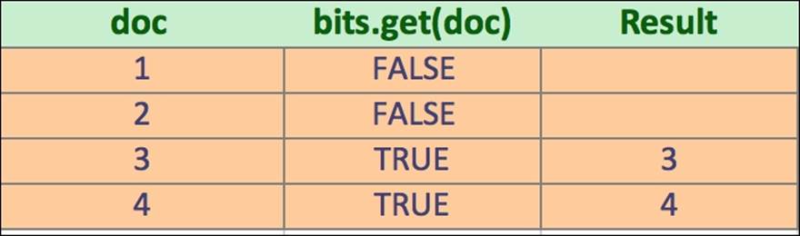
Lucene (and Elasticsearch) have various implementation of DocIdSet suitable for various cases. Each of the implementations differs when it comes to performance. However, choosing the correct implementation is the task of Lucene and Elasticsearch and we don't have to care about it, unless we extend the functionality of them.
Note
Please remember that not all filters use the Bits structure. The filters that don't do that are numeric range filters, script ones, and the whole group of geographical filters. Instead, those filters put data into the field data cache and iterate over documents filtering as they operate on a document. This means that the next filter in the chain will only get documents allowed by the previous filters. Because of this, those filters allow optimizations, such as putting the heaviest filters on the end of the filters, execution chain.
Bool or and/or/not filters
We talked about filters in Elasticsearch Server Second Edition, but we wanted to remind you about one thing. You should remember that and, or, and not filters don't use Bits, while the bool filter does. Because of that you should use the bool filter when possible. Theand, or, and not filters should be used for scripts, geographical filtering, and numeric range filters. Also, remember that if you nest any filter that is not using Bits inside the and, or, or not filter, Bits won't be used.
Basically, you should use the and, or, and not filters when you combine filters that are not using Bits with other filters. And if all your filters use Bits, then use the bool filter to combine them.
Performance considerations
In general, filters are fast. There are multiple reasons for this—first of all, the parts of the query handled by filters don't need to have a score calculated. As we have already said, scoring is strongly connected to a given query and the set of indexed documents.
Note
There is one thing when it comes to filtering. With the release of Elasticsearch 1.4.0, the bitsets used for nested queries execution are loaded eagerly by default. This is done to allow faster nested queries execution, but can lead to memory problems. To disable this behavior we can set the index.load_fixed_bitset_filters_eagerly to false. The size of memory used for fixed bitsets can be checked by using the curl -XGET 'localhost:9200/_cluster/stats?human&pretty' command and looking at thefixed_bit_set_memory_in_bytes property in the response.
When using a filter, the result of the filter does not depend on the query, so the result of the filter can be easily cached and used in the subsequent queries. What's more, the filter cache is stored as per Lucene segment, which means that the cache doesn't have to be rebuilt with every commit, but only on segment creation and segment merge.
Note
Of course, as with everything, there are also downsides of using filters. Not all filters can be cached. Think about filters that depend on the current time, caching them wouldn't make much sense. Sometimes caching is not worth it because of too many unique values that can be used and poor cache hit ratio, an example of this can be filters based on geographical location.
Post filtering and filtered query
If someone would say that the filter will be quicker comparing to the same query, it wouldn't be true. Filters have fewer things to care about and can be reused between queries, but Lucene is already highly optimized and the queries are very fast, even considering that scoring has to be performed. Of course, for a large number of results, filter will be faster, but there is always something we didn't tell you yet. Sometimes, when using post_filter, the query sent to Elasticsearch won't be as fast and efficient as we would want it to be. Let's assume that we have the following query:
curl -XGET 'http://127.0.0.1:9200/library/_search?pretty' -d '{
"query": {
"terms": {
"title": [ "crime", "punishment", "complete", "front" ]
}
},
"post_filter" : {
"term": {
"available": {
"value": true,
"_cache": true
}
}
}
}'
The following figure shows what is going on during query execution:
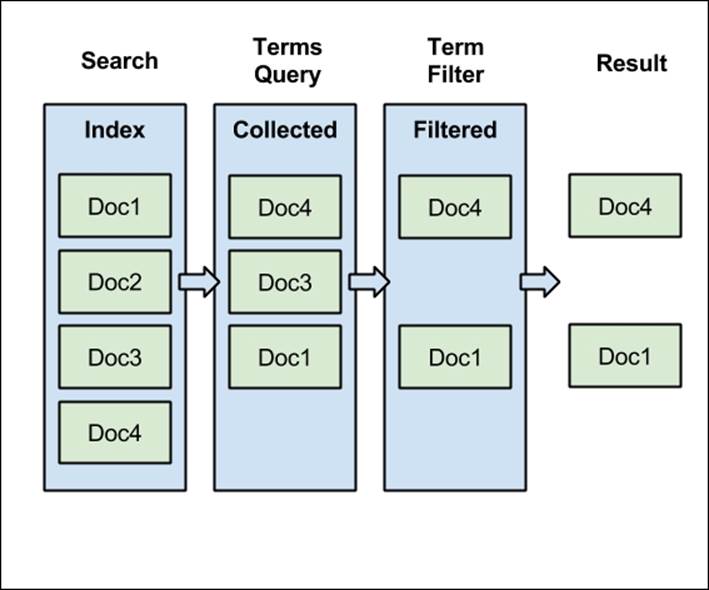
Of course, filtering matters for higher amounts of data, but for the purpose of this example, we've used our data. In the preceding figure, our index contains four documents. Our example terms query matches three documents: Doc1, Doc3, and Doc4. Each of them is scored and ordered on the basis of the calculated score. After that, our post_filter starts its work. From all of our documents in the whole index, it passes only two of them—Doc1 and Doc4. As you can see from the three documents passed to the filter, only two of them were returned as the search result. So why are we bothering about calculating the score for the Doc3? In this case, we lost some CPU cycles for scoring a document that are not valid in terms of query. For a large number of documents returned, this can become a performance problem.
Note
Please note that in the example we've used the term filter, which was cached by default until Elasticsearch 1.5. That behavior changed starting with Elasticsearch 1.5 (see https://github.com/elasticsearch/elasticsearch/pull/7583). Because of that, we decided to use the term filter in the example, but with forced caching.
Let's modify our query and let's filter the documents before the Scorer calculates the score for each document. The query that does that looks as follows:
curl -XGET 'http://127.0.0.1:9200/library/_search?pretty' -d '{
"query": {
"filtered": {
"query": {
"terms": {
"title": [ "crime", "punishment", "complete", "front" ]
}
},
"filter": {
"term": {
"available": {
"value": true,
"_cache": true
}
}
}
}
}
}'
In the preceding example, we have used the filtered query. The results returned by the preceding query will be exactly the same, but the execution of the query will be a little bit different, especially when it comes to filtering. Let's look at the following figure showing the logical execution of the query:
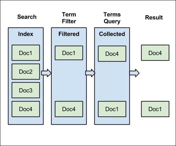
Now the initial work is done by the term filter. If it was already used, it will be loaded from the cache, and the whole document set will be narrowed down to only two documents. Finally, those documents are scored, but now the scoring mechanism has less work to do. Of course, in the example, our query matches the documents returned by the filter, but this is not always true.
Technically, our filter is wrapped by query, and internally Lucene library collects results only from documents that meet the enclosed filter criteria. And, of course, only the documents matching the filter are forwarded to the main query. Thanks to filter, the scoring process has fewer documents to look at.
Choosing the right filtering method
If you read the preceding explanations, you may think that you should always use the filtered query and run away from post filtering. Such statement will be true for most use cases, but there are exceptions to this rule. The rule of thumb says that the most expensive operations should be moved to the end of query processing. If the filter is fast, cheap, and easily cacheable, then the situation is simple—use filtered query. On the other hand, if the filter is slow, CPU-intensive, and hard to cache (i.e., because of too many distinct values), use post filtering or try to optimize the filter by simplifying it and making it more cache friendly, for example by reducing the resolution in case of time-based filters.
Choosing the right query for the job
In our Elasticsearch Server Second Edition, we described the full query language, the so-called Query DSL provided by Elasticsearch. A JSON structured query language that allows us to virtually build as complex queries as we can imagine. What we didn't talk about is when the queries can be used and when they should be used. For a person who doesn't have much prior experience with a full text search engine, the number of queries exposed by Elasticsearch can be overwhelming and very confusing. Because of that, we decided to extend what we wrote in the second edition of our first Elasticsearch book and show you, the reader, what you can do with Elasticsearch.
We decided to divide the following section into two distinct parts. The first part will try to categorize the queries and tell you what to expect from a query in that category. The second part will show you an example usage of queries from each group and will discuss the differences. Please take into consideration that the following section is not a full reference for the Elasticsearch Query DSL, for such reference please see Elasticsearch Server Second Edition from Packt Publishing or official Elasticsearch documentation available at http://www.elasticsearch.org/guide/en/elasticsearch/reference/current/query-dsl.html.
Query categorization
Of course, categorizing queries is a hard task and we don't say that the following list of categories is the only correct one. We would even say that if you would ask other Elasticsearch users, they would provide their own categories or say that each query can be assigned to more than a single category. What's funny—they would be right. We also think that there is no single way of categorizing the queries; however, in our opinion, each Elasticsearch query can be assigned to one (or more) of the following categories:
· Basic queries: Category that groups queries allowing searching for a part of the index, either in an analyzed or a non-analysed manner. The key point in this category is that you can nest queries inside a basic query. An example of a basic query is the termquery.
· Compound queries: Category grouping queries that allow us to combine multiple queries or filters inside them, for example a bool or dismax queries.
· Not analyzed queries: Category for queries that don't analyze the input and send it as is to Lucene index. An example of such query is the term query.
· Full text search queries: Quite a large group of queries supporting full text searching, analysing their content, and possibly providing Lucene query syntax. An example of such query is the match query.
· Pattern queries: Group of queries providing support for various wildcards in queries. For example, a prefix query can be assigned to this particular group.
· Similarity supporting queries: Group of queries sharing a common feature—support for match of similar words of documents. An example of such query is the fuzzy_like_this or the more_like_this query.
· Score altering queries: Very important group of queries, especially when combined with full text searching. This group includes queries that allow us to modify the score calculation during query execution. An example query that we can assign to this group is the function_score query, which we will talk about in detail in Chapter 3, Not Only Full Text Search.
· Position aware queries: Queries that allow us to use term position information stored in the index. A very good example of such queries is the span_term query.
· Structure aware queries: Group of queries that can work on structured data such as the parent–child documents. An example query from this group is the nested one.
Of course, we didn't talk about the filters at all, but you can use the same logic as for queries, so let's put the filters aside for now. Before going into examples for each type of query, let's briefly describe the purpose of each of the query category.
Basic queries
Queries that are not able to group any other queries, but instead they are used for searching the index only. Queries in this group are usually used as parts of the more complex queries or as single queries sent against Elasticsearch. You can think about those queries as bricks for building structures—more complex queries. For example, when you need to match a certain phrase in a document without any additional requirements, you should look at the basic queries—in such a case, the match query will be a good opportunity for this requirement and it doesn't need to be added by any other query.
Some examples of the queries from basic category are as follows:
· Match: A Query (actually multiple types of queries) used when you need a full text search query that will analyze the provided input. Usually, it is used when you need analysis of the provided text, but you don't need full Lucene syntax support. Because this query doesn't go through the query parsing process, it has a low chance of resulting in a parsing error, and because of this it is a good candidate for handling text entered by the user.
· match_all: A simple query matching all documents useful for situations when we need all the whole index contents returned for aggregations.
· term: A simple, not analyzed query that allows us to search for an exact word. An example use case for the term query is searching against non-analyzed fields, like ones storing tags in our example data. The term query is also used commonly combined with filtering, for example filtering on category field from our example data.
The queries from the complex category are: match, multi_match, common, fuzzy_like_this, fuzzy_like_this_field, geoshape, ids, match_all, query_string, simple_query_string, range, prefix, regexp, span_term, term, terms, wildcard.
Compound queries
Compound queries are the ones that we can use for grouping other queries together and this is their only purpose. If the simple queries were bricks for building houses, the complex queries are joints for those bricks. Because we can create a virtually indefinite level of nesting of the compound queries, we are able to produce very complex queries, and the only thing that limits us is performance.
Some examples of the compound queries and their usage are as follows:
· bool: One of the most common compound query that is able to group multiple queries with Boolean logical operator that allows us to control which part of the query must match, which can and which should not match. For example, if we would like to find and group together queries matching different criteria, then the bool query is a good candidate. The bool query should also be used when we want the score of the documents to be a sum of all the scores calculated by the partial queries.
· dis_max: A very useful query when we want the score of the document to be mostly associated with the highest boosting partial query, not the sum of all the partial queries (like in the bool query). The dis_max query generates the union of the documents returned by all the subqueries and scores the documents by the simple equation max (score of the matching clauses) + tie_breaker * (sum of scores of all the other clauses that are not max scoring ones). If you want the max scoring subquery to dominate the score of your documents, then the dis_max query is the way to go.
The queries from that category are: bool, boosting, constant_score, dis_max, filtered, function_score, has_child, has_parent, indices, nested, span_first, span_multi, span_first, span_multi, span_near, span_not, span_or, span_term, top_children.
Not analyzed queries
These are queries that are not analyzed and instead the text we provide to them is sent directly to Lucene index. This means that we either need to be aware exactly how the analysis process is done and provide a proper term, or we need to run the searches against the non-analyzed fields. If you plan to use Elasticsearch as NoSQL store this is probably the group of queries you'll be using, they search for the exact terms without analysing them, i.e., with language analyzers.
The following examples should help you understand the purpose of not analyzed queries:
· term: When talking about the not analyzed queries, the term query will be the one most commonly used. It provides us with the ability to match documents having a certain value in a field. For example, if we would like to match documents with a certain tag (tags field in our example data), we would use the term query.
· Prefix: Another type of query that is not analyzed. The prefix query is commonly used for autocomplete functionality, where the user provides a text and we need to find all the documents having terms that start with the given text. It is good to remember that even though the prefix query is not analyzed, it is rewritten by Elasticsearch so that its execution is fast.
The queries from that category are: common, ids, prefix, span_term, term, terms, wildcard.
Full text search queries
A group that can be used when you are building your Google-like search interface. Those queries analyze the provided input using the information from the mappings, support Lucene query syntax, support scoring capabilities, and so on. In general, if some part of the query you are sending comes from a user entering some text, you'll want to use one of the full text search queries such as the query_string, match or simple_query_string queries.
A Simple example of the full text search queries use case can be as follows:
· simple_query_string: A query built on top of Lucene SimpleQueryParser (http://lucene.apache.org/core/4_9_0/queryparser/org/apache/lucene/queryparser/simple/SimpleQueryParser.html) that was designed to parse human readable queries. In general, if you want your queries not to fail when a query parsing error occurs and instead figure out what the user wanted to achieve, this is a good query to consider.
The queries from that category are: match, multi_match, query_string, simple_query_string.
Pattern queries
Elasticsearch provides us with a few queries that can handle wildcards directly or indirectly, for example the wildcard query and the prefix query. In addition to that, we are allowed to use the regexp query that can find documents that have terms matching given patterns.
We've already discussed an example using the prefix query, so let's focus a bit on the regexp query. If you want a query that will find documents having terms matching a certain pattern, then the regexp query is probably the only solution for you. For example, if you store logs in your Elasticsearch indices and you would like to find all the logs that have terms starting with the err prefix, then having any number of characters and ending with memory, the regexp query will be the one to look for. However, remember that all the wildcard queries that have expressions matching large number of terms will be expensive when it comes to performance.
The queries from that category are: prefix, regexp, wildcard.
Similarity supporting queries
We like to think that the similarity supporting queries is a family of queries that allow us to search for similar terms or documents to the one we passed to the query. For example, if we would like to find documents that have terms similar to crimea term, we could run a fuzzy query. Another use case for this group of queries is providing us with "did you mean" like functionality. If we would like to find documents that have titles similar to the input we've provided, we would use the more_like_this query. In general, you would use a query from this group whenever you need to find documents having terms or fields similar to the provided input.
The queries from that category are: fuzzy_like_this, fuzzy_like_this_field, fuzzy, more_like_this, more_like_this_field.
Score altering queries
A group of queries used for improving search precision and relevance. They allow us to modify the score of the returned documents by providing not only a custom boost factor, but also some additional logic. A very good example of a query from this group is thefunction_score query that provides us with a possibility of using functions, which result in document score modification based on mathematical equations. For example, if you would like the documents that are closer to a given geographical point to be scored higher, then using the function_score query provides you with such a possibility.
The queries from that category are: boosting, constant_score, function_score, indices.
Position aware queries
These are a family of queries that allow us to match not only certain terms but also the information about the terms' positions. The most significant queries from this group are all the span queries in Elasticsearch. We can also say that the match_phrase query can be assigned to this group as it also looks at the position of the indexed terms, at least to some extent. If you want to find groups of words that are a certain distance in the index from other words, like "find me the documents that have mastering and Elasticsearch terms near each other and are followed by second and edition terms no further than three positions away," then span queries is the way to go. However, you should remember that span queries will be removed in future versions of Lucene library and thus from Elasticsearch as well. This is because those queries are resource-intensive and require vast amount of CPU to be properly handled.
The queries from that category are: match_phrase, span_first, span_multi, span_near, span_not, span_or, span_term.
Structure aware queries
The last group of queries is the structure aware queries. The queries that can be assigned to this group are as follows:
· nested
· has_child
· has_parent
· top_children
Basically, all the queries that allow us to search inside structured documents and don't require us to flatten the data can be classified as the structure aware queries. If you are looking for a query that will allow you to search inside the children document, nested documents, or for children having certain parents, then you need to use one of the queries that are mentioned in the preceding terms. If you want to handle relationships in the data, this is the group of queries you should look for; however, remember that although Elasticsearch can handle relations, it is still not a relational database.
The use cases
As we already know which groups of queries can be responsible for which tasks and what can we achieve using queries from each group, let's have a look at example use cases for each of the groups so that we can have a better view of what the queries are useful for. Please note that this is not a full and comprehensive guide to all the queries available in Elasticsearch, but instead a simple example of what can be achieved.
Example data
For the purpose of the examples in this section, we've indexed two additional documents to our library index.
First, we need to alter the index structure a bit so that it contains nested documents (we will need them for some queries). To do that, we will run the following command:
curl -XPUT 'http://localhost:9200/library/_mapping/book' -d '{
"book" : {
"properties" : {
"review" : {
"type" : "nested",
"properties": {
"nickname" : { "type" : "string" },
"text" : { "type" : "string" },
"stars" : { "type" : "integer" }
}
}
}
}
}'
The commands used for indexing two additional documents are as follows:
curl -XPOST 'localhost:9200/library/book/5' -d '{
"title" : "The Sorrows of Young Werther",
"author" : "Johann Wolfgang von Goethe",
"available" : true,
"characters" : ["Werther",
"Lotte","Albert",
" Fräulein von B"],
"copies" : 1,
"otitle" : "Die Leiden des jungen Werthers",
"section" : 4,
"tags" : ["novel", "classics"],
"year" : 1774,
"review" : [{"nickname" : "Anna","text" : "Could be good, but not my style","stars" : 3}]
}'
curl -XPOST 'localhost:9200/library/book/6' -d '{
"title" : "The Peasants",
"author" : "Władysław Reymont",
"available" : true,
"characters" : ["Maciej Boryna","Jankiel","Jagna Paczesiówna", "Antek Boryna"],
"copies" : 4,
"otitle" : "Chłopi",
"section" : 4,
"tags" : ["novel", "polish", "classics"],
"year" : 1904,
"review" : [{"nickname" : "anonymous","text" : "awsome book","stars" : 5},{"nickname" : "Jane","text" : "Great book, but too long","stars" : 4},{"nickname" : "Rick","text" : "Why bother, when you can find it on the internet","stars" : 3}]
}'
Basic queries use cases
Let's look at simple use cases for the basic queries group.
Searching for values in range
One of the simplest queries that can be run is a query matching documents in a given range of values. Usually, such queries are a part of a larger query or a filter. For example, a query that would return books with the number of copies from 1 to 3 inclusive would look as follows:
curl -XGET 'localhost:9200/library/_search?pretty' -d '{
"query" : {
"range" : {
"copies" : {
"gte" : 1,
"lte" : 3
}
}
}
}'
Simplified query for multiple terms
Imagine a situation where your users can show a number of tags the books returned by what the query should contain. The thing is that we require only 75 percent of the provided tags to be matched if the number of tags provided by the user is higher than three, and all the provided tags to be matched if the number of tags is three or less. We could run a bool query to allow that, but Elasticsearch provides us with the terms query that we can use to achieve the same requirement. The command that sends such query looks as follows:
curl -XGET 'localhost:9200/library/_search?pretty' -d '{
"query" : {
"terms" : {
"tags" : [ "novel", "polish", "classics", "criminal", "new" ],
"minimum_should_match" : "3<75%"
}
}
}'
Compound queries use cases
Let's now see how we can use compound queries to group other queries together.
Boosting some of the matched documents
One of the simplest examples is using the bool query to boost some documents by including not mandatory query part that is used for boosting. For example, if we would like to find all the books that have at least a single copy and boost the ones that are published after 1950, we could use the following query:
curl -XGET 'localhost:9200/library/_search?pretty' -d '{
"query" : {
"bool" : {
"must" : [
{
"range" : {
"copies" : {
"gte" : 1
}
}
}
],
"should" : [
{
"range" : {
"year" : {
"gt" : 1950
}
}
}
]
}
}
}'
Ignoring lower scoring partial queries
The dis_max query, as we have already covered, allows us to control how influential the lower scoring partial queries are. For example, if we only want to assign the score of the highest scoring partial query for the documents matching crime punishment in the titlefield or raskolnikov in the characters field, we would run the following query:
curl -XGET 'localhost:9200/library/_search?pretty' -d '{
"fields" : [ "_id", "_score" ],
"query" : {
"dis_max" : {
"tie_breaker" : 0.0,
"queries" : [
{
"match" : {
"title" : "crime punishment"
}
},
{
"match" : {
"characters" : "raskolnikov"
}
}
]
}
}
}'
The result for the preceding query should look as follows:
{
"took" : 3,
"timed_out" : false,
"_shards" : {
"total" : 5,
"successful" : 5,
"failed" : 0
},
"hits" : {
"total" : 1,
"max_score" : 0.2169777,
"hits" : [ {
"_index" : "library",
"_type" : "book",
"_id" : "4",
"_score" : 0.2169777,
"fields" : {
"_id" : "4"
}
} ]
}
}
Now let's see the score of the partial queries alone. To do that we will run the partial queries using the following commands:
curl -XGET 'localhost:9200/library/_search?pretty' -d '{
"fields" : [ "_id", "_score" ],
"query" : {
"match" : {
"title" : "crime punishment"
}
}
}'
The response for the preceding query is as follows:
{
"took" : 2,
"timed_out" : false,
"_shards" : {
"total" : 5,
"successful" : 5,
"failed" : 0
},
"hits" : {
"total" : 1,
"max_score" : 0.2169777,
"hits" : [ {
"_index" : "library",
"_type" : "book",
"_id" : "4",
"_score" : 0.2169777,
"fields" : {
"_id" : "4"
}
} ]
}
}
And the next command is as follows:
curl -XGET 'localhost:9200/library/_search?pretty' -d '{
"fields" : [ "_id", "_score" ],
"query" : {
"match" : {
"characters" : "raskolnikov"
}
}
}'
And the response is as follows:
{
"took" : 1,
"timed_out" : false,
"_shards" : {
"total" : 5,
"successful" : 5,
"failed" : 0
},
"hits" : {
"total" : 1,
"max_score" : 0.15342641,
"hits" : [ {
"_index" : "library",
"_type" : "book",
"_id" : "4",
"_score" : 0.15342641,
"fields" : {
"_id" : "4"
}
} ]
}
}
As you can see, the score of the document returned by our dis_max query is equal to the score of the highest scoring partial query (the first partial query). That is because we've set the tie_breaker property to 0.0.
Not analyzed queries use cases
Let's look at two example use cases for queries that are not processed by any of the defined analyzers.
Limiting results to given tags
One of the simplest examples of the not analyzed query is the term query provided by Elasticsearch. You'll probably very rarely use the term query alone; however, it may be commonly used in compound queries. For example, let's assume that we would like to search for all the books with the novel value in the tags field. To do that, we would run the following command:
curl -XGET 'localhost:9200/library/_search?pretty' -d '{
"query" : {
"term" : {
"tags" : "novel"
}
}
}'
Efficient query time stopwords handling
Elasticsearch provides the common terms query, which allows us to handle query time stopwords in an efficient way. It divides the query terms into two groups—more important terms and less important terms. The more important terms are the ones that have a lower frequency; the less important terms are the opposite. Elasticsearch first executes the query with important terms and calculates the score for those documents. Then, a second query with the less important terms is executed, but the score is not calculated and thus the query is faster.
For example, the following two queries should be similar in terms of results, but not in terms of score computation. Please also note that to see the differences in scoring we would have to use a larger data sample and not use index time stopwords:
curl -XGET 'localhost:9200/library/_search?pretty' -d '{
"query" : {
"common" : {
"title" : {
"query" : "the western front",
"cutoff_frequency" : 0.1,
"low_freq_operator": "and"
}
}
}
}'
And the second query would be as follows:
curl -XGET 'localhost:9200/library/_search?pretty' -d '{
"query" : {
"bool" : {
"must" : [
{
"term" : { "title" : "western" }
},
{
"term" : { "title" : "front" }
}
],
"should" : [
{
"term" : { "title" : "the" }
}
]
}
}
}'
Full text search queries use cases
Full text search is a broad topic and so are the use cases for the full text queries. However, let's look at two simple examples of queries from that group.
Using Lucene query syntax in queries
Sometimes, it is good to be able to use Lucene query syntax as it is. We talked about this syntax in the Lucene query language section in Chapter 1, Introduction to Elasticsearch. For example, if we would like to find books having sorrows and young terms in their title, von goethe phrase in the author field and not having more than five copies we could run the following query:
curl -XGET 'localhost:9200/library/_search?pretty' -d '{
"query" : {
"query_string" : {
"query" : "+title:sorrows +title:young +author:\"von goethe\" - copies:{5 TO *]"
}
}
}'
As you can see, we've used the Lucene query syntax to pass all the matching requirements and we've let query parser construct the appropriate query.
Handling user queries without errors
Sometimes, queries coming from users can contain errors. For example, let's look at the following query:
curl -XGET 'localhost:9200/library/_search?pretty' -d '{
"query" : {
"query_string" : {
"query" : "+sorrows +young \"",
"default_field" : "title"
}
}
}'
The response would contain the following:
"error" : "SearchPhaseExecutionException[Failed to execute phase [query]
This means that the query was not properly constructed and parse error happened. That's why the simple_query_string query was introduced. It uses a query parser that tries to handle user mistakes and tries to guess how the query should look. Our query using that parser would look as follows:
curl -XGET 'localhost:9200/library/_search?pretty' -d '{
"query" : {
"simple_query_string" : {
"query" : "+sorrows +young \"",
"fields" : [ "title" ]
}
}
}'
If you run the preceding query, you would see that the proper document has been returned by Elasticsearch, even though the query is not properly constructed.
Pattern queries use cases
There are multiple use cases for the wildcard queries; however, we wanted to show you the following two.
Autocomplete using prefixes
A very common use case provides autocomplete functionality on the indexed data. As we know, the prefix query is not analyzed and works on the basis of terms indexed in the field. So the actual functionality depends on what tokens are produced during indexing. For example, let's assume that we would like to provide autocomplete functionality on any token in the title field and the user provided wes prefix. A query that would match such a requirement looks as follows:
curl -XGET 'localhost:9200/library/_search?pretty' -d '{
"query" : {
"prefix" : {
"title" : "wes"
}
}
}'
Pattern matching
If we need to match a certain pattern and our analysis chain is not producing tokens that allow us to do so, we can turn into the regexp query. One should remember, though, that this kind of query can be expensive during execution and thus should be avoided. Of course, this is not always possible. One thing to remember is that the performance of the regexp query depends on the chosen regular expression. If you choose a regular expression that will be rewritten into a high number of terms, then performance will suffer.
Let's now see the example usage of the regexp query. Let's assume that we would like to find documents that have a term starting with wat, then followed by two characters and ending with the n character, and those terms should be in the characters field. To match this requirement, we could use a regexp query like the one used in the following command:
curl -XGET 'localhost:9200/library/_search?pretty' -d '{
"query" : {
"regexp" : {
"characters" : "wat..n"
}
}
}'
Similarity supporting queries use cases
Let's look at a couple of simple use cases about how we can find similar documents and terms.
Finding terms similar to a given one
A very simple example is using the fuzzy query to find documents having a term similar to a given one. For example, if we would like to find all the documents having a value similar to crimea, we could run the following query:
curl -XGET 'localhost:9200/library/_search?pretty' -d '{
"query" : {
"fuzzy" : {
"title" : {
"value" : "crimea",
"fuzziness" : 3,
"max_expansions" : 50
}
}
}
}'
Finding documents with similar field values
Another example of similarity queries is a use case when we want to find all the documents having field values similar to what we provided in a query. For example, if we would like to find books having a title similar to the western front battles name, we could run the following query:
curl -XGET 'localhost:9200/library/_search?pretty' -d '{
"query" : {
"fuzzy_like_this_field" : {
"title" : {
"like_text" : "western front battles",
"max_query_terms" : 5
}
}
}
}'
The result of the preceding query would be as follows:
{
"took" : 10,
"timed_out" : false,
"_shards" : {
"total" : 5,
"successful" : 5,
"failed" : 0
},
"hits" : {
"total" : 2,
"max_score" : 1.0162667,
"hits" : [ {
"_index" : "library",
"_type" : "book",
"_id" : "1",
"_score" : 1.0162667,
"_source":{ "title": "All Quiet on the Western Front","otitle": "Im Westen nichts Neues","author": "Erich Maria Remarque","year": 1929,"characters": ["Paul B├Ąumer", "Albert Kropp", "Haie Westhus", "Fredrich M├╝ller", "Stanislaus Katczinsky", "Tjaden"],"tags": ["novel"],"copies": 1,
"available": true, "section" : 3}
}, {
"_index" : "library",
"_type" : "book",
"_id" : "5",
"_score" : 0.4375,
"_source":{"title" : "The Sorrows of Young Werther","author" : "Johann Wolfgang von Goethe","available" : true,"characters" : ["Werther","Lotte","Albert","Fraulein von B"],"copies" : 1, "otitle" : "Die Leiden des jungen Werthers","section" : 4,"tags" : ["novel", "classics"],"year" : 1774,"review" : [{"nickname" : "Anna","text" : "Could be good, but not my style","stars" : 3}]}
} ]
}
}
As you can see, sometimes the results are not as obvious as we would expect (look at the second book title). This is because of what Elasticsearch thinks is similar to each other. In the case of the preceding query, Elasticsearch will take all the terms, run a fuzzy search on them, and choose a number of best differentiating terms for documents matching.
Score altering queries use cases
When it comes to relevancy, Elasticsearch provides us with a few queries that we can use to alter the score as per our need. Of course, in addition to this, most queries allow us to provide boost, which gives us even more control. Let's now look at two example use cases of score altering queries.
Favoring newer books
Let's assume that we would like to favor books that are newer, so that a book from the year 1986 is higher in the results list than a book from 1870. The query that would match that requirement looks as follows:
curl -XGET 'localhost:9200/library/_search?pretty' -d '{
"query" : {
"function_score" : {
"query" : {
"match_all" : {}
},
"score_mode" : "multiply",
"functions" : [
{
"gauss" : {
"year" : {
"origin" : 2014,
"scale" : 2014,
"offset" : 0,
"decay": 0.5
}
}
}
]
}
}
}'
We will discuss the function_score query in Chapter 3, Not Only Full Text Search. For now, if you look at the results returned by the preceding query, you can see that the newer the book, the higher in the results it will be.
Decreasing importance of books with certain value
Sometimes, it is good to be able to decrease the importance of certain documents, while still showing them in the results list. For example, we may want to show all books, but put the ones that are not available on the bottom of the results list by lowering their score. We don't want sorting on availability because sometimes use may know what he or she is looking for and the score of a full text search query should be also important. However, if our use case is that we want the books that are not available on the bottom of the results list, we could use the following command to get them:
curl -XGET 'localhost:9200/library/_search?pretty' -d '{
"query" : {
"boosting" : {
"positive" : {
"match_all" : {}
},
"negative" : {
"term" : {
"available" : false
}
},
"negative_boost" : 0.2
}
}
}'
Pattern queries use cases
Not very commonly used because of how resource hungry they are, pattern aware queries allow us to match documents having phrases and terms in the right order. Let's look at some examples.
Matching phrases
The simplest position aware query possible and the most performing one from the queries assigned in this group. For example, a query that would only match document leiden des jungen phrase in the otitle field would look as follows:
curl -XGET 'localhost:9200/library/_search?pretty' -d '{
"query" : {
"match_phrase" : {
"otitle" : "leiden des jungen"
}
}
}'
Spans, spans everywhere
Of course, the phrase query is very simple when it comes to position handling. What if we would like to run a query to find documents that have des jungen phrase not more than two positions after the die term and just before the werthers term? This can be done with span queries, and the following command shows how such a query could look:
curl -XGET 'localhost:9200/library/_search?pretty' -d '{
"query" : {
"span_near" : {
"clauses" : [
{
"span_near" : {
"clauses" : [
{
"span_term" : {
"otitle" : "die"
}
},
{
"span_near" : {
"clauses" : [
{
"span_term" : {
"otitle" : "des"
}
},
{
"span_term" : {
"otitle" : "jungen"
}
}
],
"slop" : 0,
"in_order" : true
}
}
],
"slop" : 2,
"in_order" : false
}
},
{
"span_term" : {
"otitle" : "werthers"
}
}
],
"slop" : 0,
"in_order" : true
}
}
}'
Please note that span queries are not analyzed. We can see that by looking at the response of the Explain API. To see that response, we should run the same request body (our query) to the /library/book/5/_explain REST endpoint. The interesting part of the output looks as follows:
"description" : "weight(spanNear([spanNear([otitle:die, spanNear([otitle:des, otitle:jungen], 0, true)], 2, false), otitle:werthers], 0, true) in 1) [PerFieldSimilarity], result of:",
Structure aware queries use cases
When it comes to the nested documents or the parent–child relationship, structure aware queries are the ones that will be needed sooner or later. Let's look at the following two examples of where the structure query can be used.
Returning parent documents having a certain nested document
The first example will be a very simple one. Let's return all the books that have at least a single review that was given four stars or more. The query that does that looks as follows:
curl -XGET 'localhost:9200/library/_search?pretty' -d '{
"query" : {
"nested" : {
"path" : "review",
"query" : {
"range" : {
"stars" : {
"gte" : 4
}
}
}
}
}
}'
Affecting parent document score with the score of nested documents
Let's assume that we want to find all the available books that have reviews and let's sort them on the maximum number of stars given in the review. The query that would fill such a requirement looks as follows:
curl -XGET 'localhost:9200/library/_search?pretty' -d '{
"query" : {
"nested" : {
"path" : "review",
"score_mode" : "max",
"query" : {
"function_score" : {
"query" : { "match_all" : {} },
"score_mode" : "max",
"boost_mode" : "replace",
"field_value_factor" : {
"field" : "stars",
"factor" : 1,
"modifier" : "none"
}
}
}
}
}
}'
Summary
In this chapter, we've looked at how the default Apache Lucene scoring works and we've discussed the query rewrite process—how it is done and why is it needed. We've discussed how query templates work and how they can simplify your queries. We've also looked at different query filtering methods, how they differ in comparison to each other, and when they can be used. Finally, we've assigned queries to different groups, we've learned when which query group can be used, and we've seen some example queries for each of the groups.
In the next chapter, we'll step away from full text search and focus on other search functionalities. We will start by extending our knowledge about the rescore functionality and the ability to recalculate the score for top documents in the results. After that we will look at how to load significant terms and add documents grouping using aggregations. We will also compare parent–child relationships to the nested documents, we will use function queries and, finally, we will learn how to efficiently page documents.
All materials on the site are licensed Creative Commons Attribution-Sharealike 3.0 Unported CC BY-SA 3.0 & GNU Free Documentation License (GFDL)
If you are the copyright holder of any material contained on our site and intend to remove it, please contact our site administrator for approval.
© 2016-2026 All site design rights belong to S.Y.A.