Emerging Trends in Image Processing, Computer Vision, and Pattern Recognition, 1st Edition (2015)

Part II. Computer Vision and Recognition Systems

Chapter 27. Automatic classification of protein crystal images

Madhav Sigdel¹; Madhu S. Sigdel¹; İmren Dinç¹; Semih Dinç¹; Marc L. Pusey²; Ramazan S. Aygün^{1 1} DataMedia Research Lab, Computer Science Department, University of Alabama Huntsville, Huntsville, AL, USA
² iXpressGenes Inc., Huntsville, AL, USA

Abstract

This work introduces our method for automatic classification of crystallization trial images according to the types of protein crystals present in the images. The images are classified into four categories: needles, small crystals, large crystals, and other crystals. Because protein crystals are characterized by some geometric shapes, we focus on extracting geometric features from the images. Our image feature extraction includes extraction of blob features from multiple binary images, extraction of edge related features from Canny edge image, and extraction of line features using Hough line transform. For the decision model, we propose applying random forest classifier. We performed our experiments on 212 expert labeled images with different classifiers and tested our results using 10-fold cross validation. The proposed classification technique produces a reasonable performance for protein crystallization image classification. The overall accuracy using random forest is 78%.

Keywords

Protein crystallization

Crystal classification

Blob features

Edge features

Acknowledgment

This research was supported by National Institutes of Health (GM090453) grant.

1 Introduction

Protein crystallization is the process for formation of protein crystals. Success of protein crystallization is dependent on several factors such as protein concentration, type of precipitant, crystallization methods, etc. Therefore, thousands of crystallization trials with different crystallization conditions are required for successful crystallization [1]. High throughput systems have been developed in recent years trying to identify the best conditions to crystallize proteins [1]. Imaging techniques are used to monitor the progress of crystallization. The crystallization trials are scanned periodically to determine the state change or the possibility of forming crystals. With a large number of images being captured, it is necessary to have a reliable classification system to distinguish the crystallization states each image belongs to. The main goal is to discard the unsuccessful trials, identify the successful trials, and possibly identify the trials which could be helpful. The main interest for crystallographers is the formation of large 3D crystals suitable for X-ray diffraction. Other crystal structures are also important as the crystallization conditions can be optimized to get better crystals. Therefore, it is necessary to have a reliable system that distinguishes between different types of crystals according to the shapes and sizes.

Many research studies have been done to distinguish crystallization trial images according to the presence or absence of crystals [2–6]. In our previous work [7], we presented classification of crystallization trials into three categories (non-crystals, likely-leads and crystals). Saitoh et al. [8] proposed crystallization into five categories (clear drop, creamy precipitate, granulated precipitate, amorphous state precipitate, and crystal) and Spraggon et al. [9] described classification into six categories (experimental mistake, clear drop, homogeneous precipitant, inhomogeneous precipitant, micro-crystals, and crystals). Likewise, Cumba et al. [10] classified crystallization trials into six basic categories (phase separation, precipitate, skin effect, crystal, junk, and unsure). In all these studies, the objective of the classification is to identify the different phases of crystallization. In other words, classification of protein crystal images according to the shapes and sizes of crystals has not been the main focus of the previous other work.

For feature extraction, a variety of image processing techniques have been proposed. Cumba et al. [2], Saitoh et al. [11], and Zhu et al. [12] used a combination of geometric and texture features as the input to their classifier. Saitoh et al. [8] used global texture features as well as features from local parts in the image and features from differential images. Cumba et al. [10] extracted several features such as basic statistics, energy, Euler numbers, Radon-Laplacian features, Sobel-edge features, micro-crystal features, and GLCM features to obtain a large feature vector. We presented classification using region features and edge features in Ref. [13]. Increasing the number of features may not necessarily improve the accuracy. Moreover, it may slow down the classification process. Therefore, finding a minimal set of useful image features for classification is important.

This work introduces our technique for automatic classification of trial images consisting of crystals. Our focus is on classifying crystallization trial images according to the types of protein crystals present in the images. Our previous study [13] attempted to classify trial images according to the types of crystals (needle crystals, small crystals, large crystals, other crystals). This work extends our earlier work [13] on crystallization trials classification. The main objective is to improve the classification accuracy with new additional image features and using an alternate classification technique. Our feature extraction includes extracting edge related features from Canny edge image, extracting blob related features from multiple binary images, and extracting line features using Hough transform. The images are classified into four categories: needles, small crystals, large crystals, and other crystals. For the decision model, we investigate random forest classifier in addition to decision tree classifier proposed in Ref. [13].

This chapter is arranged as follows. The following section describes the image categories for the classification problem considered in this paper. Section 3 provides the system overview. Section 4 describes the image processing and feature extraction steps used in our research. Experimental results and discussion are provided in Section 5. The last section concludes the chapter with future work.

2 Image Categories

The simplest classification of the crystallization trials distinguishes between the non-crystals (trial images not containing crystals) and crystals (images having crystals). In this study, we are interested in developing a system to classify different crystal types. We consider four image categories (needle crystals, small crystals, large crystals, and other crystals) for protein crystallization images consisting of crystals. Here description of each category is provided:

Needle crystals: Needle crystals have pointed edges and appear as needles. These crystals can appear alone or as a cluster in the images. The overlapping of multiple needle crystals on top of each other makes it difficult to get the correct crystal structure for these images. Figure 1 (a-c) show some sample crystal images under this category.

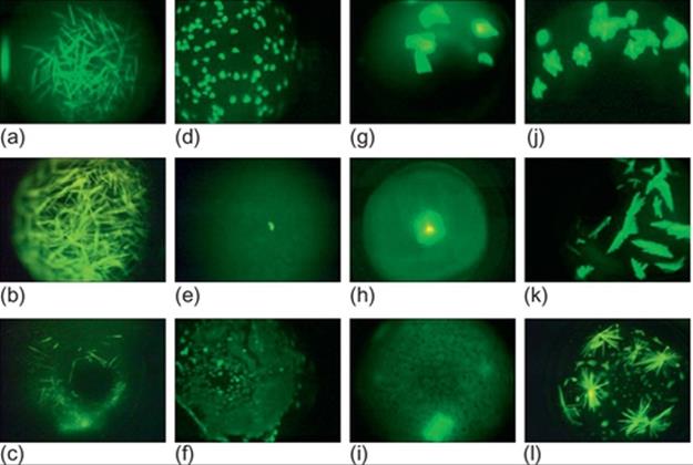
FIGURE 1 Sample protein crystallization images: (a-c) needles, (d-f) small crystals, (g-i) large crystals, and (j-l) other crystals.

Small crystals: This category contains small-sized crystals. These crystals can have two- or three-dimensional shapes. These crystals can also appear alone or as a cluster in the images. Because of their small size, it is difficult to visualize the geometric shapes expected in crystals. Besides, the crystals may be blurred because of focusing problems. Figure 1 (d-f) provide some sample images under this category.

Large crystals: This category includes images with large crystals with quadrangle (two- or three-) shapes. Depending on the orientation of protein crystals in the solution, more than one surface may be visible in some images. Figure 1 (g-i) show some sample images under this category.

Other crystals: The images in this category may be a combination of needles, plates, and other types of crystals. We can observe high intensity regions without proper geometric shapes expected in a crystal. This can be due to focusing problems. Some representative images are shown in Figure 1 (j-l).

3 System overview

The images of crystallization trials are collected using Crystal X2 software from iXpressGenes, Inc. The protein solutions are labeled with trace levels (<1%) of fluorescent dye. Green light is used as the flourescence excitation source while collecting the images [7].Figure 2 shows the system diagram of the crystallization trials to classify systems. We first down-sample the images by eightfold from 2560 × 1920 to 320 × 240 and crop 10 pixels at the borders from each side. This reduction enables feature extraction faster without losing necessary details for feature extraction. The downsampled image is input to the image binarization technique. Image segmentation is performed on the binary images, and region features are extracted. Likewise, Canny edge detection [14] is applied on the image. The Canny edge image is used to extract edge features, Harris corner [15] features and Hough [16] line features. Overall, we obtain a 45-dimensional feature vector for the classifier. All the image feature extraction and classifier routines are programmed in Matlab. The following section describes the image processing and feature extraction in more detail.

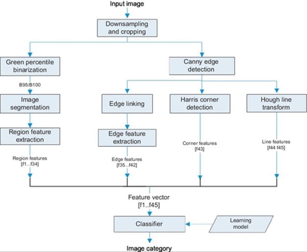
FIGURE 2 System diagram.

4 Image preprocessing and feature extraction

The distinguishing characteristics of protein crystals are the presence of straight lines and quadrangular shapes. Therefore, we focus on extracting geometric features of the objects (or regions) in the image. As in our previous work [13], we extract blob features from multiple binary images and edge features from Canny edge image. In addition to these features, we apply Hough line transform and extract line related features. Details of our proposed image processing and feature extraction technique is provided in the following section.

4.1 Green Percentile Image Binarization

Image binarization is a technique for separating foreground and background regions in an image. When green light is used as the excitation source for fluorescence based acquisition, the intensity of the green pixel component is observed to be higher than the red and blue components in the crystal regions [7]. We utilize this feature for our green percentile image binarization. Let τ_p be the threshold for green component intensity such that the number of pixels in the image with green component below τ_p constitute p% of the pixels. For example, if p = 90,τ₉₀ is the threshold of green intensity such that 90% of the green component pixels will be less than τ₉₀. Image is binarized using the value of τ_p and a minimum gray level intensity condition τ_min = 40. All pixels with gray level intensity greater than τ_min and having green pixel component greater than τ_p constitute the foreground region while the remaining pixels constitute the background region. As the value of p goes higher, the foreground (object) region in the binary image usually becomes smaller.

We generate binary images using green percentile thresholds for p=95 and p=99 and extract region features. Figure 3 shows some sample thresholded images using the two methods. From the original and binary images in Figure 3, we can observe that a single technique may not yield good results for all images. For the images in rows (i) and (ii), the binary images with p = 95 provide better representation of the crystal objects. However, for image at row (iii), the binary image obtained using p = 99 provides better representation of the crystals.

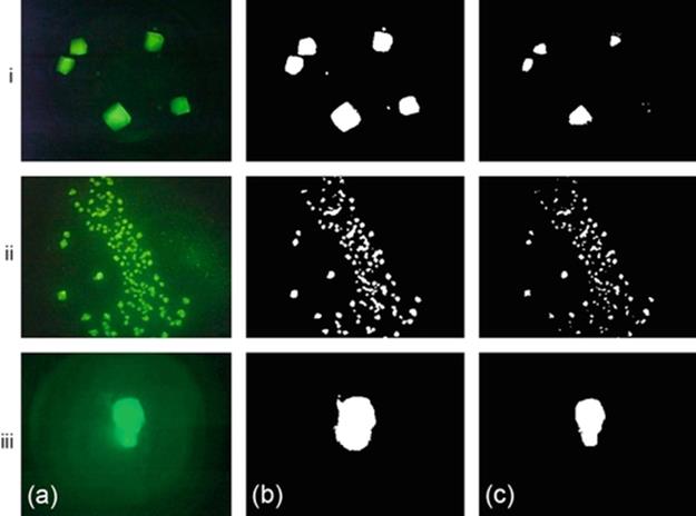
FIGURE 3 Image binarization on crystallization trial images: (a) original images, (b) Green percentile threshold (p = 95), and (c) Green percentile threshold (p = 99).

4.2 Region Features

After we generate the binary image, we apply connected component labeling to segment the regions (crystals). The binary image can be obtained from any of the thresholding methods. Let O be the set of the blobs in a binary image B, and B consists of n number of blobs. The blobs are ordered from the largest to the smallest such that area (O_i) ≥ area(O_i+1). Each blob O_i is enclosed by a minimum boundary rectangle (MBR) having width (w_i) and height (h_i). It should be noted that the blobs may not necessarily represent crystals in an image. For such cases, the blob features may not be particularly useful for the classifier. Table 1 provides a list of the region features. We extract five features (area, perimeter, filled area, convex area, and eccentricity) from the three largest blobs O₁, O₂, and O₃. If the number of blobs is less than 3, value 0 is assigned. We apply green percentile image binarization with p = 95 and p = 99. From each binary image, we extract 17 region features. Thus, at the end of this step, we obtain 34 features.

Table 1

Region Features

4.3 Edge Features

Canny edge detection algorithm [14] is one of the most reliable algorithms for edge detection. Our results show that for most cases, the shapes of crystals are kept intact in the resulting edge image. An edge image can contain many edges which may or may not be part of the crystals. To analyze the shape and other edge related features, we link the edges to form graphs. We used the MATLAB procedure by Kovesi [17] to perform this operation. The input to this step is a binary edge image. First, isolated pixels are removed from the input edge image. Next, the information of start and end points of the edges, endings and junctions are determined. From every end point, we track points along an edge until an end point or junction is encountered, and label the image pixels. The result of edge linking for the Canny edge image in Figure 4 (b) is shown in Figure 4 (c).

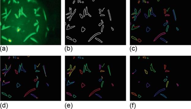
FIGURE 4 Edge detection and edge feature extraction: (a) original image, (b) Canny edge image, (c) edge linking, (d) line fitting, (e) edge cleaning, and (f) image with cyclic graphs or edges forming line normals.

Two points (vertices) connected by a line is an edge. Likewise, connected edges form a graph. Here, we use the terms edges and lines interchangeably. The number of graphs, the number of edges in a graph, the length of edges, angle between the edges, etc. are good features to distinguish different types of crystals. To extract these features, we do some preprocessing on the Canny edge image. Due to the problem with focusing, many edges can be formed. To reduce the number of edges and to link the edges together, line fitting is done. In this step, edges within certain deviation from a line are connected to form a single edge [17]. The result from line fitting is shown in Figure 4 (d). Here, the margin of three pixels is used as the maximum allowable deviation. From the figures, we can observe that after line fitting, the number of edges is reduced and the shapes resemble to the shapes of the crystals. Likewise, isolated edges and edges that are shorter than a minimum length are removed. The result from removing the unnecessary edges is shown in Figure 4 (e). At the end of edge linking procedure, we extract the eight edge related features listed in Table 2. The lengths of edges are calculated using Euclidean distance measure. Likewise, the angle between the edges is used to determine if the edges (lines) are normal to each other. We consider two lines to be normals if the angle θ between them lies between 60 and 120 (i.e., 60 ≤ θ ≤ 120).

Table 2

Edge Features

4.4 Corner Features

Corner points are considered as one of the uniquely recognizable features in an image. A corner is the intersection of two edges where the variation between two perpendicular directions is very high. Harris corner detection [15] exploits this idea and it basically measures the change in intensity of a pixel (x,y) for a displacement of a search window in all directions. We apply Harris corner detection and count the number of corners as the image feature.

4.5 Hough Line Features

Hough transform is a very popular technique in computer vision for detecting certain class of shapes by a voting procedure [16, 18]. We apply Hough line transform to detect lines in an image. Once the lines are detected, we extract the following two line features—number of Hough lines and the average length of line.

5 Experimental results

Our experimental dataset consists of 212 expert labeled images. The images are hand-labeled by an expert into four different categories: needles, small crystals, large crystals, and other crystals. The proportion of these classes are 24%, 20%, 35% and 21% respectively. For each image, we apply green percentile binarization with p = 95 and p = 99. From each binary image, we extract 17 region features. Likewise, we extract 8 edge related features, 1 Harris corner feature, and 2 Hough line features. Therefore, we extract a total of 2 × 17 + 8 + 1 + 2 = 45 features per image. On a Windows 7 Intel Core i7 CPU @2.4 GHz system with 12 GB memory, it takes around 232 s to extract features for 212 images. Thus the time for feature extraction is around 1.1 s per image.

We group the feature sets into three categories—region features, edge/corner/line features, and combined features. For the classification, we test using decision tree and random forest classifier. Table 3 shows the classification accuracy using the selected classifiers and feature sets. The values are computed as the average accuracy over 10 runs of 10-fold cross validation. Region features alone does not provide good accuracies. With edge-corner-line features only, we obtain 73% accuracy with decision tree and 75% accuracy with random forest. Combining the two features improves the overall accuracy.

Table 3

Classification Correctness Comparison

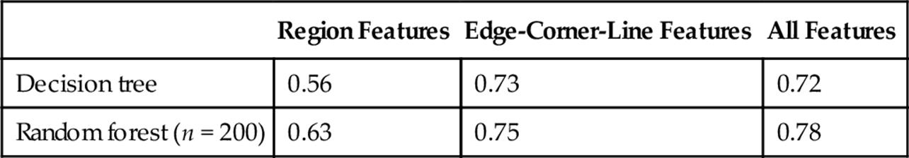
The best accuracy is obtained with random forest classifier and combined set of features. For this combination, we obtained accuracy in the range 75-80%. Table 4 shows a sample confusion matrix using 200 trees for the random forest. The overall accuracy is 78.3%. The sensitivity for large crystals is 88%.

Table 4

Confusion Matrix with Random Forest Classifier (Number of Trees = 200)

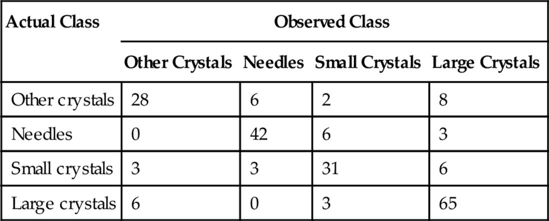
Among the four classes, we can observe that the system distinguishes the small crystals and needle crystals with high accuracy. Distinction between large crystals and other crystals is the most problematic. From our discussion with the expert, small and large crystals are the most important crystals in terms of their usability for the diffraction process. Therefore, it is critical not to misclassify the images in these categories into other two categories. From Table 1, we observe that our system misses 6 small crystals (3 images grouped as other crystals and 3 images grouped as needles). Likewise, our system classifies 6 large crystals as other crystals. In overall, our system misses 12 [3+3+6] critical images. Thus, the rate of miss of critical crystals of our system is around 6% [12/212]. This is a promising achievement for crystal sub-classification of crystal categories. The average accuracy over 10 runs of 10-fold cross validation is 78%.

As the number of trees for random forest classifier is increased, the accuracy is increased up to a certain extent. Figure 5 provides the performance comparison for accuracy and computation time for training and testing versus the number of trees. The best accuracy is obtained with number of trees sampled is 200. As the number of trees parameter for random forest increases, the computation time also increases. The computation time for training and testing time increases linearly with the number of trees.

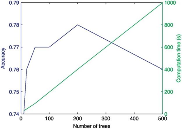
FIGURE 5 Performance comparison (accuracy and performance computation vs number of trees of random forest).

6 Conclusion and Future Work

This chapter describes our method for automatic classification of protein crystals in crystallization trial images. Our method focuses on extracting geometric features related to blobs, edges, and lines from the images. Using random forest classifier, we are able to achieve classification accuracy around 78% for a 4-class problem and this is a good classification performance.

This study focused on classifying a crystallization trial image according to the types of protein crystals present in the image. We only included images consisting crystals in our experiments. In the future, we would like to perform a two-level classification. First, we plan to classify the images as non-crystals, likely-crystals, and crystals. Next, we plan to classify the sub-categories. The current work will fall under the sub-classification of crystals.

We plan to improve the accuracy of the system further. The performance of our system depends on the accuracy of image binarization. In some images, the thresholded images do not capture the shapes of crystals correctly. Therefore, the features extracted from blobs may not necessarily represent crystals. Because of this, the features extracted from those blobs are not useful. To solve this problem, we plan to investigate different thresholding techniques. Our initial study shows that using the best thresholded image for feature extraction improves the classification performance.

References

[1] Pusey ML, Liu Z-J, Tempel W, Praissman J, Lin D, Wang B-C, et al. Life in the fast lane for protein crystallization and X-ray crystallography. Progr Biophys Molecul Biol. 2005;88(3):359–386.

[2] Cumbaa CA, Lauricella A, Fehrman N, Veatch C, Collins R, Luft J, et al. Automatic classification of sub-microlitre protein-crystallization trials in 1536-well plates. Acta Crystallograp D Biol Crystallograp. 2003;59(9):1619–1627.

[3] Cumbaa C, Jurisica I. Automatic classification and pattern discovery in high-throughput protein crystallization trials. J Struct Funct Genom. 2005;6(2–3):195–202.

[4] Berry IM, Dym O, Esnouf R, Harlos K, Meged R, Perrakis A, et al. Spine high-throughput crystallization, crystal imaging and recognition techniques: current state, performance analysis, new technologies and future aspects. Acta Crystallograph D Biol Crystallograp. 2006;62(10):1137–1149.

[5] Pan S, Shavit G, Penas-Centeno M, Xu D-H, Shapiro L, Ladner R, et al. Automated classification of protein crystallization images using support vector machines with scale-invariant texture and gabor features. Acta Crystallograph D Biol Crystallograp.2006;62(3):271–279.

[6] Po MJ, Laine AF. Leveraging genetic algorithm and neural network in automated protein crystal recognition. In: 30th Annual International Conference of the IEEE: Engineering in Medicine and Biology Society, EMBS 2008. IEEE; 2008:1926–1929.

[7] Sigdel M, Pusey ML, Aygun RS. Real-time protein crystallization image acquisition and classification system. Crystal Growth Design. 2013. ;13(7):2728–2736. http://dx.doi.org/10.1021/cg3016029.

[8] Saitoh K, Kawabata K, Asama H. Design of classifier to automate the evaluation of protein crystallization states. In: Proceedings 2006 IEEE International Conference on Robotics and Automation, ICRA 2006. IEEE; 2006:1800–1805.

[9] Spraggon G, Lesley SA, Kreusch A, Priestle JP. Computational analysis of crystallization trials. Acta Crystallograph D Biol Crystallograp. 2002;58(11):1915–1923.

[10] Cumbaa CA, Jurisica I. Protein crystallization analysis on the world community grid. J Struct Funct Genomics. 2010;11(1):61–69.

[11] Saitoh K, Kawabata K, Kunimitsu S, Asama H, Mishima T. Evaluation of protein crystallization states based on texture information. In: 2004 IEEE/RSJ International Conference on Intelligent Robots and Systems, IROS 2004. Vol. 3. IEEE; 2004:2725–2730.

[12] Zhu X, Sun S, Bern M. Classification of protein crystallization imagery. In: 26th Annual International Conference of the IEEE on Engineering in Medicine and Biology Society, IEMBS’04. Vol. 1. IEEE; 2004:1628–1631.

[13] Sigdel M, Sigdel M, Dinc I, Dinc S, Pusey M, Aygun R. Classification of protein crystallization trial images using geometric features. In: Proceedings of the 2014 International Conference on Image Processing, Computer Vision, Pattern Recognition; 2014:192–198.

[14] Canny J. A computational approach to edge detection. IEEE Trans Pattern Anal Mach Intell. 1986;6:679–698.

[15] Harris C, Stephens M. A combined corner and edge detector. In: Alvey Vision Conference. Vol. 15. Manchester, UK; 1988:50.

[16] Duda RO, Hart PE. Use of the Hough transformation to detect lines and curves in pictures. Commun. ACM. 1972;15(1):11–15.

[17] Kovesi PD. MATLAB and Octave functions for computer vision and image processing. Centre for Exploration Targeting, School of Earth and Environment, The University of Western Australia, available from:http://www.csse.uwa.edu.au/_pk/research/matlabfns

[18] Gonzalez R. Woods R. Prentice Hall: Digital image processing; 2008.