Emerging Trends in Image Processing, Computer Vision, and Pattern Recognition, 1st Edition (2015)

Part I. Image and Signal Processing

Chapter 2. An approach to classifying four-part music in multidimensional space

Gregory Doerfler; Robert Beck Department of Computing Sciences, Villanova University, Villanova, PA, USA

Abstract

Four-part classifier (FPC) is a system for classifying four-part music based on the known classifications of training pieces. Classification is performed using metrics that consider both chord structure and chord movement and techniques that score the metrics in different ways. While in principle classifiers are free to be anything of musical interest, this paper focuses on classification by composer.

FPC was trained with music from three composers—J.S. Bach, John Bacchus Dykes, and Henry Thomas Smart—and then tasked with classifying test pieces written by the same composers. Using all two-or-more composer combinations (Bach and Dykes; Bach and Smart; Dykes and Smart; and Bach, Dykes, and Smart), FPC correctly identified the composer with well above 50% accuracy. In the cases of Bach and Dykes, and Bach and Smart, training piece data clustered around five metrics—four of them chord inversion percentages and the other one secondary chord percentages—suggesting these to be the most decisive metrics. The significance of these five metrics was supported by the substantial improvement in the Euclidean distance classification when only they were used.

Later, a fourth composer, Lowell Mason, was added and three more metrics with similarities to the five that performed best were introduced. New classifications involving Mason further supported the significance of those five metrics, which the additional three metrics were unable to outperform on their own or improve in conjunction.

Keywords

Classification

Clustering

Four-part music

Metrics

1 Introduction

The four-part classifier (FPC) system began as an experiment in randomly generating four-part music that would abide by traditional four-part writing rules. The essential rules were quickly coded along with the beginnings of a program for producing valid chord sequences. But as the program evolved, it was moved in a new direction—one that could reuse the rules already written. The idea of creating a classification system which could be trained with music by known composers and tested with other music by the same composers became the driving force behind the development of this tool.

1.1 Related Work

While computer classification of music is nothing new, research is lacking in the domain of classifying four-part music. As for four-part-specific music systems, the 1986 CHORAL system created by Ebcioglu [1] comes closest to FPC’s precursor program geared toward composition. Ebcioglu’s system harmonizes four-part chorales in the style of J.S. Bach via first-order predicate calculus. Newer research by Nichols et al. [2] most closely matches the mature version of FPC but is not four-part specific. Like FPC, their system operates in high-dimensional space (FPC was developed in 19-space and later expanded to 22-space) but parameterizes the musical chord sequences of popular music. FPC does not consider the order of chords in its analysis but focuses instead on chord structure and the movements between parts.

1.2 Explanation of Musical Terms

In order for FPC to be understood in the steps that follow, a basic level of musical knowledge is required.

There are 12 pitches in a chromatic scale from which are derived 12 major keys. The names of each key range from A to G and include some intermediate steps between letters such as Bb or F#. Most importantly, the key serves as a musical “anchor” for the ear. All pitches can be understood in relation to the syllable do (pronounced “doh”), and all chords in relation to the I chord (the tonic). Both do and the I chord are defined by the key.

Although each key contains 12 pitches (or steps), only 7 of them make up the diatonic scale (Figure 1)—the scale used most often in western music (do, re, mi, fa, sol, la, ti, do). From bottom to top, the distances between the notes of the diatonic scale follow the pattern “whole step, whole step, half step, whole step, whole step, whole step, half step.” Whether traversing the diatonic scale requires multiple sharps or flats is determined by the key signature at the beginning of the piece.

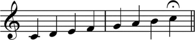
FIGURE 1 Diatonic scale in C.

From these seven diatonic notes, seven diatonic chords are possible. In four-part music, each chord is made up of four voices: soprano, alto, tenor, and bass. The arrangement of these voices produces chords in specific positions and inversions. For the sake of simplicity, the exact procedure for determining chord names and numbers has been omitted.

Notes differ not only by pitch but by duration. The shortest duration FPC handles is the eighth note followed by the quarter note, the dotted quarter note, the half note, the dotted half note, and lastly the whole note. The time signature dictates the number of beats in a measure and what type of note constitutes one beat. For example, in 3/4 time, there are three beats in a measure and a quarter note gets one beat. FPC only considers music in 3/4 or 4/4 time, so a quarter note always gets one beat.

Finally, harmonic rhythm describes the shortest regular chord duration between chord changes. For example, in 4/4 a quarter-note-level harmonic rhythm means that chords change at most every beat. Harmonic rhythm is one of the most important components of traditional four-part analysis, its reliability crucial to correctly identifying chords and chord changes. For this project, only music with quarter-note-level harmonic rhythms was chosen, removing the need to detect harmonic rhythms programmatically.

2 Collecting the pieces—training and test pieces

A collection of four-part MusicXML files was created for use as training and test data by the FPC system. Four-part pieces were collected from Web sites in two different formats: PDF and MusicXML—with the PDFs later converted to MusicXML. A few hymns were entered by hand in Finale 2011, a music notation program capable of exporting to MusicXML.

2.1 Downloading and Converting Files

The two main Web sites used were Hymnary.org and JSBChorales.net. Hymnary is a searchable database of hymns, many of which are offered for download in PDF and MusicXML formats. For the purposes of this project, Hymnary’s PDF files were found to be preferable to its MusicXML files, which were compressed, heavily formatted, and difficult to touch up. A few of the PDFs on Hymnary were simply scans and not native PDFs (ones containing font and character data), so they were entered by hand into Finale 2011 and exported to MusicXML. The other site, JSBChorales.org, offers a collection of Bach chorales entirely in MusicXML format. These MusicXML files were found to be suitable.

XML and PDF files were downloaded from these sites and renamed using the format “title—classifier.pdf” or “title—classifier.xml” where “title” is the hymntune or other unique, harmonization-specific name of the composition and “classifier” is the composer. This naming convention was maintained throughout the project. Individually, the PDF files from Hymnary were converted to MusicXML using a software program called PDFtoMusic Pro. PDFtoMusic Pro is not a text-recognition program, so it can only extract data from PDFs created by music notation software, which all of them were. The free trial version of PDFtoMusic Pro converts only the first page of PDF files, which fortunately created no issue since all but a few of the downloaded hymns were single-page documents. The XML files PDFtoMusic Pro produced carried the xml file extension and were compressed.

2.2 Formatting the MusicXML

Before the XML files could be used, it was necessary to adjust their formatting and, in the case of the XML variety, remove their compression. This was done with Finale. Once open in Finale, lyrics, chord charts, and any extraneous or visually interfering markings were removed manually. If the piece was written in open staff, as was the case with every Bach chorale, a piano reduction (two staves) was created in its place. Measures with pick-up notes were deleted and if beats had been borrowed from the last measure, they were added back. For these reinstated beats, the last chord of the piece was extended.

Any time two layers exist in the same staff of the same measure, FPC expects them to start and finish out the measure together. However, publishers and editors do not like splitting note stems multiple times in a single measure if only one beat requires a split and so tend to add or drop layers mid-measure strictly for appearance (Figure 2). Anywhere these kinds of sudden splits occurred, measures were adjusted by hand (Figure 3).

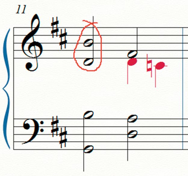
FIGURE 2 Improper layering.

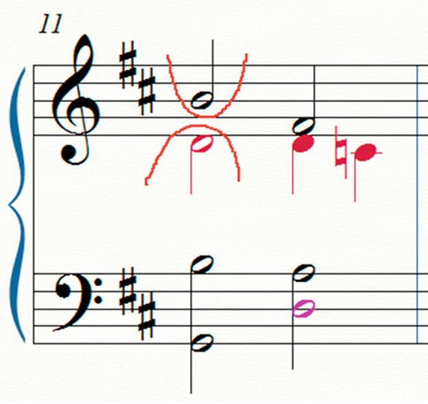
FIGURE 3 Proper layering.

If two parts in the same staff double a note in unison but the staff did not use two layers to do it (Figure 4), the parts were rewritten for that measure (Figure 5). Any rests present were replaced with the corresponding note(s) of the previous chord.

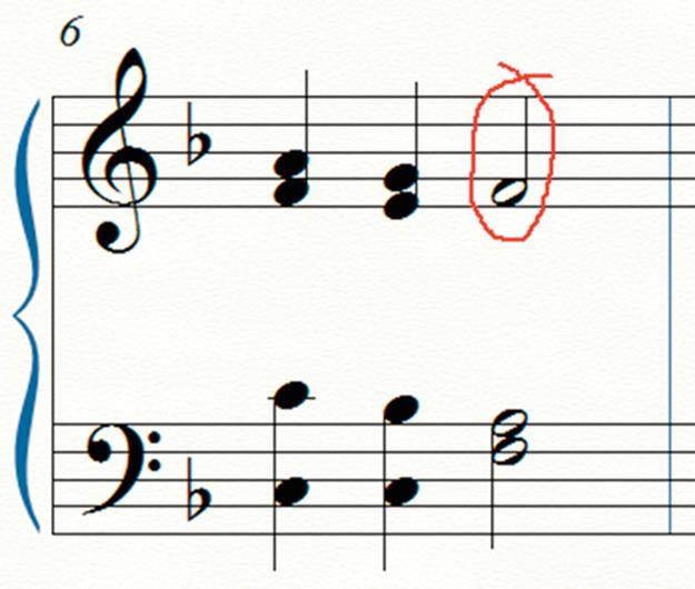
FIGURE 4 Missing layer for presumably doubled note.

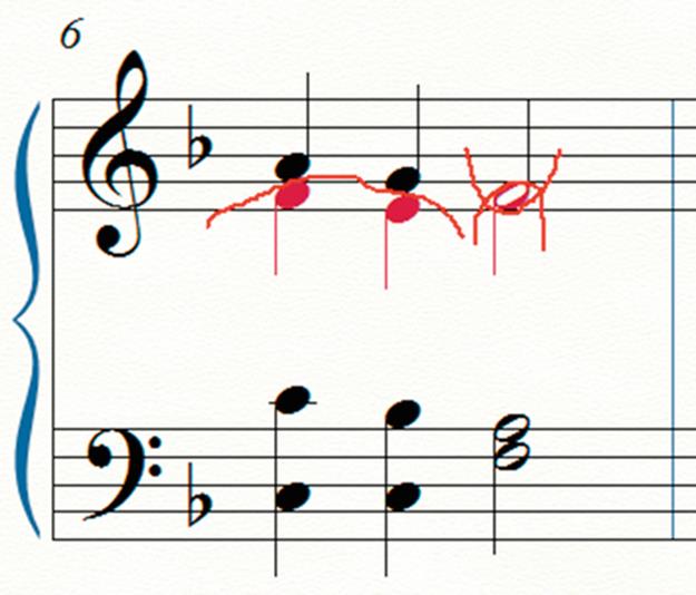
FIGURE 5 Proper layering for doubled note.

Lastly, all measures were copied and pasted into a new Finale document to remove any hidden formatting. The files were then exported with the same naming convention as before and saved in a specific training piece or test piece directory for use by FPC (Figure 6).

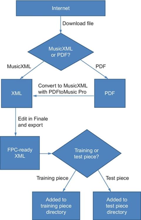
FIGURE 6 Flow chart for collecting pieces.

The next few sections describe how FPC works in general. Section 6 returns to the specific way FPC was used in this experiment.

3 Parsing musicXML—training and test pieces

By clicking the “Load Training XML” or “Load Test XML” button, the user kicks-off step 1 of the data-loading process: Parsing the XML (Figure 7).

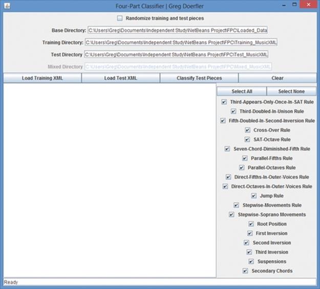
FIGURE 7 FPC upon launch.

3.1 Reading in Key and Divisions

First, FPC parses the key from each file, then the divisions. The number of divisions is an integer value defining quarter note duration for the document. All other note types (half, eighth, etc.) are deduced from this integer and recognized throughout the document. If a quarter note is found to be two, a half note is four.

3.2 Reading in Notes

MusicXML organizes notes by layers within staves within measures. In other words, layer 1 of staff 1 of measure 1 comes before layer 2 of staff 1 of measure 1, which precedes layer 1 of staff 2 of measure 1, and so on. Last is layer 2 of staff 2 of the final measure. If a staff contains only one layer in a particular measure, the lower note of the two-note cluster (alto for staff 1, bass for staff 2) is read before the upper note (soprano or tenor, respectively). Since a measure might contain a staff with one layer and another with two, FPC was carefully designed to handle all possible combinations.

A note’s pitch consists of a step and an octave (e.g., Bb and 3). A hash map is used to relate pitches to integers (e.g., “Bb3” → 18), and these integers are used to represent each voice of a four-part Chord object.

3.3 Handling Note Values

In 3/4 and 4/4 time, a quarter-note-level harmonic rhythm means that chords change at most each beat. Therefore, the chord produced by the arrangement of soprano, alto, tenor, and bass voices at the start of each beat carries through to the end of the beat. This also means that shorter notes moving between beats cannot command chords of their own. Quarter notes, which span a whole beat, are then the ideal notes to capture as long as they fall on the beat, which they always did. Likewise, eighth notes that fall on the beat are taken to be structurally important to the chord, so their durations are doubled to a full beat and their pitches captured, whereas those that fall between beats are assumed to be passing tones, upper and lower neighbors, and other nonchord tones, so they are ignored. For simplicity’s sake, anything longer than a quarter note is considered a repeat quarter note and sees its pitch captured more than once. For instance, a half note is treated as two separate quarter notes and a whole note as four separate quarter notes. A dotted quarter note is assumed to always fall on the beat, so it is captured as two quarter notes; the following eighth note is ignored. While it is possible for something other than an eighth note to follow a dotted quarter, it is highly unlikely in 3/4 or 4/4, and it did not happen in any of the music used.

3.4 Results

Finally, for each XML file, FPC creates a Piece object comprising at the moment a key, classifier, and sequence of Chords. For each piece, it also produces a CSV file with the same information. The CSV files serve purely as logs (Figure 8).

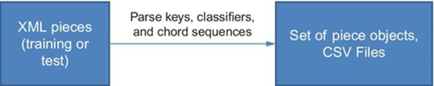
FIGURE 8 Flow chart for creating Piece objects.

4 Collecting Piece Statistics

After the XML has been parsed, FPC moves immediately to the next step: Collecting Piece Statistics.

4.1 Metrics

Statistics are collected for each piece via 19 Boolean tests on each chord or chord change. These Boolean tests produce the following metrics (Diagram 111):

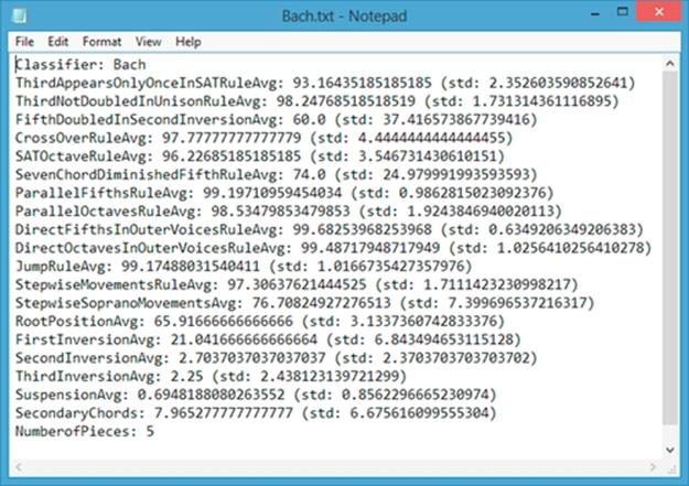
DIAGRAM 111

ThirdAppearsOnlyOnceInSAT The percent of chords whose third appears only once in the upper three voices. In classical writing, it is preferable that the third appear just once in the upper three voices.

ThirdNotDoubledInUnison The percent of chords whose third is not doubled in unison. Doubling the third in unison is usually avoided unless necessary.

FifthDoubledInSecondInversion The percent of second-inversion chords whose fifth is doubled. Classically, it is preferable that the fifth be doubled in second inversion.

CrossOver The percent of chords not containing overlapping parts. It is preferable that voices do not cross over. Doubling in unison is fine.

SETOctave The percent of chords whose soprano and alto pitches as well as alto and tenor pitches differ by not more than an octave. This is a fairly strict rule in classical, four-part writing. The distance between the bass and tenor does not matter and may be great.

SevenChordContainsDiminishedFifth The percent of vii° chords with a fifth. While the fifths of other chords are often omitted, the diminished fifth of a vii° chord adds an important quality and its presence is a strict requirement in classical writing.

NoParallelFifths The percent of chord changes free of parallel fifths. This is a strict rule of classical writing.

NoParallelOctaves The percent of chord changes free of parallel octaves. This is also a strict rule.

NoDirectFifthsInOuterVoices The percent of chord changes free of direct fifths in the outer voices. This is a fairly important rule in classical writing.

NoDirectOctavesInOuterVoices The percent of chord changes free of direct octaves in the outer voices. This also is a fairly important rule.

LeapingParts The percent of chord changes involving a part jumping by a major seventh, a minor seventh, or the tri-tone. Jumping the tri-tone in a nonmelodic voice part is never acceptable in classical writing, but from time to time, leaps by major and minor sevenths and even tri-tones are permissible if in the soprano.

StepwiseMovements The percent of chord changes in which at least one voice moves by no more than a major second. While this is not a formal rule of classical writing per se, good writing generally has very few chord changes in which all four parts leap.

StepwiseSopranoMovements The percent of chord changes in which the soprano moves by not more than a major second.

RootPosition The percent of chords in root position (root in bass).

FirstInversion The percent of chords in first inversion (third in bass).

SecondInversion The percent of chords in second inversion (fifth in bass).

ThirdInversion The percent of chords in third inversion (seventh in bass).

Suspensions The percent of chord changes involving a suspended note that resolves to a chord tone.

SecondaryDominants The percent of chords borrowed from other keys that act as launch pads to chords that do belong in the key (diatonic chords). FPC handles all “V-of” chords (i.e., V/ii, Viii, V/IV, V/V, V/vi) and all “V⁷-of” chords except V7/IV. “V⁷-of” chords are simply recorded as “V-of” chords since they perform the same function.

After all 19 metrics are computed per piece, a TXT file is produced for backup (Figures 9 and 10).

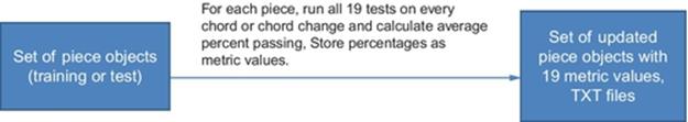
FIGURE 9 Flow chart for collecting Piece statistics.

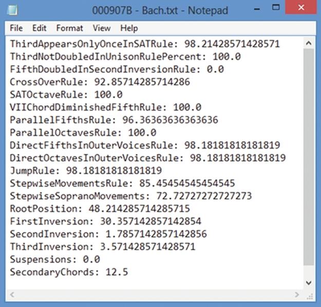
FIGURE 10 Sample TXT file for a Bach chorale containing 19 metric values (percentages).

5 Collecting Classifier Statistics—Training Pieces Only

The previous two steps—Parsing the XML and Collecting Piece Statistics—apply to the loading of both training and test data. Step 3, however, applies to training data only. If the user has clicked “Load Training XML,” FPC now begins the final step before it is ready to start classifying test pieces: Collecting Classifier Statistics.

In the sections that follow, “classifier” with a lowercase “c” refers to the Piece object’s string field while “Classifier” with a capital “C” refers to the Classifier object.

5.1 Approach

For each training piece belonging to the same classifier, a Classifier object is created. The mean and standard deviation are computed for each metric from all the pieces of the classifier and then stored in the Classifier object. For any piece, metrics outside three standard deviations of the mean are thrown out, and the means and standard deviations are recalculated. Again, the whole piece is not thrown out, just the piece’s individual metric(s). FPC updates each Classifier object with the new mean(s) and standard deviation(s) and then produces TXT files with the same information. Figure 11 provides an example to illustrate the process.

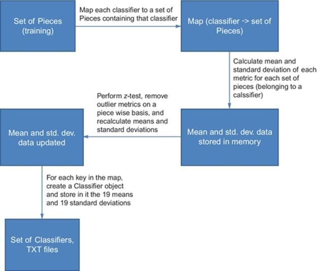
FIGURE 11 Flow chart for collecting Classifier statistics.

Example: Pieces 1–10 belong to Classifier A, Pieces 11–20 to Classifier B, and Pieces 21–30 to Classifier C. The mean for metric X from Pieces 1–10 is calculated to be 15 (as in 15%) and the standard deviation is 5 (as in 5% points). If Piece 10’s metric X is 31, which is greater than 15 + 3 × 5 (z-test upper-bound), it is an outlier. Piece 10’s metric X is therefore discarded and the mean and standard deviation for metric X are recomputed using Pieces 1–9. Classifier A then receives the new mean and standard deviation for metric X, and a TXT file is written. These steps are repeated for Classifiers B and C.

6 Classifying Test Pieces

Three techniques were used to classify test pieces from metric data: Unweighted Points, Weighted Points, and Euclidean Distance.

6.1 Classification Techniques

Unweighted Points is the simplest technique. It treats each metric equally, assigning a single point to a Classifier each time one of its metrics best matches the test piece. The classifier with the most points at the end is declared the winner and is chosen as the classification for the test piece.

Weighted Points was an original approach. It works similar to Unweighted Points except metrics can be worth different amounts of points. First, it calculates metric differences from the Classifiers: For each metric, it finds the Classifier with the highest value and the one with the lowest value. It subtracts the lowest value from the highest value, and the difference becomes the number of “points” that metric is worth. Then, like Unweighted Points, it looks to see which Classifier is closest to the test piece for each particular metric, only instead of assigning a single point, it assigns however many points the metric is worth.

Euclidean Distance is a standard technique for calculating distances in high-dimensional space. Here, it focuses on one Classifier at a time, taking the square root of the sums of each metric difference (between test piece and classifier) squared. This is illustrated inFigure 12, where p is the classifier, q is the test piece, and there are n metrics.

FIGURE 12 Euclidean distance formula.

Euclidean distance is calculated for each classifier, and the classifier with the smallest distance from the test piece is chosen as the classification.

6.2 User Interface

A row of four buttons allows the user to load training XML, load test XML, classify test pieces, and clear results. Above these buttons sit textboxes displaying the paths to files FPC will read or write on the user’s machine during use. At the very top of the UI is a checkbox allowing FPC to select the training and test pieces from the collection randomly. Randomizing training and test pieces requires XML to be loaded each time a trial is run (since Classifiers will likely contain different data). Therefore, checking this box disables the “Load Training XML” and “Load Test XML” buttons, moving their combined functionality into the “Classify Test Pieces” button. Below the row of buttons is an information area, which displays the results of each step including test piece classification. To the right of the information area can be found a panel of checkboxes giving the user control over the metrics. Metrics can be turned on or off to help the combinations producing the most accurate results be discovered. At the very bottom of FPC sits a status bar that reflects program state.

6.3 Classification Steps

When the user clicks “Classify Test Pieces,” test piece data from the TXT files created in step 2 (collecting piece statistics) are read and loaded into memory. It is true that if the user has performed steps in the normal order and loaded training XML before test XML, the test piece data would still be in memory, and reading from file would not be necessary. However, due to the sharing of Piece objects between training pieces and test pieces, if steps were done out of order, the Piece objects, if still in memory, might contain training data instead of test data. And because each TXT file is small, reading in the data proves a reliable way to ensure good system state if, for example, the user were to load training and test data, exit the program, and launch FPC again hoping to start classifying test pieces immediately without reloading. Here, reading from files is the simplest solution.

Next, if the Classifiers are not already in memory, the data are read in from the Classifier TXT files produced in step 3 (collecting classifier statistics). For each test piece, its metric values are compared with those of each Classifier. Each classification technique then scores the metrics and handles the results in its own, unique way.

6.4 Testing the Classification Techniques

Four-part music was selected comprising three composers: J.S. Bach, John Bacchus Dykes, and Henry Thomas Smart. Dykes and Smart were nineteenth century English hymnists, while Bach was an early eighteenth century German composer. Dykes and Smart were chosen for their similarities with one another, while Bach was chosen for his differences from them.

Using all 19 metrics, 20 trials were run per composer combination: (1) Bach versus Dykes, (2) Bach versus Smart, (3) Dykes versus Smart, and (4) Bach versus Dykes versus Smart. The averages were then computed for each classification technique. Later, 20 more trials were run for Bach versus Dykes using a subset of metrics thought most important.

Forty-five pieces in all were used—15 per composer—and randomization was employed on each trial so that training pieces and test pieces could be different each time.

6.5 Classifying from Among Two Composers

For all three evaluation techniques, the averages of each trial, when classifying among two composers, came out well above 50%—the value expected from a two-composer coin toss. In fact, no individual trial fell below 50%.

Bach Versus Dykes—All Metrics

Bach Versus Smart—All Metrics

Dykes Versus Smart—All Metrics

The best technique overall was Weighted Points, demonstrating the strongest performance in two out of the three classifications.

6.6 Classifying from Among Three Composers

For all three evaluation techniques, the averages of each trial, when classifying among three composers, came out well above 33.3%—the value expected from random, three-way guessing. In fact, no individual trial dipped below 33.3%. The technique that worked best was Unweighted Points followed by Weighted Points at a close second.

Back Versus Dykes Versus Smart—All Metrics

6.7 Selecting the Best Metrics

If all 45 pieces were to be used to train the system, the resulting classifier data would represent what data from a randomized trial would look like on average. In this case, one can see that Bach’s chord inversion statistics are far different from those of Dykes and Smart. Bach also relies more heavily on secondary chords:

Classifier Data from 45 Test Pieces

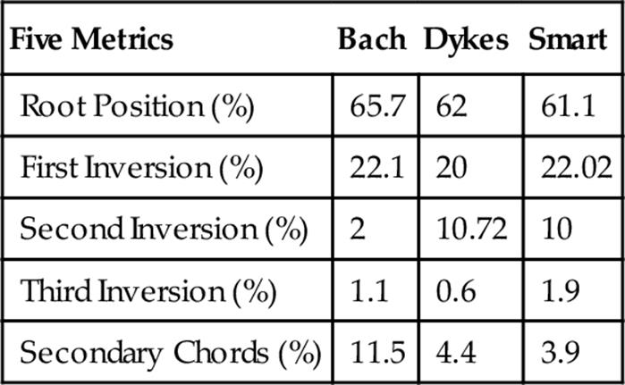
To test if FPC could even more accurately distinguish between Bach and either of the others, 20 additional trials were run for Bach and Dykes using only root position, first inversion, second inversion, third inversion, and secondary chords metrics.

Bach Versus Dykes—Five Metrics

Although Unweighted Points was 1.8% points less accurate, Weighted Points improved by 1.8% points, and Euclidean Distance was a surprising 17.8% points more accurate. Whereas Euclidean Distance performed the worst last time, this time it actually performed the best. Using only these five metrics likely removed considerable amounts of “noisy” data, which suggests Euclidean Distance performs best with low noise.

7 Additional Composer and Metrics

Later, a fourth composer, Lowell Mason, was added as were three more metrics with similarities to the five metrics that had performed the best so far. The new metrics were introduced to see if they could rival those five metrics or supplement them.

7.1 Lowell Mason

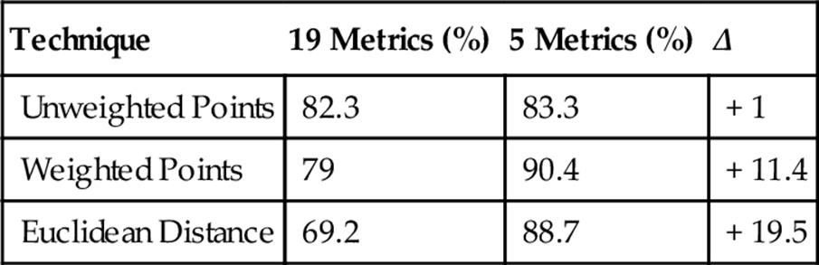
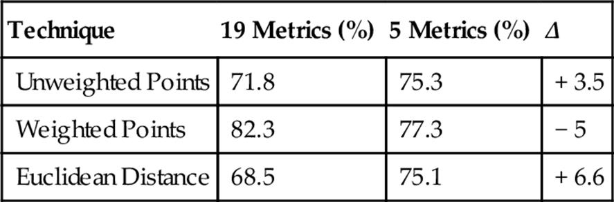
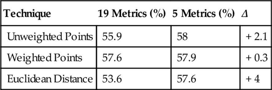
Before introducing the three new metrics, it was intriguing to see if the five metrics from before continued to dominate the other 14 metrics when Mason was added. Covering all 7 of the newly possible composer combinations (BM, DM, SM, BDM, BSM, DSM, and BDSM), 140 additional trials were run (20 per combination) for the original 19 metrics and again for the 5-metric subset.

Bach Versus Mason

Dykes Versus Mason

Smart Versus Mason

Bach Versus Dykes Versus Mason

Bach Versus Smart Versus Mason

Dykes Versus Smart Versus Mason

Bach Versus Dykes Versus Smart Versus Mason

As seen above, the results with Mason were in keeping with the correctness levels of previous classifications, and as a whole, the five-metric subset continued to perform better than the entire set of metrics. Not surprisingly, the percent of correct answers (for all techniques and both metric sets) was overall at its lowest in the last set of trials, when all four composers were classified together. However, the percentages were well above 25% and statistically appropriate for the change from three to four composers based on past three-way classifications. They were actually much better than expected.

A look through the classifier data produced during these seven classifications revealed that Mason had a very high ThirdAppearsOnlyOnceInSAT percentage compared to the other composers, yet a relatively low standard deviation. This raised the question of whether the ThirdAppearsOnlyOnceInSAT metric was worth adding to the special set of five metrics, so the last classification was rerun to include it. Consequently, results saw a significant 3–4% point improvement, suggesting this to be another helpful metric worth isolating in the future.

7.2 Additional Metrics

Because the five metrics that were isolated proved so useful, three new metrics were developed to analyze similar musical features. The metrics are as follows:

OpenPosition The percent of chords considered “open” by music theory standards. In an open chord, at least one chord tone is skipped over between soprano and alto, and alto and tenor.

ClosedPosition The percent of chords considered “closed” by music theory standards. Generally, the soprano, alto, and tenor are packed together as tightly as possible in a closed chord.

SameChordNumberDifferentInversion The percent of chord changes in which the chord number remains the same but the inversion changes.

Like in previous classifications, the new metrics were used to classify music by all four composers in groups of two, three, and four composers at a time. The new metrics were tested on their own, in combination with the five-metric subset, and in combination with the original 19 metrics.

Interestingly, in most cases FPC was less accurate than previously in its classifications. Accuracy actually suffered the most when these three metrics were used in conjunction with the five metrics that had previously performed best. Although these new metrics were aimed at imitating the properties of the ones that had been so successful, they failed to add any value.

8 Conclusions

It has been shown how FPC uses metrics based on chord structure and chord movement as input for three classification techniques. Furthermore, it has been demonstrated that conducting multiple randomized trials with test pieces of known classification allows the accuracy of FPC’s guesswork to be easily measured.

Analyzed results from multiple trials indicate FPC is most reliable when only a handful of the most effective metrics are used. Root position, first inversion, second inversion, third inversion, and secondary chords metrics have proven, at least here, to be the most important factors in distinguishing between composers. A logical direction for future work would be to test FPC’s performance classifying four-part music by time period instead of composer.

References

[1] Ebcioglu K. An expert system for chorale harmonization. In: AAAI-86 Proceedings; 1986:784–788. http://www.aaaipress.org/Papers/AAAI/1986/AAAI86-130.pdf.

[2] Nichols E, Morris D, Basu S. Data-driven exploration of musical chord sequences. In: Proceedings of the 14th international conference on Intelligent user interfaces (IUI’09). ACM, New York, NY, USA; 2009:227–236. doi:10.1145/1502650.1502683.

[3] Doerfler G, Beck R. An approach to classifying four-part music. In: Proceedings of the 2013 International Conference on Image Processing, Computer Vision, and, Pattern Recognition (IPCV); 2013:787–794.

Further reading

Anders T, Miranda ER. Constraint programming systems for modeling music theories and composition. ACM Computing Surveys. 2011;43(4):doi:10.1145/1978802.1978809. Article 30 (October 2011), 38 pages. http://doi.acm.org/10.1145/1978802.1978809.

De Prisco R, Zaccagnino G, Zaccagnino R. EvoBassComposer: a multi-objective genetic algorithm for 4-voice compositions. In: Proceedings of the 12th Annual Conference on Genetic and Evolutionary Computation (GECCO '10). ACM, New York, NY, USA; 2010:817–818. doi:10.1145/1830483.1830627.

Edwards M. Algorithmic composition: computational thinking in music. Comm. ACM. 2011;54(7):58–67. doi:10.1145/1965724.1965742.