Emerging Trends in Image Processing, Computer Vision, and Pattern Recognition, 1st Edition (2015)

Part I. Image and Signal Processing

Chapter 3. Measuring rainbow trout by using simple statistics

Marcelo Romero; José Manuel Miranda; Hector A. Montes-Venegas Facultad de Ingeniería, Universidad Autónoma del Estado de México, Toluca, Estado de México, Mexico

Abstract

Traditionally, a manual method is used to classify the rainbow trout in small farms, which generally cause stress and physical damage to the fish. Additionally, this manual classification is not always accurate, as farmers only visually check whether the trout is fry, fingerling, or table-fish size. In this article, we robustly evaluate our simple statistical system to measure rainbow trout in farms. For this research, we have designed and implemented a novel prototype that includes canalization, illumination, and vision components to take a 2D downward-view image of the trout. After that, this image is processed to get the trout’s contour, which is used to estimate the fish’s length by adjusting the best regression curve to this contour. Finally, the trout’s size is defined by the minimum Mahalanobis distance to training data. We have evaluated our experimental results as a binary classification problem and the best precision scores are 95.93%, 93.21%, and 96.25% when classifying fry, fingerling, and table-fish trout, respectively. These experimental results are computed by using our state-of-the-art database of 1800 rainbow trout images, which was collected with our physical prototype for this publication.

Keywords

Rainbow trout measuring

Statistical measuring

Fish classification

Acknowledgments

Authors thank to the Research Department of the Autonomous University of the State of Mexico (UAEMex) for its financial support through the research project SIyEA/32742012 M. Their gratitude also goes to the Mexican Council for Science and Technology (CONACyT) for the scholarship granted to Jose Manuel Miranda (634478).

1 Introduction

Generally, small farms use a manual measuring and counting process when cultivating rainbow trout [1–4]. There are many reasons to perform such classification, but the most important are to feed the trout according to its size and to avoid cannibalism into the tanks [4]. Problems when doing a manual classification are, indistinctively, the stress and physical damage causes to the specimen when manipulated by the farmer. Moreover, we believe that this classification approach is not accurate, where the trout is taken from the water using a net and visually the farmer decide whether or not the trout should be changed to another tank.

Mexico, as well as many other countries in the world, has large hydric areas, which are ideal for aquaculture [5,6]. Taking advantage of both, its altitude and natural water resources, the State of Mexico (Mexico) has particular interest in increasing the trout’s production as a sustainability and economic strategy for local small farmers [7]. Hence, this is a good opportunity to integrate technology to optimize the trout’s production in this region.

That is the reason which motives our research interest in the field, where we have accomplished some results, including a research project [3] and a couple of bachelor in science dissertations [1,2]. In this paper we robustly evaluate our experimental procedure to measure rainbow trout [8] in a small farm located in the Valley of Toluca, Mexico [9], where we have observed a manual classification process as illustrated in Figure 1.

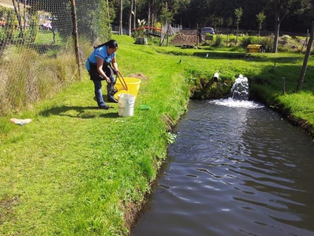
FIGURE 1 Manual measuring-classification process generally done in small farms in central Mexico. Note that this small farms use lined earth tanks.

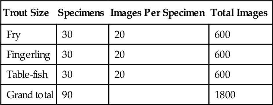
Therefore, robust experimental results are presented in this publication by using our statistical system [8] and a state-of-the-art rainbow trout image database specially collected for this article. These data corpus were collected by capturing 20 images for each of 30 specimens per size (fry, fingerling, and table-fish), counting 1800 rainbow trout images.

Some related work is observed in the literature. Hsieh et al. [10] proposed a technique to measure dead tuna fish using a colour pattern. In this work, the fish length is estimated by proportional relationship between the fish body pixel length and an image reference scale. Ibrahim and Wang [11] measure four dead fish classes by constructing a central line along the fish body from horizontal and vertical views of the fish’s body. Finally, a commercial counting and measuring system is observed in Vaki System [12]; however, there is no further information about its classification procedure.

The rest of this article is as follows. First, Section 2 describes our novel prototype designed for this research. Then, Section 3 introduces our statistical measuring approach. After that, Section 4 details our experimental framework. Next, Section 5 shows our performance evaluation. Finally, Section 6 concludes this article and draws some venues for our future work.

2 Experimental prototype

In this section, we describe our experimental prototype, which has been designed as part of this research.

This novel prototype is essential to collect useful trout’s 2D images; therefore, we have meticulously designed it. Figure 2 shows our experimental prototype, which has evolved from a traditional squared glass fish-cube (prototype version 1). We observed relevant issues from our first prototype and that knowledge was experimentally analyzed to obtain our second model. Note that our two prototypes have been experimentally evaluated in a trout farm; so, we have gathered special knowledge about handling the rainbow trout.

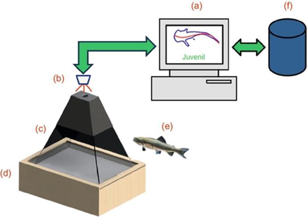
FIGURE 2 Our experimental scenario for measuring rainbow trout. (a) Statistical approach within a personal computer, (b) vision system, (c) canalization system, (d) illumination system, (e) specimen to be measured, and (f) database.

Then, as observed in Figure 2, our experimental prototype consists of three main components: canalization, illumination, and vision which are aim to collect RGB trout images using a standard personal computer.

2.1 Canalization System

We have design a novel canalization system based on opaque-glass within our prototype. This canalization system poses two main properties. The first property is regarded to its trapezoidal shape, which has been decided according to the digital camera’s vision field principle. As long as such trapezoidal shape avoids reflection to be captured when taking a digital image. As its second property, we can mention that this is a two-canal tray, which prevents occlusion by taking only one fish per canal and it allows capturing two rainbow trout images per shot.

2.2 Illumination System

To assist our vision system, we have integrated an illumination system, which distributes light in a uniform way at the bottom of the canalisation system. To do this, a light source is located to an appropriate high to distribute light uniformly over an acrylic diffuser. The light-source’s high was defined by using a bisection approach and measuring the light intensity projected into the diffuser with photo resistors. We integrated this diffuse illumination to increase contrast into the image and highlighting the trout’s body.

2.3 Vision System

In order to explore economical technology for our classification system, we have used a standard 2D LifeCam Studio [13] camera in this experimentation. This camera is able to capture RGB-images with a maximum resolution of 1920 × 1080 pixels. In this prototype, this RGB camera is located at the top of the canalization system to capture downward-view images of the trout. Its high is proportional to the canalization base length to avoid extra data to be captured.

3 Statistical Measuring Approach

In this section, we present our statistical approach to measure rainbow trout.

Considering the rainbow trout natural swimming movement against the water flow and observing the trout from a downward point of view, we hypothesized that a third- order curve could approximate the trout’s body within the water.

Different procedures can be followed to obtain a third-order curve equation. However, we prefer a simple but effective solution that could be executed online after a trout’s image is captured.

Then, given n sample points (x,y) which depict the trout body, we apply minimum squares to compute a polynomial third-order equation [14]:

(1)

where a₀, a₁, a₂, a₃ are constants that gain their values by solving the [4 × 4] equation system 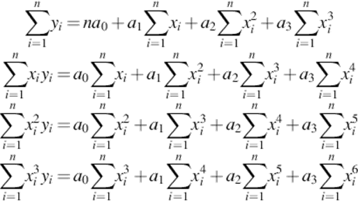(2):

(2)

The equation system (2) can be easily solved using the matrix notation, AX = B, or more specifically: X = BA^{− 1}.

After this computation, we obtained the best regression curve that adjusts the trout’s body captured into an RGB image.

Then, we observe that this regression curve is related to the trout’s length, which could be estimated by computing the Euclidean distance among the points within the regression curve.

Finally, given a probe-length (l_i) a classification can be done by comparing against training lengths. For this research, such comparison is performed by computing the Mahalanobis distance [15] from training fry, fingerling, and table-trout lengths:

(3)

Hence, a probe-trout t_i is classified through its estimated length l_i by comparing its Mahalanobis distance d_i against a predefined threshold, which in fact is the number of standard deviations that is expected to be to the training mean length ().

4 Experimental framework

This section presents the experimental framework to illustrate how rainbow trout is measured using our statistical approach.

As show in Figure 3, after an RGB image is taken by our prototype, we are following a five-stage image processing to get the trout’s contour. As explained in Section 3, we are measuring the trout’s length using this contour.

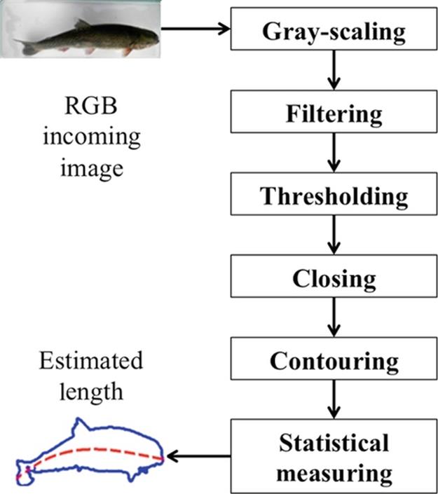
FIGURE 3 Processing an incoming RGB image to estimate the trout’s length using our statistical approach.

To classify the trout’s image within an image, we are performing four main steps. Firstly, an RGB image of the trout is taken using our prototype (Section 2). Secondly, this RGB image is processed to obtain the trout’s contour. Thirdly, the trout’s length is estimated by applying our statistical method (Section 3) to the trout’s contour. Finally, using that estimated length, the trout is classified using a binary classification approach.

In Section 4.1, we provide more detail about our image processing step.

4.1 Testing Procedure

As illustrated in Figure 2, we have implemented a novel functional prototype which allows us to gather RGB images. After that, as shown in Figure 3, RGB images are processed using standard algorithms in the literature [16,17] until we obtain the trout’s contour. Next, we apply our statistical approach to that contour, so we can estimate the trout’s length. Finally, a binary classification approach is taken to classify the trout within the income image. We now detail our experimental procedure:

1. As mentioned before, we have collected a trout-image database using our prototype (illustrated in Figure 4) in a farm. This database was created using 30 fry, 30 fingerling, and 30 table-fish specimens, capturing 20 images per specimen. This state-of-the-art rainbow trout image database (see Table 1) was recently collected for this publication. However, for this experiment we are using only 450 images per size.

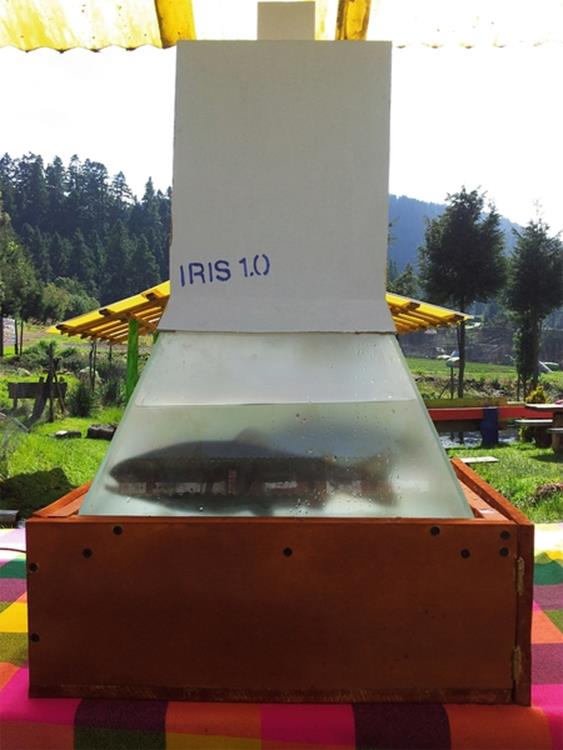
FIGURE 4 Functional prototype used within our measuring system. This prototype includes an illumination source, a pyramidal canalization compartment and a 2D camera.

Table 1

Experimental Data Images

2. From our database, separate training and testing sets are defined (see Table 2). Thus, 450 images for training and 900 images for testing are used. Specifically, we have three training data sets, containing 150 images per size, namely, fry, fingerling, and table-fish trout. In every case, we selected the first five-captured images for each of the 30 specimens per size to be part of the training set. Then, we use the next 10-captured images for each of the 30 specimens for testing. By doing this, we have three testing sets (one per trout-size) containing 300 images of fry, fingerling, and table-fish, respectively.

Table 2

Training and Testing Sets

3. From these 450 training images, training data are gathered, which in fact consist of training lengths, the arithmetic mean, and the standard deviation for each size.

4. For each testing trout image, estimated lengths are gathered as illustrated in Figures 3 and 5. To do this, we gather an RGB image using our prototype. Then, we execute a five-stage image processing: gray-scaling, filtering, thresholding, closing, and contouring. Next, we estimate the trout’s length by applying our statistical approach to the contour obtained above. Finally, using this estimated length we classify the trout as fry, fingerling, or table-fish.

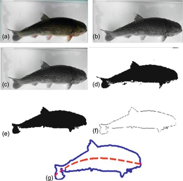
FIGURE 5 Image processing performed to measure a rainbow trout using our statistical approach. (a) RGB incoming image sensed by the vision system; (b) gray-scaling; (c) filtering; (d) thresholding; (e) closing; (f) contouring; and (g) trout’s length estimated by a third order regression curve (plotted as dash line).

5. To speed up our image-processing step, our vision system gathers [640 × 360] pixels RGB-images.

6. Captured RGB values are converted into a grayscale by forming weighted sums of the R, G, and B components [16]:

(4)

7. Noise reduction is performed in every grayscale image by using a [3 × 3] Gaussian low-pass filter and σ = 0.6

(5)

8. A binary image is obtained by using a 0.245 threshold, which was calculated experimentally from training rainbow trout images.

9. The trout’s body is emphasized by using a closing operation, first erosion, and then dilation with a [5 × 8] mask. This operation is the key to eliminate small clusters of pixels around the trout’s body cluster.

10. The trout’s contour is obtained by removing interior pixels. In this case, a pixel is set to 0 if all its four-connected neighbours are 1, thus leaving only the boundary pixels on as shown in Equation 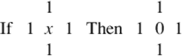(6):

(6)

11. Using the trout’s contour, we apply our statistical measuring approach detailed in Section 3.

12. By definition, the trout’s size is estimated by computing the Mahalanobis distance from this estimated length to training data (Equation 3).

13. For classification in this experiment, imagine that the complete testing-trout set (900 in total) is passed through a grid one by one in three steps. First, the grid is sized to filter only fry-trout. Then, every trout able to pass this grid is labelled as a fry-trout. Second, for the rest of the testing set, the grid is now sized to filter fingerling-trout. Every trout that is able to pass this grid is labelled as fingerling-trout. Third, for the rest of the testing set, the grid is now sized to filter table-fish trout.
Remember that we are computing the Mahalanobis distance and this allows us to easily implement the approach above using fry, fingerling, and table-fish training data, respectively. Referring as training data the arithmetic mean and the standard deviation from each size.
Another advantage in using Mahalanobis distance is that we can make our classification process as rigid as we decide, by defining a threshold in number of standard deviations.
Then, in this article we are reporting classification figures from one to three standard deviations.

14. We are considering this experiment as a binary classification problem, as illustrated in Table 3. By doing this, we are collecting true positive (TP), false positive (FP), false negative (FN), and true negative (TN) frequencies [18].

Table 3

Binary Classification

15. Using values in Table 3, performance figures are generated by computing accuracy, repeatability, specificity, recall, and precision metrics when classifying as fry, fingerling, and table-fish trout. In every case, we are evaluating using as threshold from one to three standard deviations.
Accuracy, a degree of veracity, is a measurement of how well the binary classification test correctly identifies a rainbow trout’s size.

(7)

Repeatability, a degree of reproducibility, is an indicator about how robustly a rainbow trout size can be identified:

(8)

Specificity, a degree of speciality, rates how negative rainbow trout’s size is correctly identified:

(9)

Recall measures the fraction of positive examples that are correctly labelled:

(10)

Precision measures that fraction of examples classified as positive that are truly positive:

(11)

5 Performance evaluation

We now present performance figures when using our statistical model to measure rainbow trout in a farm.

As observed in Figure 5, our statistical approach’s performance to measure a rainbow trout depends on our image processing stage. However, according to our experimental results, we believe that we have addressed main issues about capturing and processing an RGB image within our system.

As we have mentioned before, we consider this as a binary classification problem as indicated in step 13 in our experimental procedure (Section 4.1). Thus, the complete testing lengths (computed from 900 images) are compared against fry training data, using Mahalanobis distance. Then, if a testing length falls into a predefined threshold (one to three standard deviations), the respective testing trout is marked as fry-trout. Next, all remaining testing lengths are compared against fingerling training data using Mahalanobis distance as well. Again, if the testing length falls into a predefined threshold (one to three standard deviations), we label the respective testing trout as fingerling-trout. Then, every remaining testing length is compared against table-fish training data using Mahalanobis distance. Similarly, if the testing length falls into a predefined threshold (one to three standard deviations), the testing trout is labelled as table-fish-trout.

Then, as prescribed in Table 3 we count TP, FP, TN, and FN frequencies, which are summarized from Tables 4 to 6. Hence, by using these values we are able to compute accuracy, repeatability, and specificity metrics, which are presented from Tables 7 to 9 and illustrated in Figure 6.

Table 4

Frequency when Classifying a Probe Set as Fry Trout at Three Standard Deviations

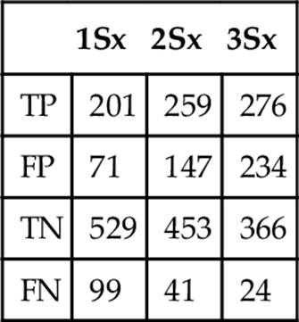
Table 5

Frequency when Classifying as Fingerling Trout at Three Standard Deviations

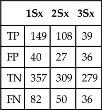
Table 6

Frequency when Classifying as Table-Fish Trout at Three Standard Deviations

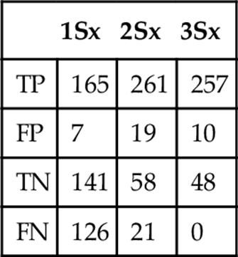
Table 7

Accuracy when Classifying a Probe Set at Three Standard Deviations

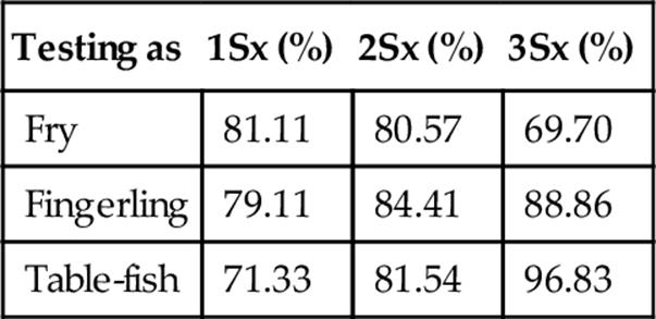
Table 8

Repeatability when Classifying a Probe Set at Three Standard Deviations

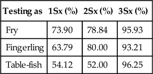
Table 9

Specificity when Classifying a Probe Set at Three Standard Deviations

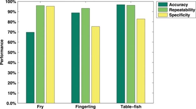
FIGURE 6 Accuracy, repeatability, and specificity performance when classifying fry, fingerling, and table-fish trout at three standard deviations using our statistical measuring system.

Finally, we are computing recall and precision metrics. Tables 10 and 11 summarize these results and Figure 7 shows recall and precision results at three standard deviations.

Table 10

Recall when Classifying Testing Sets at Three Standard Deviations

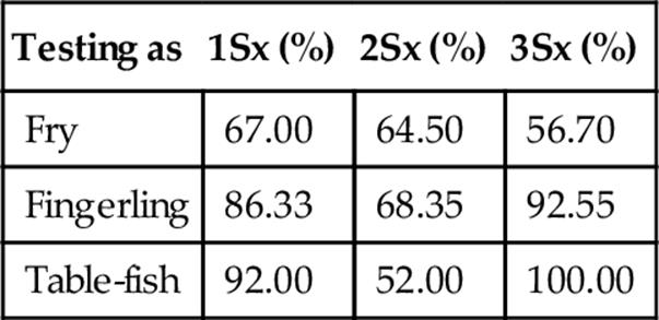
Table 11

Precision when Classifying Testing Sets at Three Standard Deviations

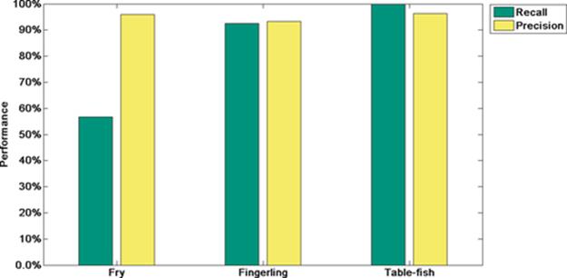
FIGURE 7 Recall-precision metrics when classifying fry, fingerling, and table-fish trout at three standard deviations using our statistical measuring system.

Observing our experimental results when classifying our testing set, we score the best precision at three standard deviations: 95.93%, 93.21%, and 96.25% for fry, fingerling, and table-fish trout, respectively.

Furthermore, when classifying those testing lengths, we score a 100% recall and 96.25% precision when classifying table-fish trout at three standard deviations.

These experimental results are not only motivated, but also valuable evidences that indicate effectiveness in our classification system.

6 Conclusions

In this article, we have robustly evaluated our statistical system to measure rainbow trout in farm using computer vision as observed in Figure 8. This novel technique [8] is a simple but effective statistical method, which has been evaluated in a small farm in central Mexico named Rincon del Sol [9].

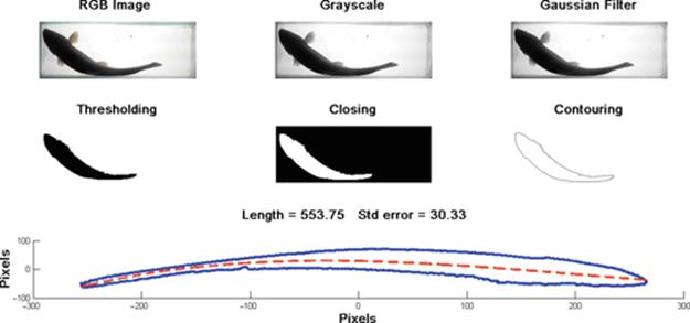
FIGURE 8 Processing a table-fish trout image for classification using our statistical measuring system.

For this research, we have designed and implemented a functional prototype to collect RGB trout images. This prototype includes canalization, illumination, and vision components that have been meticulously assembled. Also, we believe that this prototype could be easily integrated into a mechanical system to interconnect lined earth tanks in farms.

Our experimental results encourage our research as they have shown that our classification system is effective, where 95.93%, 93.21%, and 96.25% precisions are observed when classifying fry, fingerling, and table-fish trout, respectively.

It is important to observe that, although our statistical approach has been inspired to measure rainbow trout, this approach can be applied to other fishes grown in farms.

As part of our future work, we are integrating water flow and stereovision into our prototype to investigate two main issues: the light reflection into the water and the presence of turbulence. Our final aim is to implement an economical classification system for small farms.

References

[1] Mejia S. Conteo y clasificación de la trucha arcoíris utilizando visión artificial: revisión literaria y análisis [BSc. Final dissertation]. Mexico: Engineering Department, Autonomous University of the State of Mexico; 2013.

[2] Miranda J. Prototipo de un sistema clasificador de la trucha arcoíris utilizando un modelo estadístico de su longitud obtenido de imágenes 2D [BSc thesis]. Mexico: Engineering Department, Autonomous University of the State of Mexico; 2014.

[3] Romero M, Vilchis A, Portillo O. Intelligent system to count, measure and classify fishes using computer vision. Research project SIyEA 32742012 M. Mexico: Autonomous University of the State of Mexico; 2012.

[4] Woynarovich A, Hoitsy G, Moth-Poulsen T. Small-scale rainbow trout farming. FAO Fisheries and aquaculture technical paper, Food and Agriculture Organization of the United Nations; 2011.

[5] CONAGUA, Comisión Nacional del Agua. Concesión de Aprovechamiento de Aguas Superficiales. Water National Council; 2006. [Online] Available from: http://www.conagua.gob.mx/Contenido.aspx?n1=5&n2=101&n3=302&n4=302. [Accessed: 13 September 2014].

[6] DOF, Diario Oficial de la Federación. Ley de aguas nacionales. DCVII(14): 27–95. Federal Oficial News. [Online] Available from: http://dof.gob.mx/nota_detalle.php?codigo=670229&fecha=12/05/2004. [Accessed: 13 September 2014]; 2004.

[7] Gallego I, Carrillo R, Garcı´a D, Sasso I, Guerrero J, Burrola C, et al. Programa maestro, sistema producto trucha del Estado de Me´xico. Government Plan for Rainbow Trout Production. Mexico: Autonomous University of the State of Mexico; 2007.

[8] Romero M, Miranda JM, Montes HA, Acosta JC. A statistical measuring system for rainbow trout. In: Proceedings on the international conference on image processing, computer vision and pattern recognition. Las Vegas NE, United States of America; 2014.

[9] Rincon del Sol. Small Trout Farm. La Marqueza, State of Mexico, Mexico; 2014. [Visited: 20 August 2014].

[10] Hsieh C, Chang H, Chen F, Liou J, Chang S, Lin T. A simple and effective digital imaging approach for tuna fish length measurement compatible with fishing operations. Comput Electron Agric. 2011;75:44–51.

[11] Ibrahim M, Wang J. Mechatronics applications to fish sorting part 1: fish size identification. industrial electronics (ISIE 2009). In: IEEE international symposium; 2009.

[12] Vaki System. Bioscanner Fish Counter. [Online] Available from: http://www.vaki.is/Products/BioscannerFishCounter/. [Accessed: 10 May 2014]; 2013.

[13] LifeCam Studio. LifeCam Studio. [Online] Available from: http://www.microsoft.com/hardware/en-us/p/lifecam-studio. [Accessed: 13 September 2014]; 2014.

[14] Murray S, Schiller J, Srinivasan R. Probability and Statistics. 4th ed. USA: Mc Graw-Hill; 2012.

[15] Duda R, Hart P, Stork D. Pattern classification. 2nd ed. USA: Wiley Interscience; 2001.

[16] Gonzales R, Woods R. Digital image processing. 3rd ed. USA: Prentice Hall; 2008.

[17] Gonzales R, Woods R, Eddins S. Digital image processing using Matlab. 2nd ed. USA: Prentice-Hall; 2009.

[18] Davis J, Goadrich M. The relationship between precision-recall and ROC curves. In: Proceedings of the 23rd International Conference on Machine Learning; 2006.