R Data Mining Blueprints (2016)
Chapter 9. Applying Neural Network to Healthcare Data
Neural-network-based models are gradually becoming the backbone of artificial intelligence and machine learning implementations. The future of data mining will be governed by the usage of artificial neural-network-based advanced modeling techniques. One obvious question: why is neural network gaining so much importance recently though it was invented in 1950s? Borrowed from the computer science domain, a neural network can be defined as a parallel information processing system where the inputs are connected with each other like neurons in the human brain to transmit information so that activities such as face recognition, image recognition, and so on can be performed. In this chapter, we are going to learn about application of neural-network-based methods in various data mining tasks such as classification, regression, time series forecasting, and feature reduction. Artificial Neural Network (ANN) functions in a way that is similar to the human brain, where billions of neurons link to each other for information processing and insight generation.
In this chapter, you will learn about various types of neural networks, methods, and variants of neural networks with different functions to control the training of artificial neural networks in performing standard data mining tasks such as:
· Prediction of real valued output using regression-based methods
· Prediction of output levels in a classification-based task
· Forecasting future values of a numerical attribute based on historical data
· Compressing features to recognize important ones in order to perform prediction or classification
Introduction to neural networks
The brain's biological network provides the basis for connecting elements in a real-life scenario for information processing and insight generation. It's a hierarchy of neurons connected through layers, where the output of one layer becomes the input for another layer; information passes from one layer to another layer as weights. The weights associated with each neuron contain insights so that the recognition and reasoning become easier for the next level. Artificial neural network is a very popular and effective method that consists of layers associated with weights. The association between different layers is governed by a mathematical equation that passes information from one layer to the other. In fact, a bunch of mathematical equations are at work inside one artificial neural network model. The following graph shows the general architecture for a neural-network-based model:
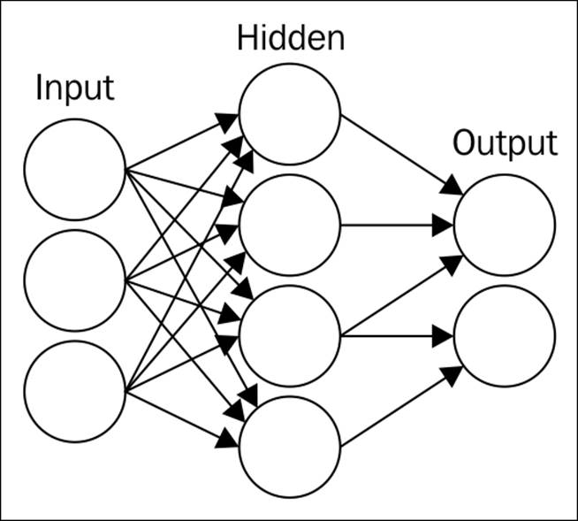
Figure 1
In the preceding graph, there are three layers—Input, Hidden and Output layer—which are the core of any neural network-based architecture. ANNs are a powerful technique used to solve many real-world problems such as classification, regression, and feature selection. ANNs have the ability to learn from new experiences in the form of new input data in order to improve the performance of classification- or regression-based tasks and to adapt themselves to changes in the input environment. Each circle in the preceding figure represents a neuron.
There are different variants of neural networks that are used in multiple different scenarios; we are going to explain a few of them conceptually in this chapter, and also their usage in practical applications:
· Single hidden layer neural network: This is the simplest form of neural network, as shown in the preceding figure. In it, there is only one hidden layer.
· Multiple hidden layer neural networks: In this form, more than one hidden layer will connect the input data to the output data. The complexity of calculation increases in this form as it requires more computational power in the system to process information.
· Feed forward neural networks: In this form of neural network architecture, the information passed is one-directional from one layer to another layer; there is no iteration from the first level of learning.
· Back propagation neural networks: In this form of neural network, there are two important steps. Feed forward works by passing information from the input to the hidden and from the hidden to the output layer; secondly, it calculates the error and propagates it back to the previous layers.
The feed-forward neural network model architecture is shown in the following figure, and backpropagation method is explained in Figure 3:
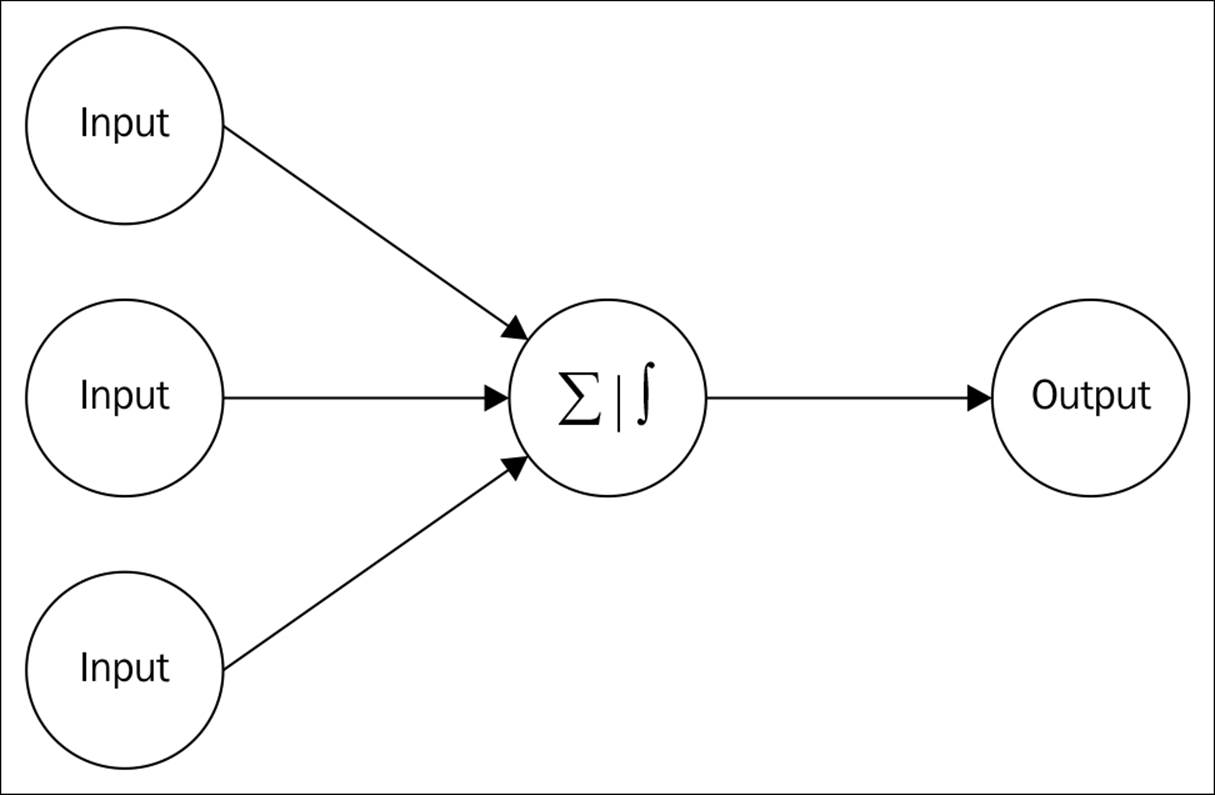
Figure 2
In the following figure, the red-colored arrows indicate information that has not passed through the output layer, and is again fed back to the input layer in terms of errors:
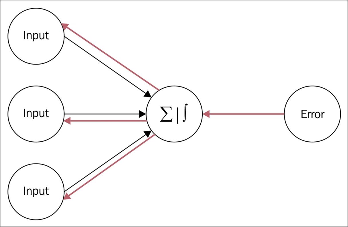
Figure 3
Having displayed the general architecture for different types of neural networks, let's visit the underlying math behind them.
Understanding the math behind the neural network
The neurons present in different layers--input, hidden, and output--are interconnected through a mathematical function called activation function, as displayed in Figure 1. There are different variants of the activation function, which are explained as follows. Understanding the activation function will help in implementation of the neural network model for better accuracy:
· Sigmoid function: This is frequently used by professionals in data mining and analytics, as it is easier to explain and implement too. The equation is mentioned here:
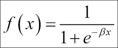
The sigmoid function, also known as the logistic function, is mostly used to transform the input data from the input layer to the mapping layer, or the hidden layer.
· Linear function: This is one of the simple functions typically used to transfer information from the de-mapping layer to the output layer. The formula is as follows:
f(x)=x
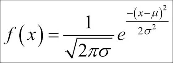
· Gaussian function: Gaussian functions are bell-shaped curves that are applicable for continuous variables, where the objective is to classify the output into multiple classes:
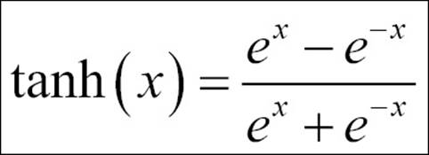
· Hyperbolic tangent function: This is another variant of transformation function; it is used to transform information from the mapping layer to the hidden layer:
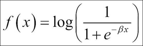
· Log sigmoid transfer function: The following formula explains the log sigmoid transfer function used in mapping the input layer to the hidden layer:
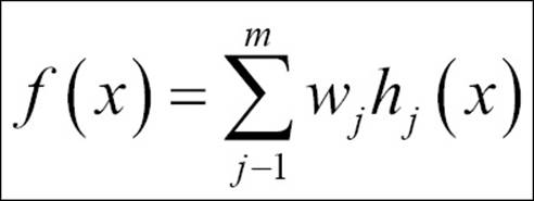
· Radial basis function: This is another activation function; it is used to transfer information from the de-mapping layer to the output layer:
Different types of transfer functions, as previously discussed, can be interchangeable in neural network architectures. They can be used in different stages such as input to hidden, hidden to output, and so on, to improve the model accuracy.
Neural network implementation in R
R programming for statistical computing provides three different libraries to perform the neural network model for various tasks. These three are nnet, neuralnet, and rsnns. In this chapter, we will use ArtPiece_1.csv and two libraries, nnet and neuralnet, to perform various tasks. The syntax for neural networks in those two libraries can be explained as follows.
The neuralnet library depends on two other libraries, grid and mass; while installing the neuralnet library, you have to make sure that these two dependency libraries are installed properly. In fitting a neural network model, the desired level of accuracy in a model defines the required number of hidden layers with the number of neurons in it; the number of hidden layers increases as the level of complexity increases. This library provides an option for training of neural networks using backpropagation, resilient backpropagation with (Riedmiller, 1994) or without weight backtracking (Riedmiller and Braun, 1993), or the modified globally convergent version by Anastasiadis et al. (2005). The package allows flexible settings through custom choice of error and activation functions. Now let's look at the syntax and the components in it that dictate the accuracy of the model:
|
Formula |
To define the input and output relationship |
|
Data |
Dataset with the input and output variables. |
|
Hidden |
A vector specifying the number of hidden layers in it. For example, (10, 5, 2) means 10 hidden neurons in the first layer, 5 in the second, and 2 in the third layer. |
|
Stepmax |
Maximum number of steps to be used. |
|
Rep |
Number of iterations. |
|
Startweights |
Random weights for the connections. |
|
Algorithm |
The algorithm to be used to fit a neural network object.'backprop'-refers to backpropagation. The 'rprop+' and 'rprop-' refer to resilient backpropagation with and without weight backtracking respectively, while 'sag' and 'slr' refer to the smallest absolute gradient and smallest learning rate. |
|
Err.fct |
Two methods: sum squared error (SSE) for regression-based prediction and cross entropy (CE) for classification-based problems. |
|
Act.fct |
"logistic" and "tanh" are possible for the logistic function and tangent hyperbolicus. |
|
Linear.output |
If no activation function is applied to the output layer, it has to be TRUE. |
|
Likelihood |
If the error function is equal to the negative log-likelihood function, the information criteria AIC and BIC will be calculated. |
Table 1: neuralnet syntax description
Table 2 shows the syntax of the nnet library, which can also be used to create neural-network-based models:
|
Formula |
A formula defining the input-output relationship |
|
X |
A matrix or data frame containing the input variables. |
|
Y |
A matrix or data frame containing the output variables. |
|
Weights |
Weights. |
|
Size |
Number of units in the hidden layer. |
|
Data |
Dataset. |
|
Na.action |
If NAs found what should be taken. |
|
Entropy |
Switch for entropy (is equal to maximum conditional likelihood) fitting. Default by leastsquares. |
|
Softmax |
Switch for softmax (log-linear model) and maximum conditional likelihood fitting. Linout, Entropy, Softmax, and Censored are mutually exclusive. |
|
Decay |
Parameter for weight decay. |
|
Maxit |
Maximum number of iterations. |
|
Trace |
Switch for tracing optimization. |
Table 2: nnet syntax description
Having discussed the syntax in Table 1 for both the libraries, let's have a look at the dataset to be used for prediction and classification-based tasks:
> library(neuralnet)
Loading required package: grid
Loading required package: MASS
Warning message:
package 'neuralnet' was built under R version 3.2.3
The structure function for the dataset shows the types of variables and the size of the dataset we are going to use for this chapter:
> art<- read.csv("ArtPiece_1.csv")
> str(art)
'data.frame': 72983 obs. of 26 variables:
$ Cid : int 1 2 3 4 5 6 7 8 9 10 ...
$ Art.Auction.House : Factor w/ 3 levels "Artnet","Christie",..: 3 3 3 3 3 3 3 3 3 3 ...
$ IsGood.Purchase : int 0 0 0 0 0 0 0 0 0 0 ...
$ Critic.Ratings : num 8.9 9.36 7.38 6.56 6.94 ...
$ Buyer.No : int 21973 19638 19638 19638 19638 19638 19638 19638 21973 21973 ...
$ Zip.Code : int 33619 33619 33619 33619 33619 33619 33619 33619 33619 33619 ...
$ Art.Purchase.Date : Factor w/ 517 levels "1/10/2012","1/10/2013",..: 386 386 386 386 386 386 386 386 386 386 ...
$ Year.of.art.piece : Factor w/ 10 levels "01-01-1947","01-01-1948",..: 6 4 5 4 5 4 4 5 7 7 ...
$ Acq.Cost : num 49700 53200 34300 28700 28000 39200 29400 31500 39200 53900 ...
$ Art.Category : Factor w/ 33 levels "Abstract Art Type I",..: 1 13 13 13 30 24 31 30 31 30 ...
$ Art.Piece.Size : Factor w/ 864 levels "10in. X 10in.",..: 212 581 68 837 785 384 485 272 485 794 ...
$ Border.of.art.piece : Factor w/ 133 levels " ","Border 1",..: 2 40 48 48 56 64 74 85 74 97 ...
$ Art.Type : Factor w/ 1063 levels "Type 1","Type 10",..: 1 176 287 398 509 620 731 842 731 953 ...
$ Prominent.Color : Factor w/ 17 levels "Beige","Black",..: 14 16 8 15 15 16 2 16 2 14 ...
$ CurrentAuctionAveragePrice: int 52157 52192 28245 12908 22729 32963 20860 25991 44919 64169 ...
$ Brush : Factor w/ 4 levels "","Camel Hair Brush",..: 2 2 2 2 4 2 2 2 2 2 ...
$ Brush.Size : Factor w/ 5 levels "0","1","2","3",..: 2 2 3 2 3 3 3 3 3 2 ...
$ Brush.Finesse : Factor w/ 4 levels "Coarse","Fine",..: 2 2 1 2 1 1 1 1 1 2 ...
$ Art.Nationality : Factor w/ 5 levels "American","Asian",..: 3 1 1 1 1 3 3 1 3 1 ...
$ Top.3.artists : Factor w/ 5 levels "MF Hussain","NULL",..: 3 1 1 1 4 3 3 4 3 4 ...
$ CollectorsAverageprice : Factor w/ 13193 levels "#VALUE!","0",..: 11433 11808 7802 4776 7034 8536 7707 7355 9836 483 ...
$ GoodArt.check : Factor w/ 3 levels "NO","NULL","YES": 2 2 2 2 2 2 2 2 2 2 ...
$ AuctionHouseGuarantee : Factor w/ 3 levels "GREEN","NULL",..: 2 2 2 2 2 2 2 2 2 2 ...
$ Vnst : Factor w/ 37 levels "AL","AR","AZ",..: 6 6 6 6 6 6 6 6 6 6 ...
$ Is.It.Online.Sale : int 0 0 0 0 0 0 0 0 0 0 ...
$ Min.Guarantee.Cost : int 7791 7371 9723 4410 7140 4158 3731 5775 3374 11431 ...
Neural networks for prediction
The use of neural networks for prediction requires the dependent/target/output variable to be numeric, and all the input/independent/feature variables can be of any type. From the ArtPiece dataset, we are going to predict what is going to be the current auction average price based on all the parameters available. Before applying a neural-network-based model, it is important to preprocess the data, by excluding the missing values and any transformation if required; hence, let's preprocess the data:
library(neuralnet)
art<- read.csv("ArtPiece_1.csv")
str(art)
#data conversion for categorical features
art$Art.Auction.House<-as.factor(art$Art.Auction.House)
art$IsGood.Purchase<-as.factor(art$IsGood.Purchase)
art$Art.Category<-as.factor(art$Art.Category)
art$Prominent.Color<-as.factor(art$Prominent.Color)
art$Brush<-as.factor(art$Brush)
art$Brush.Size<-as.factor(art$Brush.Size)
art$Brush.Finesse<-as.factor(art$Brush.Finesse)
art$Art.Nationality<-as.factor(art$Art.Nationality)
art$Top.3.artists<-as.factor(art$Top.3.artists)
art$GoodArt.check<-as.factor(art$GoodArt.check)
art$AuctionHouseGuarantee<-as.factor(art$AuctionHouseGuarantee)
art$Is.It.Online.Sale<-as.factor(art$Is.It.Online.Sale)
#data conversion for numeric features
art$Critic.Ratings<-as.numeric(art$Critic.Ratings)
art$Acq.Cost<-as.numeric(art$Acq.Cost)
art$CurrentAuctionAveragePrice<-as.numeric(art$CurrentAuctionAveragePrice)
art$CollectorsAverageprice<-as.numeric(art$CollectorsAverageprice)
art$Min.Guarantee.Cost<-as.numeric(art$Min.Guarantee.Cost)
#removing NA, Missing values from the data
fun1<-function(x){
ifelse(x=="#VALUE!",NA,x)
}
art<-as.data.frame(apply(art,2,fun1))
art<-na.omit(art)
#keeping only relevant variables for prediction
art<-art[,c("Art.Auction.House","IsGood.Purchase","Art.Category",
"Prominent.Color","Brush","Brush.Size","Brush.Finesse",
"Art.Nationality","Top.3.artists","GoodArt.check",
"AuctionHouseGuarantee","Is.It.Online.Sale","Critic.Ratings",
"Acq.Cost","CurrentAuctionAveragePrice","CollectorsAverageprice",
"Min.Guarantee.Cost")]
#creating dummy variables for the categorical variables
library(dummy)
art_dummy<-dummy(art[,c("Art.Auction.House","IsGood.Purchase","Art.Category",
"Prominent.Color","Brush","Brush.Size","Brush.Finesse",
"Art.Nationality","Top.3.artists","GoodArt.check",
"AuctionHouseGuarantee","Is.It.Online.Sale")],int=F)
art_num<-art[,c("Critic.Ratings",
"Acq.Cost","CurrentAuctionAveragePrice","CollectorsAverageprice",
"Min.Guarantee.Cost")]
art<-cbind(art_num,art_dummy)
## 70% of the sample size
smp_size <- floor(0.70 * nrow(art))
## set the seed to make your partition reproductible
set.seed(123)
train_ind <- sample(seq_len(nrow(art)), size = smp_size)
train <- art[train_ind, ]
test <- art[-train_ind, ]
fun2<-function(x){
as.numeric(x)
}
train<-as.data.frame(apply(train,2,fun2))
test<-as.data.frame(apply(test,2,fun2))
In the training dataset, there are 50,867 observations and 17 variables, and in the test dataset, there are 21,801 observations and 17 variables. The current auction average price is the dependent variable for prediction, using only four other numeric variables as features:
>fit<- neuralnet(formula = CurrentAuctionAveragePrice ~ Critic.Ratings + Acq.Cost + CollectorsAverageprice + Min.Guarantee.Cost, data = train, hidden = 15, err.fct = "sse", linear.output = F)
> fit
Call: neuralnet(formula = CurrentAuctionAveragePrice ~ Critic.Ratings + Acq.Cost + CollectorsAverageprice + Min.Guarantee.Cost, data = train, hidden = 15, err.fct = "sse", linear.output = F)
1 repetition was calculated.
Error Reached Threshold Steps
1 54179625353167 0.004727494957 23
A summary of the main results of the model is provided by result.matrix. A snapshot of the result.matrix is given as follows:
> fit$result.matrix
1
error 54179625353167.000000000000
reached.threshold 0.004727494957
steps 23.000000000000
Intercept.to.1layhid1 -0.100084491816
Critic.Ratings.to.1layhid1 0.686332945444
Acq.Cost.to.1layhid1 0.196864454378
CollectorsAverageprice.to.1layhid1 -0.793174429352
Min.Guarantee.Cost.to.1layhid1 0.528046199494
Intercept.to.1layhid2 0.973616842194
Critic.Ratings.to.1layhid2 0.839826678316
Acq.Cost.to.1layhid2 0.077798897157
CollectorsAverageprice.to.1layhid2 0.988149246218
Min.Guarantee.Cost.to.1layhid2 -0.385031389636
Intercept.to.1layhid3 -0.008367359937
Critic.Ratings.to.1layhid3 -1.409715725621
Acq.Cost.to.1layhid3 -0.384200569485
CollectorsAverageprice.to.1layhid3 -1.019243809714
Min.Guarantee.Cost.to.1layhid3 0.699876747202
Intercept.to.1layhid4 2.085203047278
Critic.Ratings.to.1layhid4 0.406934874266
Acq.Cost.to.1layhid4 1.121189503896
CollectorsAverageprice.to.1layhid4 1.405748076570
Min.Guarantee.Cost.to.1layhid4 -1.043884892202
Intercept.to.1layhid5 0.862634752109
Critic.Ratings.to.1layhid5 0.814364667751
Acq.Cost.to.1layhid5 0.502879862694
If the error function is equal to the negative log likelihood function, the error refers to the likelihood as it is used to calculate the Akaike Information Criterion (AIC). We can store the covariate and response data in a matrix:
> output<-cbind(fit$covariate,fit$result.matrix[[1]])
> head(output)
[,1] [,2] [,3] [,4] [,5]
[1,] 14953 49000 10727 5775 54179625353167
[2,] 35735 38850 9494 12418 54179625353167
[3,] 34751 43750 8738 9611 54179625353167
[4,] 31599 41615 5955 4158 54179625353167
[5,] 10437 34755 8390 4697 54179625353167
[6,] 13177 54670 13024 11921 54179625353167
To compare the results of a neural network model, we can use different tuning factors such as changing the algorithm, hidden layer, and learning rate. As an example, only four numeric features were used to generate the prediction; we could have used all the 91 features for prediction of the current auction average price variable. We can also use a different algorithm from the nnet library, as follows:
> fit<-nnet(CurrentAuctionAveragePrice~Critic.Ratings+Acq.Cost+
+ CollectorsAverageprice+Min.Guarantee.Cost,data=train,
+ size=100)
# weights: 601
initial value 108359809492660.125000
final value 108359250706334.000000
converged
> fit
a 4-100-1 network with 601 weights
inputs: Critic.Ratings Acq.Cost CollectorsAverageprice Min.Guarantee.Cost
output(s): CurrentAuctionAveragePrice
options were -
Both the libraries provide equal results; there is no difference in the model result, but to tune the results further, it is important to look at the model tuning parameters such as learning rate, hidden neurons, and so on. The following graph shows the neural network architecture:
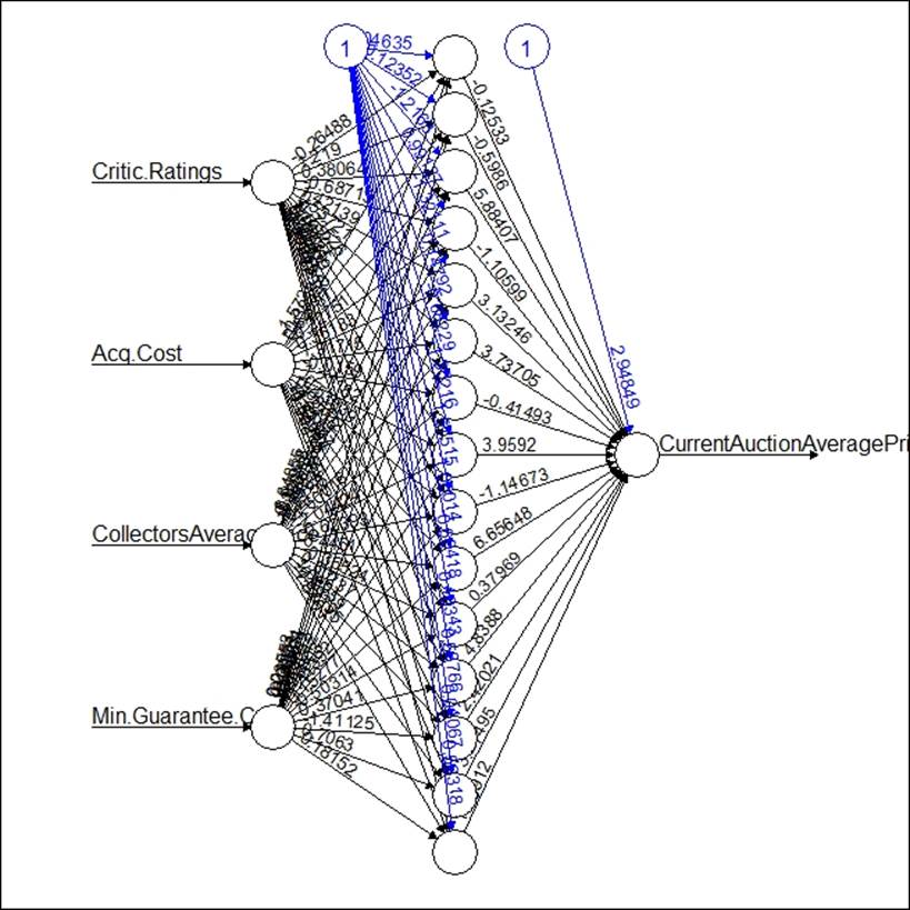
The model for predicting the unseen data points can be implemented using the compute function available in the neuralnet library, and the predict function available in the nnet library.
Neural networks for classification
For classification-based projects, the dependent variable can be binary or can have multiple levels, such as credit card fraud detection, classification of customers into different clusters as far as the marketing is concerned, and so on. In the current scenario from the ArtPiece dataset, we are trying to predict whether a work of art is a good purchase, or not, by taking a few business-relevant variables. For demo purposes, we have considered only a few features, but other features present in the dataset can be used to generate a better result:
> fit<-neuralnet(IsGood.Purchase_1~Brush.Size_1+Brush.Size_2+Brush.Size_3+
+ Brush.Finesse_Coarse+Brush.Finesse_Fine+
+ Art.Nationality_American+Art.Nationality_Asian+
+ Art.Nationality_European+GoodArt.check_YES,data=train[1:2000,],
+ hidden = 25,err.fct = "ce",linear.output = F)
> fit
Call: neuralnet(formula = IsGood.Purchase_1 ~ Brush.Size_1 + Brush.Size_2 + Brush.Size_3 + Brush.Finesse_Coarse + Brush.Finesse_Fine + Art.Nationality_American + Art.Nationality_Asian + Art.Nationality_European + GoodArt.check_YES, data = train[1:2000, ], hidden = 25, err.fct = "ce", linear.output = F)
1 repetition was calculated.
Error Reached Threshold Steps
1 666.1522488 0.009864324362 8254
> output<-cbind(fit$covariate,fit$result.matrix[[1]])
> head(output)
[,1] [,2] [,3] [,4] [,5] [,6] [,7] [,8] [,9] [,10]
[1,] 1 0 0 0 1 0 0 1 0 666.1522488
[2,] 1 0 0 0 1 1 0 0 0 666.1522488
[3,] 1 0 0 0 1 0 0 1 0 666.1522488
[4,] 0 1 0 1 0 0 0 1 0 666.1522488
[5,] 0 1 0 1 0 1 0 0 0 666.1522488
[6,] 1 0 0 0 1 1 0 0 0 666.1522488
The following graph shows the neural network model for classification:
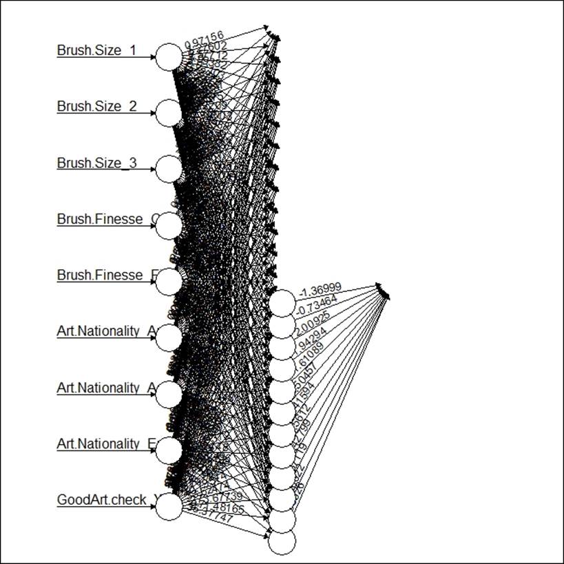
Using another library, nnet, for classification-based problems, the following result is derived:
> fit.nnet<-nnet(factor(IsGood.Purchase_1)~Brush.Size_1+Brush.Size_2+Brush.Size_3+
+ Brush.Finesse_Coarse+Brush.Finesse_Fine+
+ Art.Nationality_American+Art.Nationality_Asian+
+ Art.Nationality_European+GoodArt.check_YES,data=train[1:2000,],
+ size=9)
# weights: 100
initial value 872.587818
iter 10 value 684.034783
iter 20 value 667.751170
iter 30 value 667.027963
iter 40 value 666.337669
iter 50 value 666.156889
iter 60 value 666.138741
iter 70 value 666.137048
iter 80 value 666.136505
final value 666.136439
converged
> fit.nnet
a 9-9-1 network with 100 weights
inputs: Brush.Size_1 Brush.Size_2 Brush.Size_3 Brush.Finesse_Coarse Brush.Finesse_Fine Art.Nationality_American Art.Nationality_Asian Art.Nationality_European GoodArt.check_YES
output(s): factor(IsGood.Purchase_1)
options were - entropy fitting
Neural networks for forecasting
Neural networks can also be used to generate forecasts for a time series variable. There is a library called forecast in R that deploys feed-forward neural networks with a single hidden layer, and lagged inputs for forecasting univariate time series. For the forecasting example, we have taken an inbuilt dataset available in R called "Air Passengers" to apply the neural network.
The following table reflects the parameter arguments required by the nnetar function with the corresponding description of how they are being used in the model:
|
X |
Univariate time series with a time variable |
|
p |
Number of non-seasonal lags used as input |
|
P |
Number of seasonal lags used as input |
|
Size |
Number of nodes in the hidden layer |
|
Repeats |
Number of networks to fit with different random settings of weights |
|
Lambda |
This is known as box-cox transformation parameter |
|
Xreg |
External regressors used in fitting the model |
|
Mean |
Point forecasts as mean |
The actual time series looks as follows:
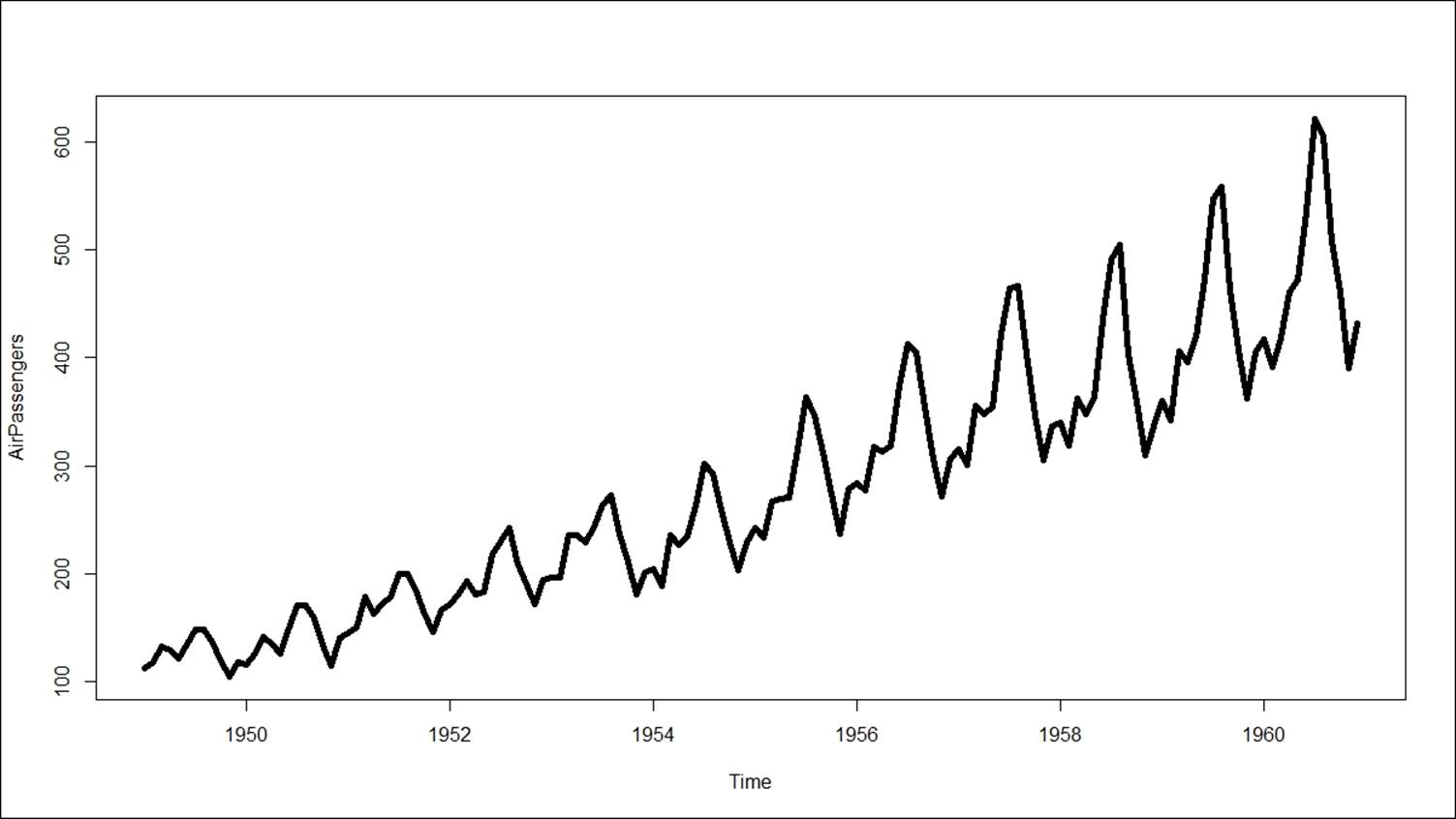
> fit<-nnetar(AirPassengers, p=9,P=,size = 10, repeats = 50,lambda = 0)
> plot(forecast(fit,10))
A neural-network-based forecasting model generates the following results as an output:
> summary(fit)
Length Class Mode
x 144 ts numeric
m 1 -none- numeric
p 1 -none- numeric
P 1 -none- numeric
scale 1 -none- numeric
size 1 -none- numeric
lambda 1 -none- numeric
model 50 nnetarmodels list
fitted 144 ts numeric
residuals 144 ts numeric
lags 10 -none- numeric
series 1 -none- character
method 1 -none- character
call 6 -none- call
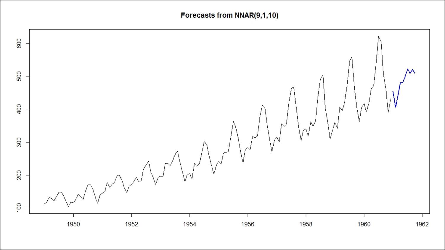
With a forecast of the next 10 periods, the graph looks as follows:
Merits and demerits of neural networks
The neural network method for performing classification, prediction, and forecasting is still recognized as a black box methodology in different industries. People still provide more importance to logistic regression than neural network because of its complexity in explaining the relationship between the dependent and independent variable.
The limitations of the neural network model can be stated as follows:
· In contrast to decision trees and rule extraction techniques, the knowledge (patterns) "discovered" by neural networks is not represented in a form understandable by humans.
· Knowledge in a trained neural network (NN) is encoded in its connection weights; hence, NN cannot be used for descriptive data mining (exploration).
· If NN are used for decision making, it is impossible to explain their decisions. Often other techniques have to be combined with NN for explanation.
Here are the merits of neural networks:
· Though it is a bit complex to understand and interpret the results, still it is considered a powerful technique for classification and regression
· It is considered a powerful machine learning technique for automatic predictive modeling
· It captures complex relationships in datasets, which a traditional algorithm such as linear regression or logistic regression fails to understand and interpret
References
Lichman, M. (2013). UCI Machine Learning Repository (http://archive.ics.uci.edu/ml). Irvine, CA: University of California, School of Information and Computer Science
Summary
In this chapter, we discussed various methods of performing classification, regression, and forecasting using the neural network model. Be it supervised or unsupervised data mining problems, neural-network-based implementations are popular not only among users but also among business stakeholders. We discussed which model to use where and the data requirement for each of the models. In this chapter, we specifically highlighted the importance of a powerful technique with better accuracy always for classification- and regression-based scenarios.
All materials on the site are licensed Creative Commons Attribution-Sharealike 3.0 Unported CC BY-SA 3.0 & GNU Free Documentation License (GFDL)
If you are the copyright holder of any material contained on our site and intend to remove it, please contact our site administrator for approval.
© 2016-2026 All site design rights belong to S.Y.A.