R Data Mining Blueprints (2016)
Chapter 8. Dimensionality Reduction
In this chapter, we are going to discuss about various methods to reduce data dimensions in performing analysis. In data mining, traditionally people used to apply principal component analysis (PCA) as a method to reduce the dimensionality in data. Though now in the age of big data, PCA is still valid, however along with that, many other techniques are being used to reduce dimensions. With the growth of data in volumes and variety, the dimension of data has been continuously on the rise. Dimensionality reduction techniques have many applications in different industries, such as in image processing, speech recognition, recommendation engines, text processing, and so on. The main problem in these application areas is not only high dimensional data but also high sparsity. Sparsity means that many columns in the dataset will have missing or blank values.
In this chapter, we will implement dimensionality reduction techniques such as PCA, singular value decomposition (SVD), and iterative feature selection method using a practical data set and R programming language.
In this chapter, we are going to discuss:
· Why dimensionality reduction is a business problem and what impact it may have on the predictive models
· What are the different techniques, with their respective positives and negatives, and data requirements and more
· Which technique to apply and in what situations, with little bit of mathematics behind the calculation
· An R programming based implementation and interpretation of results in a project
Why dimensionality reduction?
In various statistical analysis models, especially showing a cause and impact relationship between dependent variable and a set of independent variables, if the number of independent variables increases beyond a manageable stage (for example, 100 plus), then it is quite difficult to interpret each and every variable. For example, in weather forecast, nowadays low cost sensors are being deployed at various places and those sensors provide signals and data are being stored in the database. When 1000 plus sensors provide data, it is important to understand the pattern or at least which all sensors are meaningful in performing the desired task.
Another example, from a business standpoint, is that if more than 30 features are impacting a dependent variable (for example, Sales), as a business owner I cannot regulate all 30 factors and cannot form strategies for 30 dimensions. Of course, as a business owner I would be interested in looking at 3-4 dimensions that should explain 80% of the dependent variable in the data. From the preceding two examples, it is pretty clear that dimensionality is still a valid business problem. Apart from business and volume, there are other reasons such as computational cost, storage cost of data, and more, if a set of dimensions are not at all meaningful for the target variable or target function why would I store it in my database.
Dimensionality reduction is useful in big data mining applications in performing both supervised learning and unsupervised learning-based tasks, to:
· Identify the pattern how the variables work together
· Display the relationship in a low dimensional space
· Compress the data for further analysis so that redundant features can be removed
· Avoid overfitting as reduced feature set with reduced degrees of freedom does that
· Running algorithms on a reduced feature set would be much more faster than the base features
Two important aspects of data dimensionality are, first, variables that are highly correlated indicate high redundancy in the data, and the second, most important dimensions always have high variance. While working on dimension reduction, it is important to take note of these aspects and make necessary amendments to the process.
Hence, it is important to reduce the dimensions. Also, it is not a good idea to focus on many variables to control or regulate the target variable in a predictive model. In a multivariate study, the correlation between various independent variables affect the empirical likelihood function and affects the eigen values and eigen vectors through covariance matrix.
Techniques available for dimensionality reduction
The dimensionality reduction techniques can be classified into two major groups: parametric or model-based feature reduction and non-parametric feature reduction. In non-parametric feature reduction technique, the data dimension is reduced first and then the resulting data can be used to create any classification or predictive model, supervised or unsupervised. However, the parametric-based method emphasizes on monitoring the overall performance of a model and its accuracy by changing the features and hence deciding how many features are needed to represent the model. The following are the techniques generally used in data mining literature to reduce data dimensions:
· Non-parametric:
· PCA method
· Parametric method
· Forward feature selection
· Backward feature selection
We are going to discuss these methods in detail with the help of a dataset using R programming language. Apart from these techniques mentioned earlier, there are few more methods but not that popular, such as removing variables with low variance as they don't add much information to the target variable and also removing variables with many missing values. The latter comes under the missing value treatment method, but can still be used to reduce the features in a high dimensional dataset. There are two methods in R, prcomp() and princomp(), but they use two slightly different methods; princomp() uses eigen vectors and prcomp() uses SVD method. Some researchers favor prcomp() as a method over princomp() method. We are going to use two different methods here.
Which technique to apply where?
The usage of the technique actually depends upon the researcher; what he is looking at from the data. If you are looking at hidden features and want to represent the data in a low dimensional space, PCA is the method one should choose. If you are looking at building a good classification or prediction model, then it is not a good idea to perform PCA first; you should ideally include all the features and remove the redundant ones by any parametric method, such as forward or backward. Selection of techniques vary based on data availability, the problem statement, and the task that someone is planning to perform.
Principal component analysis
PCA is a multivariate statistical data analysis technique applicable for datasets with numeric variables only, which computes linear combinations of the original variables and those principal components are orthogonal to each other in the feature space. PCA is a method that uses eigen values and eigen vectors to compute the principal components, which is a linear combination of original variables. PCA can be used in regression modelling in order to remove the problem of multicollinearity in the dataset and can also be used in clustering exercise in order to understand unique group behaviors or segments existing in the dataset.
PCA assumes that the variables are linearly associated to form principal components and variables with high variance do not necessarily represent the best feature. The principal component analysis is based on a few theorems:
· The inverse of an orthogonal matrix is its transpose
· The original matrix times the transposed version of the original matrix are both symmetric
· A matrix is symmetric if it is an orthogonally diagonalizable matrix
· It uses variance matrix, not the correlation matrix to compute components
Following are the steps to perform principal component analysis:
1. Get a numerical dataset. If you have any categorical variable, remove it from the dataset so that mathematical computation can happen on the remaining variables.
2. In order to make the PCA work properly, data normalization should be done. This is done by deducting the mean of the column from each of the values for all the variables; ensure that the mean of the variables of the transformed data should be equal to 0.
We applied the following normalization formula:
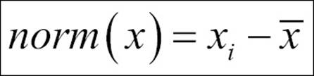
3. Calculate the covariance matrix on the reduced dataset. Covariance is a measure of two variables. A covariance matrix is a display of all the possible covariance values between all the different dimensions:
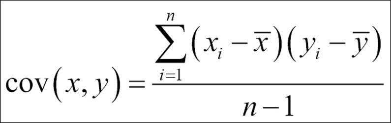
The sign of covariance is more important than its value; a positive covariance value indicates that both dimensions increase together and vice versa. Similarly, a negative value of covariance indicates that with an increase in one dimension, the other dimension decreases. If the covariance value is zero, it shows that the two dimensions are independent of each other and there is no relationship.
4. Calculate the eigen vectors and eigen values from the covariance matrix. All eigen vectors always come from a square matrix but all square matrix do not always generate an eigen vector. All eigen vectors of a matrix are orthogonal to each other.
5. Create a feature vector by taking eigen values in order from largest to smallest. The eigen vector with highest eigen value is the principal component of the dataset. From the covariance matrix, the eigen vectors are identified and the eigen values are ordered from largest to smallest:
Feature Vector = (Eigen1, Eigen2......Eigen 14)
6. Create low dimension data using the transposed version of the feature vector and transposed version of the normalized data. In order to get the transposed dataset, we are going to multiply the transposed feature vector and transposed normalized data.
Let's apply these steps in the following section.
Practical project around dimensionality reduction
We are going to apply dimensionality reduction procedure, both model-based approach and principal component-based approach, on the dataset to come up with less number of features so that we can use those features for classification of the customers into defaulters and no-defaulters.
For practical project, we have considered a dataset default of credit card clients.csv, which contains 30,000 samples and 24 attributes or dimensions. We are going to apply two different methods of feature reduction: the traditional way and the modern machine learning way.
Attribute description
The following are descriptions for the attributes from the dataset:
· X1: Amount of the given credit (NT dollar). It includes both the individual consumer credit and his/her family (supplementary) credit.
· X2: Gender (1 = male; 2 = female).
· X3: Education (1 = graduate school; 2 = university; 3 = high school; 4 = others).
· X4: Marital status (1 = married; 2 = single; 3 = others).
· X5: Age (year).
· X6 - X11: History of past payment. We tracked the past monthly payment records (from April to September, 2005) as follows:
· X6= the repayment status in September, 2005
· X7 = the repayment status in August, 2005; . . .
· X11 = the repayment status in April, 2005. The measurement scale for the repayment status is: -1 = pay duly; 1 = payment delay for one month; 2 = payment delay for two months; . . . 8 = payment delay for eight months; 9 = payment delay for nine months, and so on.
· X12-X17: Amount of bill statement (NT dollar).
· X12 = amount of bill statement in September, 2005;
· X13 = amount of bill statement in August, 2005; . . .
· X17 = amount of bill statement in April, 2005.
· X18-X23: Amount of previous payment (NT dollar).
· X18 = amount paid in September, 2005;
· X19 = amount paid in August, 2005; . . .
· X23 = amount paid in April, 2005.
Let's get the dataset and do the necessary normalization and transformation:
> setwd("select the working directory")
> default<-read.csv("default.csv")
corrplot::corrplot(cor(df),method="ellipse")
From the preceding correlations matrix, it is clear that there are some strong correlations between different variables from X12 to X17, which possibly can be clubbed together as linear combinations using PCA. The following graph shows the correlations between different variables:
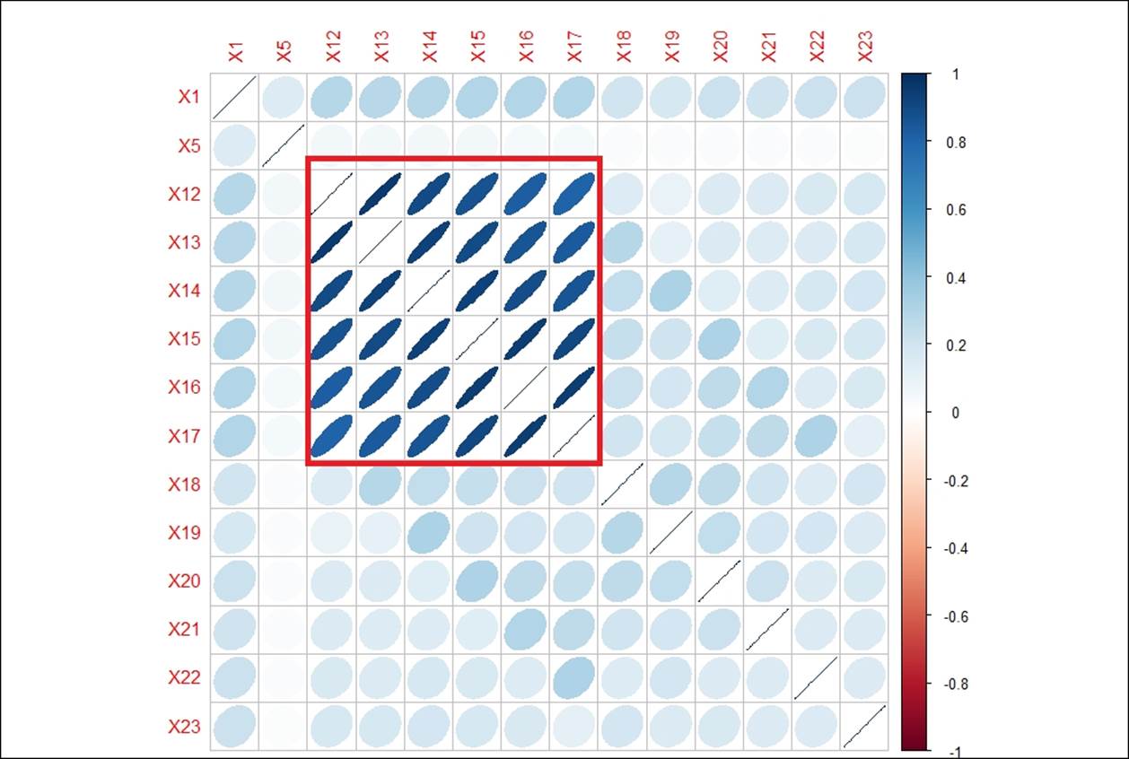
In the previous correlations graph, the strength of the correlation is reflected by the size of the ellipse and the color varying from red to blue. The blue ellipses indicate positive correlation and the white ones show no correlation. Variable X12 has a high degree of positive correlation with variables X13 to X17, with a correlation value of more than 80%.
Row number 1 contains the variable description and there are some columns which are categorical; we need to remove those from our dataset. Some other variables are shown as categorical and hence need to be converted back to numeric mode:
> df<-default[-1,-c(1,3:5,7:12,25)]
> func1<-function(x){
+ as.numeric(x)
+ }
> df<-as.data.frame(apply(df,2,func1))
> normalize-function(x){
+ (x-mean(x))
+ }
Using func1, we convert the non-numeric variables into numeric so that we can apply the normalization function (normalize), which is doing data normalization. After applying normalization, the dataset will look like the one as shown next. To apply principal component analysis, either we can use mean normalized dataset as an input or we can use the base dataset with correlations or a covariance matrix as an input. If we are not going to normalize the dataset, the variable with the highest variance will become the first principal component and hence will dominate other relevant principal components:
> dn<-as.data.frame(apply(df,2,normalize))
> str(dn)
'data.frame': 30000 obs. of 14 variables:
$ X1 : num -147484 -47484 -77484 -117484 -117484 ...
$ X5 : num -11.49 -9.49 -1.49 1.51 21.51 ...
$ X12: num -47310 -48541 -21984 -4233 -42606 ...
$ X13: num -46077 -47454 -35152 -946 -43509 ...
$ X14: num -46324 -44331 -33454 2278 -11178 ...
$ X15: num -43263 -39991 -28932 -14949 -22323 ...
$ X16: num -40311 -36856 -25363 -11352 -21165 ...
$ X17: num -38872 -35611 -23323 -9325 -19741 ...
$ X18: num -5664 -5664 -4146 -3664 -3664 ...
$ X19: num -5232 -4921 -4421 -3902 30760 ...
$ X20: num -5226 -4226 -4226 -4026 4774 ...
$ X21: num -4826 -3826 -3826 -3726 4174 ...
$ X22: num -4799 -4799 -3799 -3730 -4110 ...
$ X23: num -5216 -3216 -216 -4216 -4537 ...
Running principal component analysis:
> options(digits = 2)
> pca1<-princomp(df,scores = T, cor = T)
> summary(pca1)
Importance of components:
Comp.1 Comp.2 Comp.3 Comp.4 Comp.5 Comp.6 Comp.7 Comp.8 Comp.9 Comp.10 Comp.11
Standard deviation 2.43 1.31 1.022 0.962 0.940 0.934 0.883 0.852 0.841 0.514 0.2665
Proportion of Variance 0.42 0.12 0.075 0.066 0.063 0.062 0.056 0.052 0.051 0.019 0.0051
Cumulative Proportion 0.42 0.55 0.620 0.686 0.749 0.812 0.867 0.919 0.970 0.989 0.9936
Comp.12 Comp.13 Comp.14
Standard deviation 0.2026 0.1592 0.1525
Proportion of Variance 0.0029 0.0018 0.0017
Cumulative Proportion 0.9965 0.9983 1.0000
Principal component (PC) 1 explains 42% variation in the dataset and principal component 2 explains 12% variation in the dataset. This means that first PC has closeness to 42% of the total data points in the n-dimensional space. From the preceding results, it is clear that the first 8 principal components capture 91.9% variation in the dataset. Rest 8% variation in the dataset is explained by 6 other principal components. Now the question is how many principal components should be chosen. The general rule of thumb is 80-20, if 80% variation in the data can be explained by 20% of the principal components. There are 14 variables; we have to look at how many components explain 80% variation in the dataset cumulatively. Hence, it is recommended, based on the 80:20 Pareto principle, taking 6 principal components which explain 81% variation cumulatively.
In a multivariate dataset, the correlation between the component and the original variables is called the component loading. The loadings of the principal components are as follows:
> #Loadings of Principal Components
> pca1$loadings
Loadings:
Comp.1 Comp.2 Comp.3 Comp.4 Comp.5 Comp.6 Comp.7 Comp.8 Comp.9 Comp.10 Comp.11 Comp.12 Comp.13 Comp.14
X1 -0.165 0.301 0.379 0.200 0.111 0.822
X5 0.870 -0.338 -0.331
X12 -0.372 -0.191 0.567 0.416 0.433 0.184 -0.316
X13 -0.383 -0.175 0.136 0.387 -0.345 -0.330 0.645
X14 -0.388 -0.127 -0.114 -0.121 0.123 -0.485 -0.496 -0.528
X15 -0.392 -0.120 0.126 -0.205 -0.523 0.490 0.362 0.346
X16 -0.388 -0.106 0.107 -0.420 0.250 -0.718 -0.227
X17 -0.381 0.165 -0.489 0.513 -0.339 0.428
X18 -0.135 0.383 -0.173 -0.362 -0.226 -0.201 0.749
X19 -0.117 0.408 -0.201 -0.346 -0.150 0.407 -0.280 -0.578 0.110 0.147 0.125
X20 -0.128 0.392 -0.122 -0.245 0.239 -0.108 0.785 -0.153 0.145 -0.125
X21 -0.117 0.349 0.579 -0.499 -0.462 0.124 -0.116
X22 -0.114 0.304 0.609 0.193 0.604 0.164 -0.253
X23 -0.106 0.323 0.367 -0.658 -0.411 -0.181 -0.316
Comp.1 Comp.2 Comp.3 Comp.4 Comp.5 Comp.6 Comp.7 Comp.8 Comp.9 Comp.10 Comp.11 Comp.12 Comp.13 Comp.14
SS loadings 1.000 1.000 1.000 1.000 1.000 1.000 1.000 1.000 1.000 1.000 1.000 1.000 1.000 1.000
Proportion Var 0.071 0.071 0.071 0.071 0.071 0.071 0.071 0.071 0.071 0.071 0.071 0.071 0.071 0.071
Cumulative Var 0.071 0.143 0.214 0.286 0.357 0.429 0.500 0.571 0.643 0.714 0.786 0.857 0.929 1.000
> pca1
Call:
princomp(x = df, cor = T, scores = T)
Standard deviations:
Comp.1 Comp.2 Comp.3 Comp.4 Comp.5 Comp.6 Comp.7 Comp.8 Comp.9 Comp.10
2.43 1.31 1.02 0.96 0.94 0.93 0.88 0.85 0.84 0.51
Comp.11 Comp.12 Comp.13 Comp.14
0.27 0.20 0.16 0.15
14 variables and 30000 observations.
The following graph indicates the percentage variance explained by the principal components:
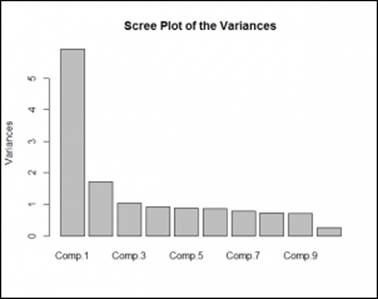
Following scree plot shows how many principal components we should retain for the dataset:
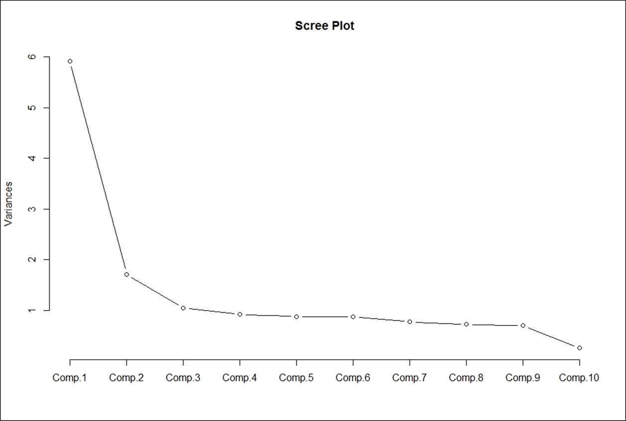
From the preceding scree plot, it is concluded that the first principal component has the highest variance, then second and third respectively. From the graph, three principal components have higher variance than the other principal components.
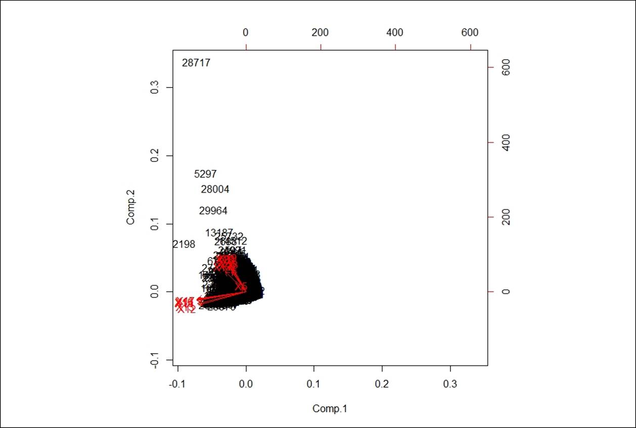
Following biplot indicates the existence of principal components in a n-dimensional space:
The diagonal elements of the covariance matrix are the variances of the variables; the off-diagonal variables are covariance between different variables:
> diag(cov(df))
X1 X5 X12 X13 X14 X15 X16 X17 X18 X19 X20
1.7e+10 8.5e+01 5.4e+09 5.1e+09 4.8e+09 4.1e+09 3.7e+09 3.5e+09 2.7e+08 5.3e+08 3.1e+08
X21 X22 X23
2.5e+08 2.3e+08 3.2e+08
The interpretation of scores is little bit tricky because they do not have any meaning until and unless you use them to plot on a straight line as defined by the eigen vector. PC scores are the co-ordinates of each point with respect to the principal axis. Using eigen values you can extract eigen vectors which describe a straight line to explain the PCs. The PCA is a form of multidimensional scaling as it represents data in a lower dimension without losing much information about the variables. The component scores are basically the linear combination of loading times the mean centred scaled dataset.
When we deal with multivariate data, it is really difficult to visualize and build models around it. In order to reduce the features, PCA is used; it reduces the dimensions so that we can plot, visualize, and predict the future, in a lower dimension. The principal components are orthogonal to each other, which means that they are uncorrelated. At the data pre-processing stage, the scaling function decides what type of input data matrix is required. If the mean centring approach is used as transformation then covariance matrix should be used as input data for PCA. If a scaling function does a standard z-score transformation, assuming standard deviation is equal to 1, then correlation matrix should be used as input data.
Now the question is where to apply which transformation. If the variables are highly skewed then z-score transformation and PCA based on correlation should be used. If the input data is approximately symmetric then mean centring approach and PCA based on covariance should be applied.
Now, let's look at the principal component scores:
> #scores of the components
> pca1$scores[1:10,]
Comp.1 Comp.2 Comp.3 Comp.4 Comp.5 Comp.6 Comp.7 Comp.8 Comp.9 Comp.10 Comp.11 Comp.12 Comp.13 Comp.14
[1,] 1.96 -0.54 -1.330 0.1758 -0.0175 0.0029 0.013 -0.057 -0.22 0.020 0.0169 0.0032 -0.0082 0.00985
[2,] 1.74 -0.22 -0.864 0.2806 -0.0486 -0.1177 0.099 -0.075 0.29 -0.073 -0.0055 -0.0122 0.0040 0.00072
[3,] 1.22 -0.28 -0.213 0.0082 -0.1269 -0.0627 -0.014 -0.084 -0.28 -0.016 0.1125 0.0805 0.0413 -0.05711
[4,] 0.54 -0.67 -0.097 -0.2924 -0.0097 0.1086 -0.134 -0.063 -0.60 0.144 0.0017 -0.1381 -0.0183 -0.05794
[5,] 0.85 0.74 1.392 -1.6589 0.3178 0.5846 -0.543 -1.113 -1.24 -0.038 -0.0195 -0.0560 0.0370 -0.01208
[6,] 0.54 -0.71 -0.081 -0.2880 -0.0924 0.1145 -0.194 -0.015 -0.58 0.505 0.0276 -0.1848 -0.0114 -0.14273
[7,] -15.88 -0.96 -1.371 -1.1334 0.3062 0.0641 0.514 0.771 0.99 -2.890 -0.4219 0.4631 0.3738 0.32748
[8,] 1.80 -0.29 -1.182 0.4394 -0.0620 -0.0440 0.076 -0.013 0.26 0.046 0.0484 0.0584 0.0268 -0.04504
[9,] 1.41 -0.21 -0.648 0.1902 -0.0653 -0.0658 0.040 0.122 0.33 -0.028 -0.0818 0.0296 -0.0605 0.00106
[10,] 1.69 -0.18 -0.347 -0.0891 0.5969 -0.2973 -0.453 -0.140 -0.74 -0.137 0.0248 -0.0218 0.0028 0.00423
Larger eigen values indicate larger variation in a dimension. The following script shows how to compute eigen values and eigen vectors from the correlation matrix:
> eigen(cor(df),TRUE)$values
[1] 5.919 1.716 1.045 0.925 0.884 0.873 0.780 0.727 0.707 0.264 0.071 0.041 0.025 0.023
head(eigen(cor(df),TRUE)$vectors)
[,1] [,2] [,3] [,4] [,5] [,6] [,7] [,8] [,9] [,10] [,11] [,12] [,13]
[1,] -0.165 0.301 0.379 0.2004 -0.035 -0.078 0.1114 0.0457 0.822 -0.0291 -0.00617 -0.0157 0.00048
[2,] -0.033 0.072 0.870 -0.3385 0.039 0.071 -0.0788 -0.0276 -0.331 -0.0091 0.00012 0.0013 -0.00015
[3,] -0.372 -0.191 0.034 0.0640 -0.041 -0.044 0.0081 -0.0094 -0.010 0.5667 0.41602 0.4331 0.18368
[4,] -0.383 -0.175 0.002 -0.0075 -0.083 -0.029 -0.0323 0.1357 -0.017 0.3868 0.03836 -0.3452 -0.32953
[5,] -0.388 -0.127 -0.035 -0.0606 -0.114 0.099 -0.1213 -0.0929 0.019 0.1228 -0.48469 -0.4957 0.08662
[6,] -0.392 -0.120 -0.034 -0.0748 -0.029 0.014 0.1264 -0.0392 -0.019 -0.2052 -0.52323 0.4896 0.36210
[,14]
[1,] 0.0033
[2,] 0.0011
[3,] -0.3164
[4,] 0.6452
[5,] -0.5277
[6,] 0.3462
The standard deviation of the individual principal components and the mean of all the principal components is as follows:
> pca1$sdev
Comp.1 Comp.2 Comp.3 Comp.4 Comp.5 Comp.6 Comp.7 Comp.8 Comp.9 Comp.10 Comp.11 Comp.12 Comp.13 Comp.14
2.43 1.31 1.02 0.96 0.94 0.93 0.88 0.85 0.84 0.51 0.27 0.20 0.16 0.15
> pca1$center
X1 X5 X12 X13 X14 X15 X16 X17 X18 X19 X20 X21 X22 X23
-9.1e-12 -1.8e-15 -6.8e-13 -3.0e-12 4.2e-12 4.1e-12 -1.4e-12 5.1e-13 7.0e-14 4.4e-13 2.9e-13 2.7e-13 -2.8e-13 -3.9e-13
Using the normalized data, and with no correlations table as an input, the following result is obtained. There is no difference in the output as we got the pca2 model in comparison to pca1:
> pca2<-princomp(dn)
> summary(pca2)
Importance of components:
Comp.1 Comp.2 Comp.3 Comp.4 Comp.5 Comp.6 Comp.7 Comp.8 Comp.9 Comp.10 Comp.11 Comp.12 Comp.13 Comp.14
Standard deviation 1.7e+05 1.2e+05 3.7e+04 2.8e+04 2.1e+04 2.0e+04 1.9e+04 1.7e+04 1.6e+04 1.2e+04 1.0e+04 8.8e+03 8.2e+03 9.1e+00
Proportion of Variance 6.1e-01 3.0e-01 3.1e-02 1.7e-02 9.4e-03 9.0e-03 7.5e-03 6.4e-03 5.8e-03 3.0e-03 2.4e-03 1.7e-03 1.5e-03 1.8e-09
Cumulative Proportion 6.1e-01 9.1e-01 9.4e-01 9.5e-01 9.6e-01 9.7e-01 9.8e-01 9.9e-01 9.9e-01 9.9e-01 1.0e+00 1.0e+00 1.0e+00 1.0e+00
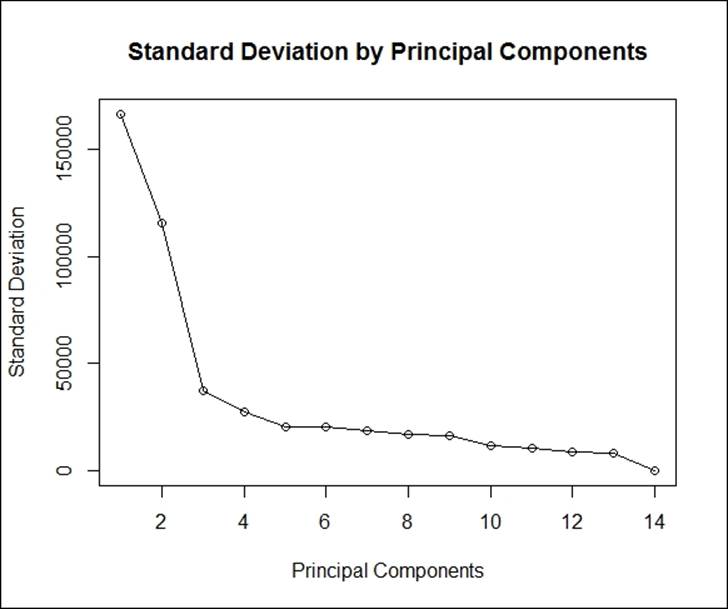
The next screen plot indicates that three principal components constitute most of the variation in the dataset. The x axis shows the principal components and the y axis shows the standard deviation (variance = square of the standard deviation).
The following script shows the plot being created:
> result<-round(summary(pca2)[1]$sdev,0)
> #scree plot
> plot(result, main = "Standard Deviation by Principal Components",
+ xlab="Principal Components",ylab="Standard Deviation",type='o')
Using the prcomp() function, which uses the SVD method to perform dimensionality reduction can be analysed as follows. prcomp() method accepts raw dataset as input and it has a built in argument which requires to make the scaling as true:
> pca<-prcomp(df,scale. = T)
> summary(pca)
Importance of components:
PC1 PC2 PC3 PC4 PC5 PC6 PC7 PC8 PC9 PC10
Standard deviation 2.433 1.310 1.0223 0.9617 0.9400 0.9342 0.8829 0.8524 0.8409 0.5142
Proportion of Variance 0.423 0.123 0.0746 0.0661 0.0631 0.0623 0.0557 0.0519 0.0505 0.0189
Cumulative Proportion 0.423 0.545 0.6200 0.6861 0.7492 0.8115 0.8672 0.9191 0.9696 0.9885
PC11 PC12 PC13 PC14
Standard deviation 0.26648 0.20263 0.15920 0.15245
Proportion of Variance 0.00507 0.00293 0.00181 0.00166
Cumulative Proportion 0.99360 0.99653 0.99834 1.00000
From the result we can see that there is little variation in the two methods. The SVD approach also shows that the first 8 components explain 91.91% variation in the dataset. From the documentation of prcomp and princomp, there is no difference in the type of PCA, but there is a difference in the method used to calculate PCA. The two methods are spectral decomposition and singular decomposition.
In spectral decomposition, as shown in the princomp function, the calculation is done using eigen on the correlation or covariance matrix. Using the prcomp method, the calculation is done by the SVD method.
To get the rotation matrix, which is equivalent to the loadings matrix in the princomp() method, we can use the following script:
> summary(pca)$rotation
PC1 PC2 PC3 PC4 PC5 PC6 PC7 PC8 PC9 PC10 PC11
X1 0.165 0.301 -0.379 0.2004 -0.035 0.078 -0.1114 -0.04567 0.822 -0.0291 0.00617
X5 0.033 0.072 -0.870 -0.3385 0.039 -0.071 0.0788 0.02765 -0.331 -0.0091 -0.00012
X12 0.372 -0.191 -0.034 0.0640 -0.041 0.044 -0.0081 0.00937 -0.010 0.5667 -0.41602
X13 0.383 -0.175 -0.002 -0.0075 -0.083 0.029 0.0323 -0.13573 -0.017 0.3868 -0.03836
X14 0.388 -0.127 0.035 -0.0606 -0.114 -0.099 0.1213 0.09293 0.019 0.1228 0.48469
X15 0.392 -0.120 0.034 -0.0748 -0.029 -0.014 -0.1264 0.03915 -0.019 -0.2052 0.52323
X16 0.388 -0.106 0.034 -0.0396 0.107 0.099 0.0076 0.04964 -0.024 -0.4200 -0.06824
X17 0.381 -0.094 0.018 0.0703 0.165 -0.070 -0.0079 -0.00015 -0.059 -0.4888 -0.51341
X18 0.135 0.383 0.173 -0.3618 -0.226 -0.040 0.2010 -0.74901 -0.020 -0.0566 -0.04763
X19 0.117 0.408 0.201 -0.3464 -0.150 -0.407 0.2796 0.57842 0.110 0.0508 -0.14725
X20 0.128 0.392 0.122 -0.2450 0.239 0.108 -0.7852 0.06884 -0.153 0.1449 -0.00015
X21 0.117 0.349 0.062 0.0946 0.579 0.499 0.4621 0.07712 -0.099 0.1241 0.11581
X22 0.114 0.304 -0.060 0.6088 0.193 -0.604 -0.0143 -0.16435 -0.253 0.0601 0.09944
X23 0.106 0.323 -0.050 0.3672 -0.658 0.411 -0.0253 0.18089 -0.316 -0.0992 -0.03495
PC12 PC13 PC14
X1 -0.0157 0.00048 -0.0033
X5 0.0013 -0.00015 -0.0011
X12 0.4331 0.18368 0.3164
X13 -0.3452 -0.32953 -0.6452
X14 -0.4957 0.08662 0.5277
X15 0.4896 0.36210 -0.3462
X16 0.2495 -0.71838 0.2267
X17 -0.3386 0.42770 -0.0723
X18 0.0693 0.04488 0.0846
X19 0.0688 -0.03897 -0.1249
X20 -0.1247 -0.02541 0.0631
X21 -0.0010 0.08073 -0.0423
X22 0.0694 -0.09520 0.0085
X23 -0.0277 0.01719 -0.0083
The rotated dataset can be retrieved by using argument x from the summary result of the prcomp() method:
> head(summary(pca)$x)
PC1 PC2 PC3 PC4 PC5 PC6 PC7 PC8 PC9 PC10 PC11 PC12
[1,] -1.96 -0.54 1.330 0.1758 -0.0175 -0.0029 -0.013 0.057 -0.22 0.020 -0.0169 0.0032
[2,] -1.74 -0.22 0.864 0.2806 -0.0486 0.1177 -0.099 0.075 0.29 -0.073 0.0055 -0.0122
[3,] -1.22 -0.28 0.213 0.0082 -0.1269 0.0627 0.014 0.084 -0.28 -0.016 -0.1125 0.0805
[4,] -0.54 -0.67 0.097 -0.2924 -0.0097 -0.1086 0.134 0.063 -0.60 0.144 -0.0017 -0.1381
[5,] -0.85 0.74 -1.392 -1.6588 0.3178 -0.5846 0.543 1.113 -1.24 -0.038 0.0195 -0.0560
[6,] -0.54 -0.71 0.081 -0.2880 -0.0924 -0.1145 0.194 0.015 -0.58 0.505 -0.0276 -0.1848
PC13 PC14
[1,] -0.0082 -0.00985
[2,] 0.0040 -0.00072
[3,] 0.0413 0.05711
[4,] -0.0183 0.05794
[5,] 0.0370 0.01208
[6,] -0.0114 0.14273
> biplot(prcomp(df,scale. = T))
The orthogonal red lines indicate the principal components that explain the entire dataset.
Having discussed various methods of variable reduction, what is going to be the output; the output should be a new dataset, in which all the principal components will be uncorrelated with each other. This dataset can be used for any task such as classification, regression, or clustering, among others. From the results of the principal component analysis how we get the new dataset; let's have a look at the following script:
> #calculating Eigen vectors
> eig<-eigen(cor(df))
> #Compute the new dataset
> eigvec<-t(eig$vectors) #transpose the eigen vectors
> df_scaled<-t(dn) #transpose the adjusted data
> df_new<-eigvec %*% df_scaled
> df_new<-t(df_new)
> colnames(df_new)<-c("PC1","PC2","PC3","PC4",
+ "PC5","PC6","PC7","PC8",
+ "PC9","PC10","PC11","PC12",
+ "PC13","PC14")
> head(df_new)
PC1 PC2 PC3 PC4 PC5 PC6 PC7 PC8 PC9 PC10 PC11 PC12
[1,] 128773 -19470 -49984 -27479 7224 10905 -14647 -4881 -113084 -2291 1655 2337
[2,] 108081 11293 -12670 -7308 3959 2002 -3016 -1662 -32002 -9819 -295 920
[3,] 80050 -7979 -24607 -11803 2385 3411 -6805 -3154 -59324 -1202 7596 7501
[4,] 37080 -39164 -41935 -23539 2095 9931 -15015 -4291 -92461 12488 -11 -7943
[5,] 77548 356 -50654 -38425 7801 20782 -19707 -28953 -88730 -12624 -9028 -4467
[6,] 34793 -42350 -40802 -22729 -2772 9948 -17731 -2654 -91543 37090 2685 -10960
PC13 PC14
[1,] -862 501
[2,] -238 -97
[3,] 2522 -4342
[4,] -1499 -4224
[5,] 3331 -9412
[6,] -1047 -10120
Parametric approach to dimension reduction
To some extent, we touched upon model-based dimension reduction in Chapter 4, Regression with Automobile Data, Logistic regression, where we tried to implement regression modelling and in that process we tried to reduce the data dimension by applyingAkaike Information Criteria (AIC). Bayesian Information Criteria (BIC) such as AIC can also be used to reduce data dimensions. As far as the model-based method is concerned, there are two approaches:
· The forward selection method: In forward selection method, one variable at a time is added to the model and the model goodness of fit statistics and error are computed. If the addition of a new dimension reduces error and increases the model goodness of fit, then that dimension is retained by the model, else that dimension is removed from the model. This is applicable across different supervised based algorithms, such as random forest, logistic regression, neural network, and support vector machine-based implementations. The process of feature selection continues till all the variables get tested.
· The backward selection method: In backward selection method, the model starts with all the variables together. Then one variable is deleted from the model and the model goodness of fit statistics and error (any loss function pre-defined) is computed. If the deletion of a new dimension reduces error and increases the model goodness of fit, then that dimension is dropped from the model, else that dimension is kept by the model.
The problem in this chapter we are discussing is a case of supervised learning classification, where the dependent variable is default or no default. The logistic regression method, as we discussed in Chapter 4, Regression with Automobile Data, Logistic regression, uses a step wise dimension reduction procedure to remove unwanted variables from the model. The same exercise can be done on the dataset we discussed in this chapter.
Apart from the standard methods of data dimension reduction, there are some not so important methods available which can be considered, such as missing value estimation method. In a large data set with many dimension sparsity problem will be a common scenario, before applying any formal process of dimensionality reduction, if we can apply the missing value percentage calculation method on the dataset, we can drop many variables. The threshold to drop the variables failing to meet the minimum missing percentage has to be decided by the analyst.
References
Yeh, I. C., & Lien, C. H. (2009). The comparisons of data mining techniques for the predictive accuracy of probability of default of credit card clients. Expert Systems with Applications, 36(2), 2473-2480.
Summary
In this chapter, we discussed various methods of performing dimensionality reduction in a sample dataset. Removing redundant features not only improves model accuracy, but also saves computational effort and time. From business user's point of with less number of dimensions, it is more intuitive to build strategies than to focus on large number of features. We discussed which technique to use where and what the data requirement for each of the methods is. The reduction in dimensions also provides meaningful insights into large datasets. In the next chapter, we are going to learn about neural network methods for classification, regression, and time series forecasting.
All materials on the site are licensed Creative Commons Attribution-Sharealike 3.0 Unported CC BY-SA 3.0 & GNU Free Documentation License (GFDL)
If you are the copyright holder of any material contained on our site and intend to remove it, please contact our site administrator for approval.
© 2016-2026 All site design rights belong to S.Y.A.