R Data Mining Blueprints (2016)

Chapter 1. Data Manipulation Using In-built R Data

The book R Data Mining Blueprints focuses mainly on learning methods and steps in performing data mining using the R programming language as a platform. Since R is an open source tool, learning data mining using R is very interesting for learners at all levels. The book is designed in such a way that the user can start from data management techniques, exploratory data analysis, data visualization, and modeling up to creating advanced predictive modeling such as recommendation engines, neural network models, and so on. This chapter gives an overview of the concept of data mining, its various facets with data science, analytics, statistical modeling, and visualization. This chapter gives a glimpse of programming basics using R, how to read and write data, programming notations, and syntax understanding with the help of a real-world case study. This chapter includes R scripts for practice to get hands-on experience of the concepts, terminologies, and underlying reasons for performing certain tasks. The chapter is designed in such a way that any reader with little programming knowledge should be able to execute R commands to perform various data mining tasks.

In this chapter, we will discuss in brief the meaning of data mining and its relations with other domains such as data science, analytics, and statistical modeling; apart from this, we will start the data management topics using R so that you can achieve the following objectives:

· Understanding various data types used in R, including vector and its operations

· Indexing of data frames and factors sequences

· Sorting and merging dataframes and data type conversion

· String manipulation and date object formatting

· Handling missing values and NAs and missing value imputation techniques

· Flow control, looping constructs, and the use of apply functions

What is data mining?

Data mining can be defined as the process of deciphering meaningful insights from existing databases and analyzing results for consumption by business users. Analyzing data from various sources and summarizing it into meaningful information and insights is that part of statistical knowledge discovery that helps not only business users but also multiple communities such as statistical analysts, consultants, and data scientists. Most of the time, the knowledge discovery process from databases is unexpected and the results can be interpreted in many ways.

The growing number of devices, tablets, smartphones, computers, sensors, and various other digital devices helps in generating and collecting data at a much faster rate than ever before. With the ability of modern-day computers, the increased data can be preprocessed and modeled to answer various questions related to any business decision-making process. Data mining can also be defined as a knowledge-intensive search across discrete databases and information repositories using statistical methodologies, machine learning techniques, visualization, and pattern recognition technologies.

The growth of structured and unstructured data, such as the existence of bar codes in all products in a retail store, attachment of RFID-based tags on all assets in a manufacturing plant, Twitter feeds, Facebook posts, integrated sensors across a city to monitor the changing weather conditions, video analysis, video recommendation based on viewership statistics, and so on creates a conducive ecosystem for various tools, technologies, and methodologies to splurge. Data mining techniques applied to the variety of data discussed previously not only provide meaningful information about the data structure but also recommend possible future actions to be taken by businesses.

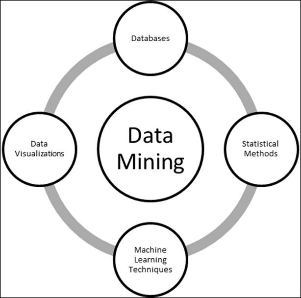
Figure 1: Data Mining - a multi-disciplinary subject

The process of data mining involves various steps:

1. Extract the required data from databases and data warehouses.

2. Perform a sanity check on the data to remove redundant characters and irrelevant information.

3. At times, it is important to combine information from various other disjoint databases. Hence, look for common attributes to combine databases.

4. Apply data transformation techniques. Sometimes, it is required to include a few attributes and features in a model.

5. Pattern recognition among the input features, where any of the pattern recognition methods can be applied.

6. Knowledge representation. This includes representation of knowledge mined from the databases in a visual form to various business stakeholders.

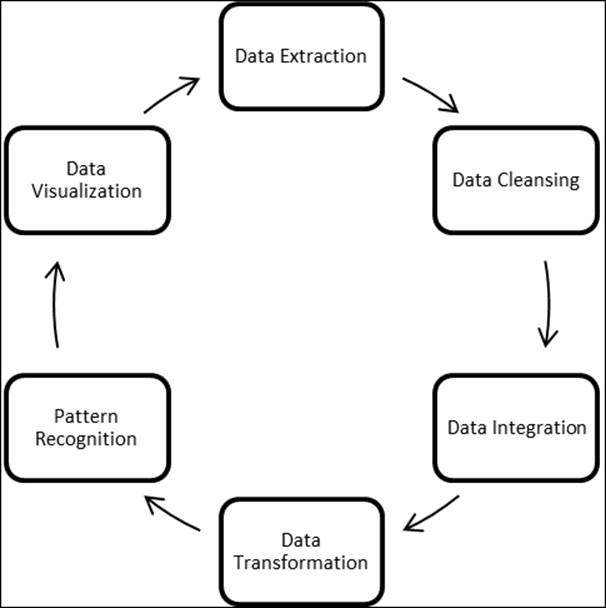
Figure 2: A typical data mining process flow

Having discussed the process flow of data mining and the core components, it is also important to look at a few challenges that one may encounter in data mining, such as computational efficiency, unstructured databases and their confluence with structured databases, high-dimensional data visualization, and so on. These issues can be resolved using innovative approaches. In this book, we are going to touch upon a few solutions while performing practical activities on our projects.

How is it related to data science, analytics, and statistical modeling?

Data science is a broader topic under which the data mining concept resides. Going by the aforementioned definition of data mining, it is a process of identifying patterns hidden in data and some interesting correlations that can provide useful insights. Data mining is a subset in data science projects that involves techniques such as pattern recognition, feature selection, clustering, supervised classification, and so on. Analytics and statistical modeling involve a wide range of predictive models-classification-based models to be applied on datasets to solve real-world business problems. There is a clear overlap between the three terminologies - data science, analytics, statistical modeling, and data mining. The three terminologies should not be looked at in isolation. Depending upon the project requirements and the kind of business problem, the overlap position might change, but at a broad level, all the concepts are well associated. The process of data mining also includes statistical and machine learning-based methods to extract data and automate rules and also represent data using good visualizations.

Introduction to the R programming language

In this chapter, we are going to start with basic programming using R for data management and data manipulation; we are also going to cover a few programming tips. R can be downloaded from https://cran.r-project.org/ . Based on the operating system, anyone can download and install R binary files on their systems. The R programming, language which is an extension of the S language, is a statistical computing platform. It provides advanced predictive modeling capability, machine learning algorithms implementation capability, and better graphical visualization. R has various other plugins such as R.Net, rJava, SparkR, and RHadoop, which increases the usability of R in big data scenarios. The user can integrate R scripts with other programming platforms. Detailed information about R can be accessed using the following link:

https://cran.r-project.org/ .

Getting started with R

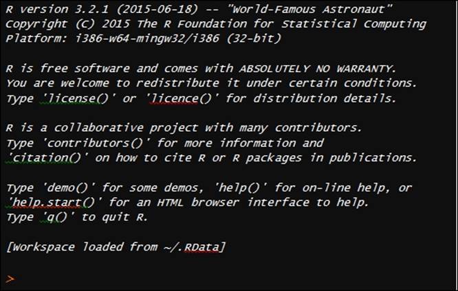
The opening message when starting R would be as shown in the preceding screenshot. Everything entered in the R console is an object, many objects created in an active R session have different attributes associated with them, and one common attribute associated with an object is called its class. There are two popular approaches to object-oriented programming in R, which are S3 classes and S4 classes. The basic difference between the S3 and S4 approaches is that the former is a more flexible approach; however, the latter is a more structured approach to object-oriented programming. Both S3 and S4 approaches recognize any symbol, character, and number as an object in R sessions and provide functionality where the object can be used for further computations.

Data types, vectors, arrays, and matrices

There are two broad sets of data types: atomic vectors and compound vectors. There are basically five data types in R programming under the atomic vector category: numeric or numbers, characters or strings, factors, logical, and complex. And there are four compound data types: data frame, lists, array, and matrix. The primary data object in R is a vector; even when we assign a single-digit number to any alphabet, it is a single element vector in R. All data objects contain a mode and a length. The mode determines the kind of data stored in the object, and the length determines the number of elements contained in that object. The c() function in R implies concatenating of various elements in a vector.

Let's take a look at various examples showing different data types in R:

> x1<-c(2.5,1.4,6.3,4.6,9.0)

> class(x1)

[1] "numeric"

> mode(x1)

[1] "numeric"

> length(x1)

[1] 5

In the preceding script, the x1 vector is a numeric vector and the number of elements is 5. Both class() and mode() return the same results, hence both determine the type of vector:

> x2<-c(TRUE,FALSE,TRUE,FALSE,FALSE)

> class(x2)

[1] "logical"

> mode(x2)

[1] "logical"

> length(x2)

[1] 5

The x2 vector is a logical vector having five elements. The logical vector elements or values can be written as either T/F or TRUE/FALSE.

> x3<-c("DataMining","Statistics","Analytics","Projects","MachineLearning")

> class(x3)

[1] "character"

> length(x3)

[1] 5

Object x3 represents a character vector of length 25. All elements of the vector can be mentioned within double quote (" ") or single quote (' ').

The factor is another form of data where various categories listed in the vector are known as levels, in the preceding example; vector a is a character vector with two levels or categories, which are repeated with some frequency. The as.factor() command is used to convert a character vector into a factor data type. After applying that, it indicates there are five levels such as Analytics, DataMining, MachineLearning, Projects, and Statistics. The table() command indicates the frequency table computed from the factor variable:

> x<-data.frame(x1,x2,x3)

> class(x)

[1] "data.frame"

> print(x)

x1 x2 x3

1 12 TRUE Analytics

2 13 FALSE DataMining

3 24 TRUE MachineLearning

4 54 FALSE Projects

5 29 TRUE Statistics

Dataframes are another popular form of data type in the R programming language that include all different data types. A dataframe is a list that contains multiple vectors of the same length and different types of data. If you simply import a dataset from a spreadsheet, the data type by default becomes dataframe. Later on, the data type for individual variables can be changed. So, dataframe can be defined as a matrix that contains columns of different data types. In the preceding script, the dataframe xcontains three different data types: numeric, logical, and character. Most real-world datasets contain different data types; for example, in a retail store, information about customers is stored in a database. This includes customer ID, purchase date, amount purchased, whether part of any loyalty program or not, and so on.

One important point about vectors: all elements of a vector should be of the same type. If not, R will forcibly convert that by coercion. For example, in a numeric vector, if one element contains a character value, the vector type will change from numeric to character. The script is given as follows:

> x1<-c(2.5,1.4,6.3,4.6,9.0)

> class(x1)

[1] "numeric"

> x1<-c(2.5,1.4,6.3,4.6,9.0,"cat")

> class(x1)

[1] "character"

R is case sensitive, so "cat" is different from "Cat". Hence, please be careful while assigning object names to the vectors. At times, it would be difficult to remember the object names:

> ls()

[1] "a" "centers" "df" "distances"

[5] "dt2" "i" "indexes" "km"

[9] "kmd" "kmeans.results" "log_model" "mtcars"

[13] "outliers" "pred" "predict.kmeans" "probs"

[17] "Smarket" "start" "sumsq" "t"

[21] "test" "Titanic" "train" "x"

[25] "x1" "x2" "x3" "x4"

[29] "x5" "y" "z"

To know what all objects are active in the current R session, the ls() command can be used; the list command will print all the active objects in the current session. Let's take a look at what a list is, how to retrieve the elements of a list, and how the list function can be used.

List management, factors, and sequences

A list is an ordered collection of objects that can contain arbitrary objects. Elements of a list can be accessed using the double square bracket. Those collections of objects are not necessarily of the same type. They can be of different types:

> mylist<-list(custid=112233, custname="John R", mobile="989-101-1011",

+ email="JohnR@gmail.com")

> mylist

$custid

[1] 112233

$custname

[1] "John R"

$mobile

[1] "989-101-1011"

$email

[1] "JohnR@gmail.com"

In the preceding example, the customer ID and mobile number are of numeric data type; however, the customer name and e-mail ID are of character data type. There are basically four elements in the preceding list. To extract elements from a list, we use double square brackets, and if we need to extract only a sublist from the list, we can use a single square bracket:

> mylist[[2]]

[1] "John R"

> mylist[2]

$custname

[1] "John R"

The next thing related to lists is how to combine more than one list. Lists can be combined using the cbind() function, that is, the column bind function:

> mylist1<-list(custid=112233, custname="John R", mobile="989-101-1011",

+ email="JohnR@gmail.com")

> mylist2<-list(custid=443322, custname="Frank S", mobile="781-101-6211",

+ email="SFranks@hotmail.com")

> mylist<-cbind(mylist1,mylist2)

> mylist

mylist1 mylist2

custid 112233 443322

custname "John R" "Frank S"

mobile "989-101-1011" "781-101-6211"

email "JohnR@gmail.com" "SFranks@hotmail.com"

Factors can be defined as various levels occurring in a categorical or nominal variable with a certain frequency. In other words, levels that are repetitive in a categorical variable are known as factors. In the following sample script, a character vector "domains" contains many levels; using the factor command, the frequency for each level can be estimated.

Sequences are repeated number of iterations, either numerical values or categorical or nominal values that can be part of a dataset. Numeric sequences can be created using a colon operator. To generate sequences using factor variables, the gl() function can be used. This is a very useful function while computing quantiles and graphical functions. Also, there are various other possible scenarios where you can use the function:

> seq(from=1,to=5,length=4)

[1] 1.000000 2.333333 3.666667 5.000000

> seq(length=10,from=-2,by=.2)

[1] -2.0 -1.8 -1.6 -1.4 -1.2 -1.0 -0.8 -0.6 -0.4 -0.2

> rep(15,10)

[1] 15 15 15 15 15 15 15 15 15 15

> gl(2,5,labels=c('Buy','DontBuy'))

[1] Buy Buy Buy Buy Buy DontBuy DontBuy DontBuy DontBuy

[10] DontBuy

Levels: Buy DontBuy

The first line of code generates the sequence in ascending order, the second line creates a reverse sequence, and the last line creates a sequence for the factor data type.

Import and export of data types

If the Windows directory path is set, to import a file into the R system, it is not required to write the complete path where the file resides. If the Windows directory path is set to some other location in your system and still you want to access the file, then the complete path needs to be given to read the file:

> getwd()

[1] "C:/Users/Documents"

> setwd("C:/Users/Documents")

Any file in the documents folder can be read without mentioning the detailed path. Hence it is always suggested to change the Windows directory to the folder where the file resides.

There are different file formats; among them, CSV or text format is the best for the R programming platform. However, we can import from other file formats:

> dt<-read.csv("E:/Datasets/hs0.csv")

> names(dt)

[1] "X0" "X70" "X4" "X1" "X1.1" "general" "X57"

[8] "X52" "X41" "X47" "X57.1"

If you are using the read.csv command, there is no need to write the header True and separator as comma, but if you are using the read.table command, it is mandatory to use. Otherwise, it will read the first variable from the dataset:

> data<- read.table("E:/Datasets/hs0.csv",header=T,sep=",")

> names(data)

[1] "X0" "X70" "X4" "X1" "X1.1" "general" "X57"

[8] "X52" "X41" "X47" "X57.1"

While mentioning paths to extract the files, you can use either / or \\; both ways will work. In real-life projects, typically data is stored in Excel format. How to read data from Excel format is a challenge. It is not always convenient to store data in CSV format and then import. The following script shows how we can import Excel files in R. Two additional libraries are required to import an RDBMS file such as Excel. Those libraries are mentioned in the script and the sample data snippets are given as well:

> library(xlsx)

Loading required package: rJava

Loading required package: xlsxjars

> library(xlsxjars)

> dat<-read.xlsx("E:/Datasets/hs0.xls","hs0")

> head(dat)

gender id race ses schtyp prgtype read write math science socst

1 0 70 4 1 1 general 57 52 41 47 57

2 1 121 4 2 1 vocati 68 59 53 63 61

3 0 86 4 3 1 general 44 33 54 58 31

4 0 141 4 3 1 vocati 63 44 47 53 56

5 0 172 4 2 1 academic 47 52 57 53 61

6 0 113 4 2 1 academic 44 52 51 63 61

Importing data from SPSS files is explained as follows. Legacy enterprise-based software systems generate data in either SPSS format or SAS format. The syntax for importing data from SPSS and SAS files needs additional packages or libraries. To import SPSS files, the Hmisc package is used, and to import SAS files, the sas7bdat library is used:

> library(Hmisc)

> mydata <- spss.get("E:/Datasets/wage.sav", use.value.labels=TRUE)

> head(mydata)

HRS RATE ERSP ERNO NEIN ASSET AGE DEP RACE SCHOOL

1 2157 2.905 1121 291 380 7250 38.5 2.340 32.1 10.5

2 2174 2.970 1128 301 398 7744 39.3 2.335 31.2 10.5

3 2062 2.350 1214 326 185 3068 40.1 2.851 NA 8.9

4 2111 2.511 1203 49 117 1632 22.4 1.159 27.5 11.5

5 2134 2.791 1013 594 730 12710 57.7 1.229 32.5 8.8

6 2185 3.040 1135 287 382 7706 38.6 2.602 31.4 10.7

> library(sas7bdat)

> mydata <- read.sas7bdat("E:/Datasets/sales.sas7bdat")

> head(mydata)

YEAR NET_SALES PROFIT

1 1990 900 123

2 1991 800 400

3 1992 700 300

4 1993 455 56

5 1994 799 299

6 1995 666 199

Exporting a dataset from R to any external location can be done by changing the read command to the write command and changing the directory path where you want to store the file.

Data type conversion

There are various types of data such as numeric, factor, character, logical, and so on. Changing one data type to another if the formatting is not done properly is not difficult at all using R. Before changing the variable type, it is essential to look at the data type it currently is. To do that, the following command can be used:

> is.numeric(x1)

[1] TRUE

> is.character(x3)

[1] TRUE

> is.vector(x1)

[1] TRUE

> is.matrix(x)

[1] FALSE

> is.data.frame(x)

[1] TRUE

When we are checking a numeric variable as numeric or not, the resultant output will display TRUE or FALSE. The same holds for other data types as well. If any data type is not right, that can be changed by the following script:

> as.numeric(x1)

[1] 2.5 1.4 6.3 4.6 9.0

> as.vector(x2)

[1] TRUE FALSE TRUE FALSE FALSE

> as.matrix(x)

x1 x2 x3 x4 x5

[1,] "2.5" " TRUE" "DataMining" "1" "1+ 0i"

[2,] "1.4" "FALSE" "Statistics" "2" "6+ 5i"

[3,] "6.3" " TRUE" "Analytics" "3" "2+ 2i"

[4,] "4.6" "FALSE" "Projects" "4" "4+ 1i"

[5,] "9.0" "FALSE" "MachineLearning" "5" "6+55i"

> as.data.frame(x)

x1 x2 x3 x4 x5

1 2.5 TRUE DataMining 1 1+ 0i

2 1.4 FALSE Statistics 2 6+ 5i

3 6.3 TRUE Analytics 3 2+ 2i

4 4.6 FALSE Projects 4 4+ 1i

5 9.0 FALSE MachineLearning 5 6+55i

> as.character(x2)

[1] "TRUE" "FALSE" "TRUE" "FALSE" "FALSE"

When using as.character(), even a logical vector is changed from logical to character vector. For a numeric variable, nothing is changed as the x1 variable was already in numeric form. A logical vector can also be changed from logical to factor using this command:

> as.factor(x2)

[1] TRUE FALSE TRUE FALSE FALSE

Levels: FALSE TRUE

Sorting and merging dataframes

Sorting and merging are two important concepts in data management. The object can be a single vector or it can be a data frame or matrix. To sort a vector in R, the sort() command is used. An decreasing order option can be used to change the order to ascending or descending. For a data frame such as ArtPiece.csv, the order command is used to sort the data, where ascending or descending order can be set for multiple variables. Descending order can be executed by putting a negative sign in front of a variable name. Let's use the dataset to explain the concept of sorting in R as shown in the following script:

> # Sorting and Merging Data

> ArtPiece<-read.csv("ArtPiece.csv")

> names(ArtPiece)

[1] "Cid" "Critic.Ratings" "Acq.Cost"

[4] "Art.Category" "Art.Piece.Size" "Border.of.art.piece"

[7] "Art.Type" "Prominent.Color" "CurrentAuctionAveragePrice"

[10] "Brush" "Brush.Size" "Brush.Finesse"

[13] "Art.Nationality" "Top.3.artists" "CollectorsAverageprice"

[16] "Min.Guarantee.Cost"

> attach(ArtPiece))

In the ArtPiece dataset, there are 16 variables: 10 numeric variables, and 6 categorical variables. Using the names command, all the names of the variables in the dataset can be printed. The attach function helps in keeping all the variable names in the current session of R, so that every time the user will not have to type the dataset name before the variable name in the code:

> sort(Critic.Ratings)

[1] 4.9921 5.0227 5.2106 5.2774 5.4586 5.5711 5.6300 5.7723 5.9789 5.9858 6.5078 6.5328

[13] 6.5393 6.5403 6.5617 6.5663 6.5805 6.5925 6.6536 6.8990 6.9367 7.1254 7.2132 7.2191

[25] 7.3291 7.3807 7.4722 7.5156 7.5419 7.6173 7.6304 7.6586 7.7694 7.8241 7.8434 7.9315

[37] 7.9576 8.0064 8.0080 8.0736 8.0949 8.1054 8.2944 8.4498 8.4872 8.6889 8.8958 8.9046

[49] 9.3593 9.8130

By default, the sorting is done by ascending order. To sort the vector based on descending order, it is required to put a negative sing before the name of the variable. The Critic.Ratings variable can also be sorted based on descending order, which is shown as follows. To sort in descending order, decreasing is true and it can be set within the command:

> sort(Critic.Ratings, decreasing = T)

[1] 9.8130 9.3593 8.9046 8.8958 8.6889 8.4872 8.4498 8.2944 8.1054 8.0949 8.0736 8.0080

[13] 8.0064 7.9576 7.9315 7.8434 7.8241 7.7694 7.6586 7.6304 7.6173 7.5419 7.5156 7.4722

[25] 7.3807 7.3291 7.2191 7.2132 7.1254 6.9367 6.8990 6.6536 6.5925 6.5805 6.5663 6.5617

[37] 6.5403 6.5393 6.5328 6.5078 5.9858 5.9789 5.7723 5.6300 5.5711 5.4586 5.2774 5.2106

[49] 5.0227 4.9921

Instead of sorting a single numeric vector, most of the times, it is required to sort a dataset based on some input variables or attributes present in the dataframe. Sorting a single variable is quite different from sorting a dataframe. The following script shows how a dataframe can be sorted using the order function:

> i2<-ArtPiece[order(Critic.Ratings,Acq.Cost),1:5]

> head(i2)

Cid Critic.Ratings Acq.Cost Art.Category Art.Piece.Size

9 9 4.9921 39200 Vintage I 26in. X 18in.

50 50 5.0227 52500 Portrait Art I 26in. X 24in.

26 26 5.2106 31500 Dark Art II 1in. X 7in.

45 45 5.2774 79345 Gothic II 9in. X 29in.

21 21 5.4586 33600 Abstract Art Type II 29in. X 29in.

38 38 5.5711 35700 Abstract Art Type III 9in. X 12in.

The preceding code shows critic ratings and acquisition cost sorted in ascending order. The order command is used instead of the sort command. The head command prints the first six observations by default from the sorted dataset. The number 1:5 in the second argument after the order command implies that we want to print the first six observations and five variables from the ArtPiece dataset. If it is required to print 10 observations from the beginning, head(i2, 10) can be executed. The dataset does not have any missing values; however, the existence of NA or missing values cannot be ruled out from any practical dataset. Hence, with the presence of NA or missing values, sorting a data frame can be tricky. So by including some arbitrary NA values in the dataset, the order command produced the following result:

> i2<-ArtPiece[order(Border.of.art.piece, na.last = F),2:6]

> head(i2)

Critic.Ratings Acq.Cost Art.Category Art.Piece.Size Border.of.art.piece

18 7.5156 34300 Vintage III 29in. X 6in.

43 6.8990 59500 Abstract Art Type II 23in. X 21in.

1 8.9046 49700 Abstract Art Type I 17in. X 27in. Border 1

12 7.5419 37100 Silhoutte III 28in. X 9in. Border 10

14 7.1254 54600 Vintage II 9in. X 12in. Border 11

16 7.2132 23100 Dark Art I 10in. X 22in. Border 11

The NA.LAST command is used to separate the missing values and NAs from the dataset. They can be either placed at the bottom of the dataset using NA.LAST is TRUE or at the beginning of the data set as NA.LAST is FALSE. By keeping NAs separate from the order function, data sanity can be maintained.

The merge function helps in combining two data frames. To combine two data frames, at least one column name should be identical. The two data frames can also be joined by using a function called column bind. To display the difference between the column bind and merge functions, we have taken audit.CSV dataset. There are two small datasets, A and B, prepared out of the audit dataset:

> A<-audit[,c(1,2,3,7,9)]

> names(A)

[1] "ID" "Age" "Employment" "Income" "Deductions"

> B<-audit[,c(1,3,4,5,6)]

> names(B)

[1] "ID" "Employment" "Education" "Marital" "Occupation"

Two columns, ID and Employment, are common in both datasets A and B, which can be used as a primary key for merging two data frames. Using the merge command, the common columns are taken once in the result dataset from the merge function. The merged data frame contains all the rows that have complete entries in both the data frames:

> head(merge(A,B),3)

ID Employment Age Income Deductions Education Marital Occupation

1 1004641 Private 38 81838.0 0 College Unmarried Service

2 1010229 Private 35 72099.0 0 Associate Absent Transport

3 1024587 Private 32 154676.7 0 HSgrad Divorced Clerical

The merge function allows four different ways of combining data: natural join, full outer join, left outer join, and right outer join. Apart from these joins, two data frames can also be merged using any specific column or multiple columns. Natural join helps to keep only rows that match from the data frames, which can be specified by the all=F argument:

> head(merge(A,B, all=F),3)

ID Employment Age Income Deductions Education Marital Occupation

1 1044221 Private 60 7568.23 0 College Married Executive

2 1047095 Private 74 33144.40 0 HSgrad Married Service

3 1047698 Private 43 43391.17 0 Bachelor Married Executive

Full outer join allows us to keep all rows from both data frames, and this can be specified by the all=T command. This performs the complete merge and fills the columns with NA values where there is no matching data in both the data frames. The default setting of the merge function drops all unmatched cases from both the data frames; to keep all the cases in new data frame, we need to specify all=T:

> head(merge(A,B, all=T),3)

ID Employment Age Income Deductions Education Marital Occupation

1 1004641 Private 38 81838.0 0 <NA> <NA> <NA>

2 1010229 Private 35 72099.0 0 <NA> <NA> <NA>

3 1024587 Private 32 154676.7 0 <NA> <NA> <NA>

Left outer join allows us to include all the rows of data frame one (A) and only those from data frame two (B) that match; to perform this, we need to specify all.x=T:

> head(merge(A,B, all.x = T),3)

ID Employment Age Income Deductions Education Marital Occupation

1 1004641 Private 38 81838.0 0 <NA> <NA> <NA>

2 1010229 Private 35 72099.0 0 <NA> <NA> <NA>

3 1024587 Private 32 154676.7 0 <NA> <NA> <NA>

Right outer join allows us to include all the rows of data frame B and only those from A that match; specify all.y=T:

> head(merge(A,B, all.y = T),3)

ID Employment Age Income Deductions Education Marital Occupation

1 1044221 Private 60 7568.23 0 College Married Executive

2 1047095 Private 74 33144.40 0 HSgrad Married Service

3 1047698 Private 43 43391.17 0 Bachelor Married Executive

In data frames A and B, two columns are common; they are ID and Employment. Using the merge command, if we select by one common variable, the other common variable would appear on the result data frame. If we select multiple data frames as the criteria to merge, then all duplicate columns from the resulting data frame will disappear:

> head(merge(A,B,by="ID"),3)

ID Age Employment.x Income Deductions Employment.y Education Marital Occupation

1 1044221 60 Private 7568.23 0 Private College Married Executive

2 1047095 74 Private 33144.40 0 Private HSgrad Married Service

3 1047698 43 Private 43391.17 0 Private Bachelor Married Executive

> head(merge(A,B,by=c("ID","Employment")),3)

ID Employment Age Income Deductions Education Marital Occupation

1 1044221 Private 60 7568.23 0 College Married Executive

2 1047095 Private 74 33144.40 0 HSgrad Married Service

3 1047698 Private 43 43391.17 0 Bachelor Married Executive

The merge function works when two data frames contain at least one common column, if both the data frames contain disjoint columns or there is no common column between the two data frames, then to combine both data frames, the column bind function can be used. The column bind function prints all the columns in data frame A and data frame B and puts them side by side:

> A<-audit[,c(2,7,9)]

> names(A)

[1] "Age" "Income" "Deductions"

> B<-audit[,c(4,5,6)]

> names(B)

[1] "Education" "Marital" "Occupation"

> head(cbind(A,B),3)

Age Income Deductions Education Marital Occupation

1 38 81838.0 0 College Unmarried Service

2 35 72099.0 0 Associate Absent Transport

3 32 154676.7 0 HSgrad Divorced Clerical

Indexing or subsetting dataframes

While working on a client dataset with a large number of observations, it is required to subset the data based on some selection criteria and with or without replacement-based sampling. Indexing is the process of extracting the subset of data from the dataframe based on some logical conditions. The subset function helps in extracting elements from the data frame like indexing:

> newdata <- audit[ which(audit$Gender=="Female" & audit$Age > 65), ]

> rownames(newdata)

[1] "49" "537" "552" "561" "586" "590" "899" "1200" "1598" "1719"

The preceding code explains: select those observations from the audit dataset where the gender is female and the age is more than 65 years. Which command is used to select that subset of data audit based on the preceding two criteria? There are 10 observations satisfying the preceding condition; the row numbers of the data frame are printed previously. A similar result can be obtained by using the subset function as well. Instead of the which function, the subset function should be used, as the latter is more efficient in passing multiple conditions. Let's take a look at the way the subset function is used:

> newdata <- subset(audit, Gender=="Female" & Age > 65, select=Employment:Income)

> rownames(newdata)

[1] "49" "537" "552" "561" "586" "590" "899" "1200" "1598" "1719"

The additional argument in the subset function makes the function more efficient as it provides the additional benefit of selecting specific columns from the dataframe where the logical condition is satisfied.

Date and time formatting

The date functions return a Date class that represents the number of days since January 1, 1970. The as.numeric() function can be used to create a numeric variable with the number of days since 1/1/1970. The return value of as.Date() is a Date class object:

> Sys.time()

[1] "2015-11-10 00:43:22 IST"

> dt<-as.Date(Sys.time())

> class(dt)

[1] "Date"

The system time function captures the date and time with the time zone. When we convert the system time using the as.Date function and stored as a new object in R, we find that the class of that object is Date. The weekdays function returns the name of the day such as "Monday" or "Wednesday". The months function returns the name of the month from the date variable. The quarters function returns the name of the quarter for the date object and year value also can be extracted using the substr() command:

> weekdays(as.Date(Sys.time()))

[1] "Monday"

> months(as.Date(Sys.time()))

[1] "November"

> quarters(as.Date(Sys.time()))

[1] "Q4"

> substr(as.POSIXct(as.Date(Sys.time())),1,4)

[1] "2015"

If the date variable given in the dataset is not in proper format for further computations, it can be formatted using the format function:

> format(Sys.time(),format = "%m %d %y")

[1] "11 10 15"

There are various options that can be passed to the format argument based on the user requirement:

Table 1: Formatting date options

Practical datasets contain date fields such as the transaction date in retail, visit date in healthcare, and processing date in BFSI; and any time series data contains at least one time element. To include the date variable in any statistical model, data transformation is required, such as calculating the vintage of a customer in a retail scenario. The data transformation can be done using the aforementioned options.

Creating new functions

There are two different types of functions in R, user-defined functions and built-in functions.

User-defined functions

A user-defined function provides customization and flexibility to users to write their functions to perform computations. It has a general notation shown as follows:

newFunc <- function(x){define function}

> int<-seq(1:20)

> int

[1] 1 2 3 4 5 6 7 8 9 10 11 12 13 14 15 16 17 18 19 20

> myfunc<-function(x){x*x}

> myfunc(int)

[1] 1 4 9 16 25 36 49 64 81 100 121 144 169 196 225 256 289 324

361 400

In the preceding script, we are creating a small sequence of numbers from 1 to 20 and a user-defined function to calculate the square of each integer. Using the new function, we can calculate the square of any number. So the user can define and create his or her own custom function.

Built-in functions

Built-in functions, such as mean, median, standard deviation, and so on, provide the user the ability to compute basic statistics using R. There are many built-in functions; the following table displays a few important built-in functions:

Table 2: Some built-in functions

Loop concepts - the for loop

The for loop is the most popular looping construct in R. Using a for loop, a similar task can be performed many times iteratively, let's look at a sample example where the for loop concept is applied. In the following code, a series of numbers from 10 to 25 is created. The null vector v is acting like a storage unit. If the condition mentioned in the following code is not met, the loop is never executed:

x<-100:200

y <- NULL # NULL vector as placeholder

for(i in seq(along=x)) {

if(x[i] < 150) {

y <- c(y, x[i] - 50)

} else {

y <- c(y, x[i] + 50)

}

}

print(y)

Loop concepts - the repeat loop

The repeat loop is used to iterate a certain calculation over a vector or dataframe. There is no provision to check the condition to exit the loop; generally a break statement is used to exit the loop. If you fail to provide any break condition within the repeat loop, you will end up running the repeat loop infinitely. Let's look at the code showing how to write a repeat loop. The break condition used in the following code is if x > 2.6:

x <- 100

repeat {

print(x)

x = sqrt(x)+10

if (x > 2.6){

break

}

}

Loop concepts - while conditions

The structure of the while loop in R is simple; it starts with a desired result that the user wants to see from the experiment. As the condition is entered in the beginning, the body of the loop will start iteration and go on as long the condition is being met. The skeleton structure of a while loop consists of a constraint condition to start with; here is an example:

x <- 10

while (x < 60) {

print(x)

x = x+10

}

If we compare different types of loops in the R programming language, for loop and while loop are very frequently used; repeat loop is not used that frequently because of the time it takes to complete the run. If we compare the loops with the apply group of functions, the latter set of functions is quite effective in handling different tasks in R. Let's look at the apply group of functions.

Apply concepts

The apply function uses an array, a matrix, or a dataframe as an input and returns the result in an array format. The calculation or operation is defined by the user's custom function or using any built-in functions. The margin argument is used to specify which margin we want to apply to the function and which margin we wish to keep. If the array we are using is a matrix, then we can specify the margin to be either 1 (apply the function to the rows) or 2 (apply the function to the columns). The function can be any function such as mean, median, standard deviation, variance, and so on that is built in or user defined. Here we are going to use iris dataset to perform the task:

> apply(ArtPiece[,2:3],2,mean)

Critic.Ratings Acq.Cost

7.200416 44440.900000

> apply(ArtPiece[,2:3],1,mean)

[1] 24854.45 26604.68 17153.69 14353.28 14003.47 19604.05 14703.27 15753.29 19602.50

[10] 26954.24 19254.00 18553.77 18903.97 27303.56 24153.74 11553.61 23804.04 17153.76

[19] 19953.30 24854.22 16802.73 20303.33 14354.91 26952.99 24503.28 15752.61 28004.45

[28] 30803.81 29403.27 19604.00 29053.88 17152.81 33253.91 24502.89 37453.92 12604.15

[37] 21353.82 17852.79 28703.83 29753.25 23453.27 18204.34 29753.45 27654.05 39675.14

[46] 24853.61 16102.99 13653.98 14353.66 26252.51

The lapply function is useful when dealing with (applying any function) dataframes. In R, the dataframe is considered a list and the variables in the dataframe are the elements of the list. We can, therefore, apply a function to all the variables in a dataframe using the lapply function:

> lapply(ArtPiece[,2:3],mean)

$Critic.Ratings

[1] 7.200416

$Acq.Cost

[1] 44440.9

The sapply function applies to elements in a list and returns the results in a vector, matrix, or list. When the argument is simplify=F, then the sapply function returns the results in a list just like the lapply function. However, when the argument is simplify=T, which is the default argument, the sapply function returns the results in a simplified form if at all possible:

> sapply(ArtPiece[,2:3],mean)

Critic.Ratings Acq.Cost

7.200416 44440.900000

When we want to apply a function to subsets of a vector and the subsets are defined by some other vector, usually a factor. The output from tapply is a matrix/array, where an element in the matrix/array is the value of f at a grouping g of the vector, and g gets pushed to the row/col names:

> head(tapply(Critic.Ratings,Acq.Cost,summary),3)

$`23100`

Min. 1st Qu. Median Mean 3rd Qu. Max.

7.213 7.213 7.213 7.213 7.213 7.213

$`25200`

Min. 1st Qu. Median Mean 3rd Qu. Max.

8.294 8.294 8.294 8.294 8.294 8.294

$`27300`

Min. 1st Qu. Median Mean 3rd Qu. Max.

7.958 7.958 7.958 7.958 7.958 7.958

There are other functions in the apply family of functions, such as:

· eapply: Apply a function over values in an environment

· mapply: Apply a function to multiple list or vector arguments

· rapply: Recursively apply a function to a list

String manipulation

String manipulation or character manipulation is an important aspect of any data management system. In a typical real-world dataset, names of customers for example are written in different ways, such as J H Smith, John h Smith, John h smith, and so on. Upon verifying, it is observed that all three names belong to the same person. In typical data management, it is important to standardize the text columns or variables in a dataset because R is case sensitive and it reads any discrepancy as a new data point. There can be many other variables such as the name/model of a vehicle, product description, and so on. Let's look how the text can be standardized using some functions:

> x<-"data Mining is not a difficult subject, anyone can master the subject"

> class(x)

[1] "character"

> substr(x, 1, 12)

[1] "data Mining "

The object X in the preceding script is a string or character object. The substr command is used to pull a sub string from the string with the position defined in the function. If certain patterns or texts need to be altered or changed, then the sub command can be used. There are four important arguments that the user needs to pass: the string in which a pattern needs to be searched, the pattern, the modified pattern that needs to be replaced, and whether case sensitivity is acceptable or not. Let's look at a sample script:

> sub("data mining", "The Data Mining", x, ignore.case =T, fixed=FALSE)

[1] "The Data Mining is not a difficult subject, anyone can master the subject"

> strsplit(x, "")

[[1]]

[1] "d" "a" "t" "a" " " "M" "i" "n" "i" "n" "g" " " "i" "s" " " "n" "o" "t" " " "a" " "

[22] "d" "i" "f" "f" "i" "c" "u" "l" "t" " " "s" "u" "b" "j" "e" "c" "t" "," " " "a" "n"

[43] "y" "o" "n" "e" " " "c" "a" "n" " " "m" "a" "s" "t" "e" "r" " " "t" "h" "e" " " "s"

[64] "u" "b" "j" "e" "c" "t"

The strsplit function helps in expanding the letters from a string. The sub command is used to alter a pattern that is not right in the string. The ignore.Case option provides the user the chance to keep the case sensitivity on or off while searching for the pattern in the defined string.

NA and missing value management

Missing value treatment is an important task in standard data mining literature. In the R programming language, missing values are represented as NA. NAs are not string or numeric values; they are considered as an indicator for missing values. After importing a dataset into the R programming platform, it is important to check whether, for any variable, missing values exist or not; to check that, the is.na() command is used. Please see the example given here:

> x<-c(12,13,14,21,23,24,NA,25,NA,0,NA)

> is.na(x)

[1] FALSE FALSE FALSE FALSE FALSE FALSE TRUE FALSE TRUE FALSE TRUE

> mean(x,na.rm=TRUE)

[1] 16.5

> mean(x)

[1] NA

Object x is a numeric vector that contains some NA values, to verify that is.na() can be used, wherever it is satisfied the result would be TRUE. If we compute anything with the presence of NA, we end up getting an error or no result. Either we can replace the data set by altering the NA values, or we can remove those NA values while performing any computation. As in the preceding script, it is na.rm=T that is used to remove the NAs from the mean computation for object x.

Missing value imputation techniques

To delete missing values from the dataset, na.omit() can be used. It removes the entire row even if the data is missing for a single variable. There are various missing value imputation methods:

· Mean imputation: The missing values in a data vector is replaced by the mean or median value of that vector, excluding the NA

· Local average method: Taking the local average for the missing value, by taking into account 3 or 5 periods moving average, that is for a 3 period the average of missing data prior value and posterior value can decide what the missing value should be

· Keeping that separate: Sometimes the imputation is simply not possible, and may be the client would be interested in keeping the missing values separate to understand the missing behavior separately

· Model-based: There are some model-based missing value imputation techniques such as the regression-based missing value prediction method

· Clustering: Similar to regression-based prediction to the missing value imputation, k-means clustering can be used to impute the missing values from the dataset

Summary

In the light of the preceding discussion, it can be summarized that data manipulation and data management is an important step in performing data mining on various live projects. Since R provides a better statistical programming platform and visualization, the use of R to explain various data mining concepts to the readers makes sense. In this chapter, we looked at an introduction to data mining and R with concepts, a few programming basics, R data types, and so on. We also covered importing and exporting of various external file formats using R, sorting and merging concepts, and missing data management techniques.

In the next chapter, we are going to learn more about performing exploratory data analysis using R and how to understand univariate, bivariate and multivariate datasets. First of all, we are going to understand the concepts, practical interpretation, and then R implementation to gain knowledge on exploratory data analysis.