R Data Mining Blueprints (2016)

Chapter 2. Exploratory Data Analysis with Automobile Data

Exploratory data analysis is an integral part of data mining. It involves numerical as well as graphical representation of variables in a dataset for easy understanding and quick conclusion about a dataset. It is important to get an understanding about the dataset, type of variables considered for analysis, association between various variables, and so on. Creating cross tabulations to understand the relationship between categorical variables and performing classical statistical tests on the data to verify various different hypotheses about the data can be tested out.

You will now get an understanding about the following things:

· How to use basic statistics to know properties of a single and multiple variables

· How to calculate correlation and association between two or more variables

· Performing multivariate data analysis

· Statistical properties of various probability functions for any dataset

· Applying statistical tests on data to conclude hypotheses

· Comparing two or more samples

Univariate data analysis

To generate univariate statistics about a dataset, we have to follow two approaches, one for continuous variables and the other for discrete or categorical variables. Univariate statistics for continuous variables includes numerical measures such as averages (mean), variance, standard deviation, quantiles, median quartiles, and so on. The mean represents each and every point in the dataset; the variance indicates the fluctuation/deviation of the individual data points from the mean, which is the center of the distribution. Quantiles are also known as percentiles, which divide the distribution into 100 equal parts. The 10^th percentile value is equivalent to 1 decile, the 25^th percentile value is equivalent to the 1^st quartile, and 75^th percentile value is equivalent to the 3^rdquartile.

There are other statistical measures of central tendency for understanding the univariate characteristics of a dataset. Median and mode are referred to as positional values, but still mode can be looked at for a continuous variable to check whether it is a bimodal series. In case of bimodal series, it is difficult to compute the center of the distribution. For ordinal data or rank data calculation of mean, representation is a good idea; it is always suggested to represent univariate statistics using median or mode. Comparison of mean, median, and mode values along with skewness, kurtosis, and standard deviation gives a clear picture about the shape of the data distribution. All of these measures of central tendency and measures of dispersion together can be calculated using a single command and also using different individual commands, which are given as follows.

Note

Here, we are going to use two datasets, diamonds.csv and Cars93.csv. Both belong to two libraries that are inbuilt in the R software for practical demo purposes.

Let's use a few commands in R to understand the data better:

> names(Cars93)

[1] "Manufacturer" "Model" "Type" "Min.Price"

[5] "Price" "Max.Price" "MPG.city" "MPG.highway"

[9] "AirBags" "DriveTrain" "Cylinders" "EngineSize"

[13] "Horsepower" "RPM" "Rev.per.mile" "Man.trans.avail"

[17] "Fuel.tank.capacity" "Passengers" "Length" "Wheelbase"

[21] "Width" "Turn.circle" "Rear.seat.room" "Luggage.room"

[25] "Weight" "Origin" "Make"

The Cars93.csv dataset contains the previously mentioned variable names and it has 27 variables and 93 observations. The variable type can be printed using the str() function:

> str(Cars93)

'data.frame': 93 obs. of 27 variables:

$ Manufacturer : Factor w/ 32 levels "Acura","Audi",..: 1 1 2 2 3 4 4 4 4 5 ...

$ Model : Factor w/ 93 levels "100","190E","240",..: 49 56 9 1 6 24 54 74 73 35 ...

$ Type : Factor w/ 6 levels "Compact","Large",..: 4 3 1 3 3 3 2 2 3 2 ...

$ Min.Price : num 12.9 29.2 25.9 30.8 23.7 14.2 19.9 22.6 26.3 33 ...

$ Price : num 15.9 33.9 29.1 37.7 30 15.7 20.8 23.7 26.3 34.7 ...

$ Max.Price : num 18.8 38.7 32.3 44.6 36.2 17.3 21.7 24.9 26.3 36.3 ...

$ MPG.city : int 25 18 20 19 22 22 19 16 19 16 ...

$ MPG.highway : int 31 25 26 26 30 31 28 25 27 25 ...

$ AirBags : Factor w/ 3 levels "Driver & Passenger",..: 3 1 2 1 2 2 2 2 2 2 ...

$ DriveTrain : Factor w/ 3 levels "4WD","Front",..: 2 2 2 2 3 2 2 3 2 2 ...

$ Cylinders : Factor w/ 6 levels "3","4","5","6",..: 2 4 4 4 2 2 4 4 4 5 ...

$ EngineSize : num 1.8 3.2 2.8 2.8 3.5 2.2 3.8 5.7 3.8 4.9 ...

$ Horsepower : int 140 200 172 172 208 110 170 180 170 200 ...

$ RPM : int 6300 5500 5500 5500 5700 5200 4800 4000 4800 4100 ...

$ Rev.per.mile : int 2890 2335 2280 2535 2545 2565 1570 1320 1690 1510 ...

$ Man.trans.avail : Factor w/ 2 levels "No","Yes": 2 2 2 2 2 1 1 1 1 1 ...

$ Fuel.tank.capacity: num 13.2 18 16.9 21.1 21.1 16.4 18 23 18.8 18 ...

$ Passengers : int 5 5 5 6 4 6 6 6 5 6 ...

$ Length : int 177 195 180 193 186 189 200 216 198 206 ...

$ Wheelbase : int 102 115 102 106 109 105 111 116 108 114 ...

$ Width : int 68 71 67 70 69 69 74 78 73 73 ...

$ Turn.circle : int 37 38 37 37 39 41 42 45 41 43 ...

$ Rear.seat.room : num 26.5 30 28 31 27 28 30.5 30.5 26.5 35 ...

$ Luggage.room : int 11 15 14 17 13 16 17 21 14 18 ...

$ Weight : int 2705 3560 3375 3405 3640 2880 3470 4105 3495 3620 ...

$ Origin : Factor w/ 2 levels "USA","non-USA": 2 2 2 2 2 1 1 1 1 1 ...

$ Make : Factor w/ 93 levels "Acura Integra",..: 1 2 4 3 5 6 7 9 8 10 ...

Calculating the univariate statistics for a few continuous (Price, MPG.city, and MPG.highway) and discrete variables (Type, AirBags, and manual transmission available) can be displayed here. You can practice the rest of the variable to get a complete understanding of the dataset.

The max() command estimates the maximum value for a variable. min() computes the minimum value. sum() calculates the total of all the values. The mean() function calculates the arithmetic average of the values, the median() function calculates the median value, and range() calculates the vector of min() and max(). var() computes the sample variance and cor() correlation between two vectors. rank() calculates the vector of the ranks of the values in a vector. The quantile() function computes a vector containing the minimum, lower quartile, median, upper quartile, and maximum of a vector.

Using the summary() function for univariate:

> summary(Cars93$Price)

Min. 1st Qu. Median Mean 3rd Qu. Max.

7.40 12.20 17.70 19.51 23.30 61.90

> summary(Cars93$MPG.city)

Min. 1st Qu. Median Mean 3rd Qu. Max.

15.00 18.00 21.00 22.37 25.00 46.00

> summary(Cars93$MPG.highway)

Min. 1st Qu. Median Mean 3rd Qu. Max.

20.00 26.00 28.00 29.09 31.00 50.00

> summary(Cars93$Type)

Compact Large Midsize Small Sporty Van

16 11 22 21 14 9

> summary(Cars93$AirBags)

Driver & Passenger Driver only None

16 43 34

> summary(Cars93$Man.trans.avail)

No Yes

32 61

Now let's look at the results of the summary function on the data frame. For a continuous variable, the numerical measures of central tendency are computed, and, for a categorical variable, the class frequencies are computed:

> summary(Cars93)

Manufacturer Model Type Min.Price

Chevrolet: 8 100 : 1 Compact:16 Min. : 6.70

Ford : 8 190E : 1 Large :11 1st Qu.:10.80

Dodge : 6 240 : 1 Midsize:22 Median :14.70

Mazda : 5 300E : 1 Small :21 Mean :17.13

Pontiac : 5 323 : 1 Sporty :14 3rd Qu.:20.30

Buick : 4 535i : 1 Van : 9 Max. :45.40

(Other) :57 (Other):87

Price Max.Price MPG.city MPG.highway

Min. : 7.40 Min. : 7.9 Min. :15.00 Min. :20.00

1st Qu.:12.20 1st Qu.:14.7 1st Qu.:18.00 1st Qu.:26.00

Median :17.70 Median :19.6 Median :21.00 Median :28.00

Mean :19.51 Mean :21.9 Mean :22.37 Mean :29.09

3rd Qu.:23.30 3rd Qu.:25.3 3rd Qu.:25.00 3rd Qu.:31.00

Max. :61.90 Max. :80.0 Max. :46.00 Max. :50.00

AirBags DriveTrain Cylinders EngineSize

Driver & Passenger:16 4WD :10 3 : 3 Min. :1.000

Driver only :43 Front:67 4 :49 1st Qu.:1.800

None :34 Rear :16 5 : 2 Median :2.400

6 :31 Mean :2.668

8 : 7 3rd Qu.:3.300

rotary: 1 Max. :5.700

Horsepower RPM Rev.per.mile Man.trans.avail

Min. : 55.0 Min. :3800 Min. :1320 No :32

1st Qu.:103.0 1st Qu.:4800 1st Qu.:1985 Yes:61

Median :140.0 Median :5200 Median :2340

Mean :143.8 Mean :5281 Mean :2332

3rd Qu.:170.0 3rd Qu.:5750 3rd Qu.:2565

Max. :300.0 Max. :6500 Max. :3755

Fuel.tank.capacity Passengers Length Wheelbase

Min. : 9.20 Min. :2.000 Min. :141.0 Min. : 90.0

1st Qu.:14.50 1st Qu.:4.000 1st Qu.:174.0 1st Qu.: 98.0

Median :16.40 Median :5.000 Median :183.0 Median :103.0

Mean :16.66 Mean :5.086 Mean :183.2 Mean :103.9

3rd Qu.:18.80 3rd Qu.:6.000 3rd Qu.:192.0 3rd Qu.:110.0

Max. :27.00 Max. :8.000 Max. :219.0 Max. :119.0

Width Turn.circle Rear.seat.room Luggage.room

Min. :60.00 Min. :32.00 Min. :19.00 Min. : 6.00

1st Qu.:67.00 1st Qu.:37.00 1st Qu.:26.00 1st Qu.:12.00

Median :69.00 Median :39.00 Median :27.50 Median :14.00

Mean :69.38 Mean :38.96 Mean :27.83 Mean :13.89

3rd Qu.:72.00 3rd Qu.:41.00 3rd Qu.:30.00 3rd Qu.:15.00

Max. :78.00 Max. :45.00 Max. :36.00 Max. :22.00

NA's :2 NA's :11

Weight Origin Make

Min. :1695 USA :48 Acura Integra: 1

1st Qu.:2620 non-USA:45 Acura Legend : 1

Median :3040 Audi 100 : 1

Mean :3073 Audi 90 : 1

3rd Qu.:3525 BMW 535i : 1

Max. :4105 Buick Century: 1

(Other) :87

The summary command for continuous variables such as RPM, horsepower, and so on shows the minimum, 1^st quartile, mean, median, 3^rd quartile, and maximum values. The univariate statistics for the categorical variable, which are car type, airbags, manual transmission availability, and so on, are represented as frequency tables. The class that has the highest frequency is considered to be the modal class.

Similar summary statistics can be generated using a few more functions such as fivenum() and describe(), which provides more information than the summary function:

> fivenum(Cars93$Price)

[1] 7.4 12.2 17.7 23.3 61.9

> fivenum(Cars93$MPG.city)

[1] 15 18 21 25 46

> fivenum(Cars93$MPG.highway)

[1] 20 26 28 31 50

The describe() function from the library (Hmisc) can be used to get a better understanding of the data description:

> library(Hmisc)

> describe(Cars93)

Cars93

27 Variables 93 Observations

Price

n missing unique Info Mean .05 .10 .25 .50 .75 .90

93 0 81 1 19.51 8.52 9.84 12.20 17.70 23.30 33.62

.95

36.74

lowest : 7.4 8.0 8.3 8.4 8.6, highest: 37.7 38.0 40.1 47.9 61.9

MPG.city

n missing unique Info Mean .05 .10 .25 .50 .75 .90

93 0 21 0.99 22.37 16.6 17.0 18.0 21.0 25.0 29.0

.95

31.4

lowest : 15 16 17 18 19, highest: 32 33 39 42 46

-----------------------------------------------------------------------------------------

MPG.highway

n missing unique Info Mean .05 .10 .25 .50 .75 .90

93 0 22 0.99 29.09 22.0 23.2 26.0 28.0 31.0 36.0

.95

37.4

lowest : 20 21 22 23 24, highest: 38 41 43 46 50

-----------------------------------------------------------------------------------------

AirBags

n missing unique

93 0 3

Driver & Passenger (16, 17%), Driver only (43, 46%)

None (34, 37%)

-----------------------------------------------------------------------------------------

Man.trans.avail

n missing unique

93 0 2

No (32, 34%), Yes (61, 66%)

The univariate summary statistics can also be calculated using the apply() function. The univariate statistics gives an impression about the shape of the distribution:

> n_cars93<-Cars93[,c(5,7,8)]

> c_cars93<-Cars93[,c(3,9,16)]

> apply(n_cars93,2,mean)

Price MPG.city MPG.highway

19.50968 22.36559 29.08602

To understand the shape of a distribution for a variable, we can use skewness and box plot. We can also use the skewness function, which is available in library(e1071):

> library(e1071)

> apply(n_cars93,2,skewness)

Price MPG.city MPG.highway

1.483982 1.649843 1.190507

We can create a custom function for measuring skewness and use that along with the apply() function:

> skewness<-function(x){

+ m3<-sum((x-mean(x))^3)/length(x)

+ s3<-sqrt(var(x))^3

+ m3/s3 }

> apply(n_cars93,2,skewness)

Price MPG.city MPG.highway

1.483982 1.649843 1.190507

Skewness is known as a measure of symmetrical distribution where the value of skewness indicates whether a distribution is positively skewed or negatively. When the value of skewness approaches 0 or is close to zero, it indicates that the distribution is symmetric and the mean, median, and mode are exactly the same. When the value of skewness is less than 0, it indicates the value of the mean is less than the mode, and this is because of availability of extreme values on the negative side of the normal distribution. When the value of skewness is greater than 0, it indicates that the value of the mean is greater than the mode, and this is because of availability of extreme values on the right-hand side of the normal distribution. Since identification of outliers and their removal is very important, the measure of skewness helps in that direction, but that is not the only way to figure out outliers. There are other methods such as boxplot, and other custom outlier detection formulas. If we look at the previous three variables, it implies that there are indications that outlier values may exist on the positive side of the normal curve for price, MPG.city, and MPG.highway variables because the skewness value is greater than 0. To verify the existence of outliers, we can take a boxplot and print the outliers.

Bivariate analysis

The relationship or association between two variables is known as bivariate analysis. There are three possible ways of looking at the relationship:

· Numeric-to-numeric relationship

· Numeric-to-categorical relationship

· Categorical-to-categorical relationship

To know the bivariate relationship between two numeric variables, typically a scatter plot is used if the two variables happen to be continuous, and a bar plot is used if one variable is categorical and the other is continuous:

> library(ggplot2)

> library(gridExtra)

> ggplot(Cars93, aes(Cars93$Price,Cars93$MPG.city))+geom_point(aes(colour=(Cars93$Type)))+geom_smooth()

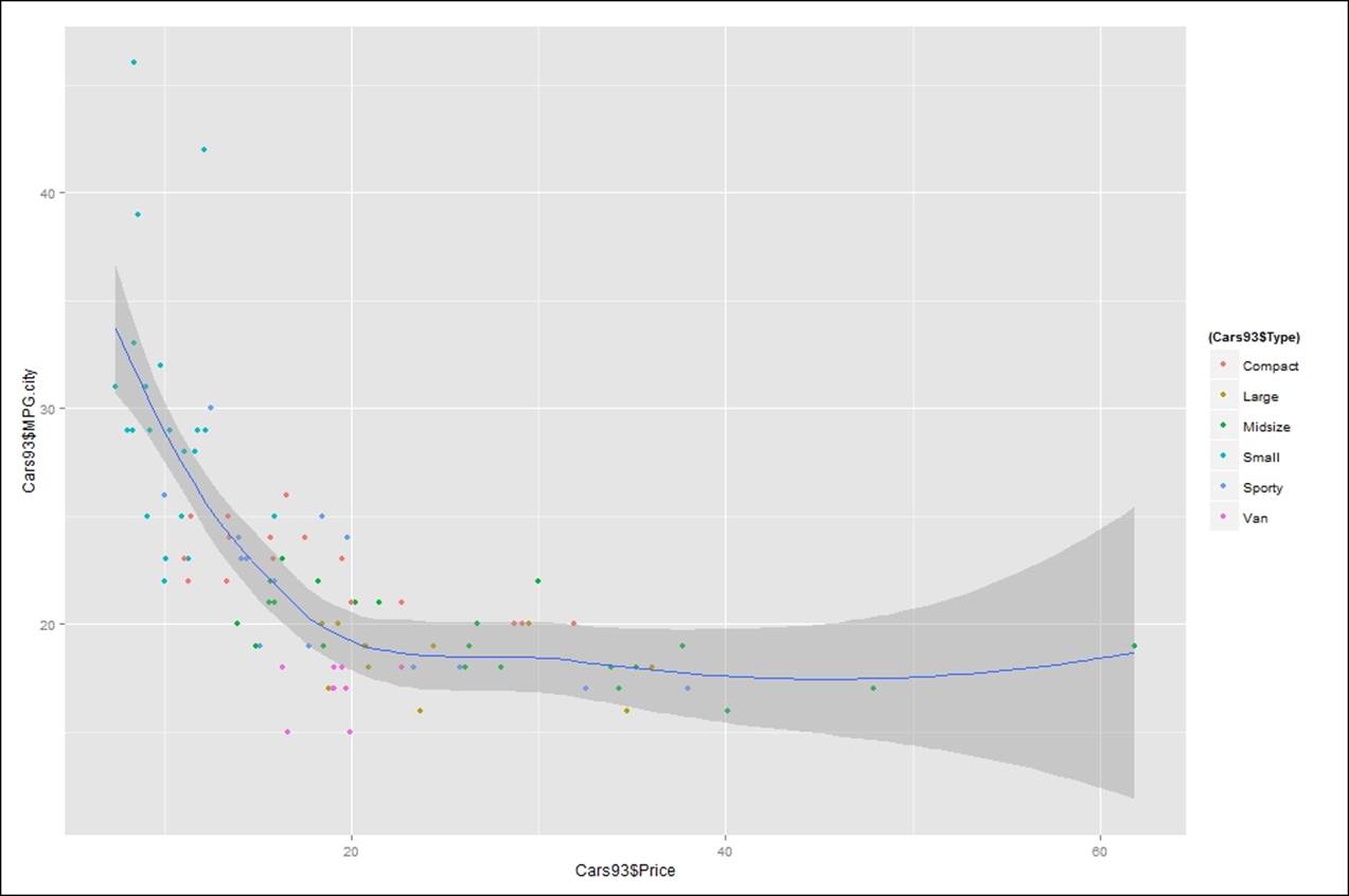
Figure 1: Showing the relationship between price and mileage within a city for different car types

Similarly, the relationship between price and highway mileage can be represented using a scatter plot as well:

> library(ggplot2)

> library(gridExtra)

> ggplot(Cars93, aes(Cars93$Price,Cars93$MPG.highway))+geom_point(aes(colour=(Cars93$Type)))+geom_smooth()

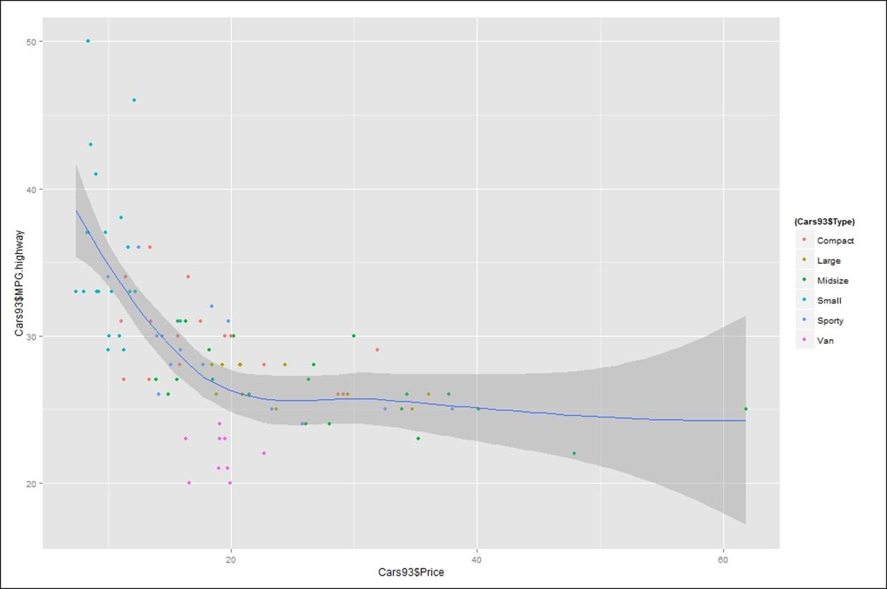
Figure 2: Relationship between price and mileage on highways

The numeric-categorical and two categorical relationships are explained in Chapter 3, Visualize Diamond Dataset, in detail.

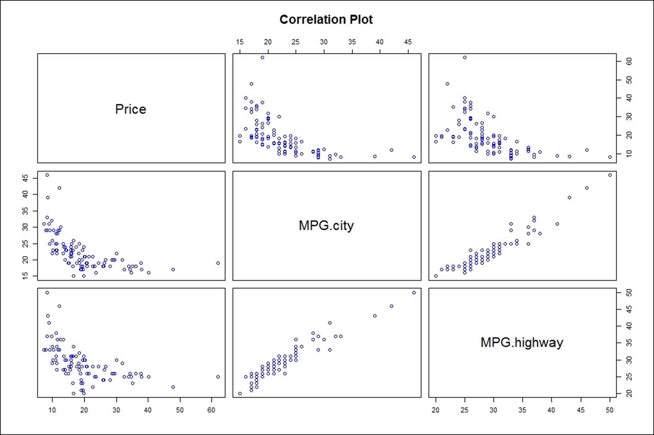
Multivariate analysis

The multivariate relationship is a statistical way of looking at multiple dependent and independent variables and their relationships. In this chapter, we will briefly talk about multivariate relationships between more than two variables, but we will discuss the details of multivariate analysis in our subsequent chapters. Multivariate relationships between various variables can be known by using the correlation method as well as cross tabulation:

> pairs(n_cars93,main="Correlation Plot", col="blue")

Understanding distributions and transformation

Understanding probability distributions is important in order to have a clear idea about the assumptions of any statistical hypothesis test. For example, in linear regression analysis, the basic assumption is that the error distribution should be normally distributed and the variables' relationship should be linear. Hence, before moving to the stage of model formation, it is important to look at the shape of the distribution and types of transformations that one may look into to make the things right. This is done so that any further statistical techniques can be applied on the variables.

Normal probability distribution

The concept of normal distribution is based on Central Limit Theorem (CLT), which implies that the population of all possible samples of size n drawn from a population with mean μ and variance σ2 approximates a normal distribution with mean μ and σ2∕nwhen n increases towards infinity. Checking the normality of variables is important to remove outliers so that the prediction process does not get influenced. Presence of outliers not only deviates the predicted values but would also destabilize the predictive model. The following sample code and example show how to check normality graphically and interpret the same.

To test out the normal distribution, we can use the mean, median, and mode for some of the variables:

> mean(Cars93$Price)

[1] 19.50968

> median(Cars93$Price)

[1] 17.7

> sd(Cars93$Price)

[1] 9.65943

> var(Cars93$Price)

[1] 93.30458

> skewness(Cars93$Price)

[1] 1.483982

ggplot(data=Cars93, aes(Cars93$Price)) + geom_density(fill="blue")

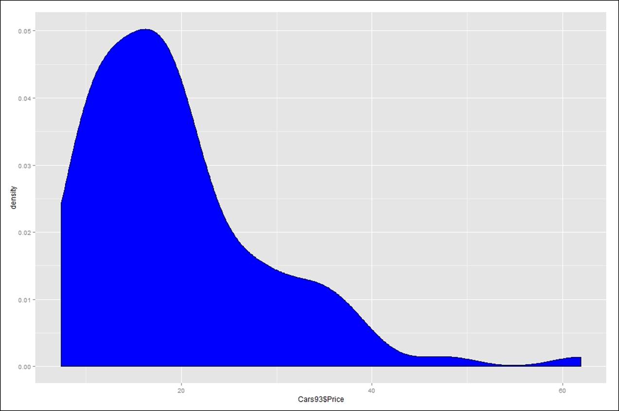
From the preceding image, we can conclude that the price variable is positively skewed because of the presence of some outlier values on the right-hand side of the distribution. The mean of the price variable is inflated and greater than the mode because the mean is subject to extreme fluctuations.

Now let's try to understand a case where normal distribution can be used to answer any hypothesis.

Suppose the variable mileage per gallon on a highway is normally distributed with a mean of 29.08 and a standard deviation of 5.33. What is the probability that a new car would provide a mileage of 35?

> pnorm(35,mean(Cars93$MPG.highway),sd(Cars93$MPG.highway),lower.tail = F)

[1] 0.1336708

Hence the required probability that a new car would provide a mileage of 35 is 13.36%, since the expected mean is higher than the actual mean; the lower tail is equivalent to false.

Binomial probability distribution

Binomial distribution is known as discrete probability distribution. It describes the outcome of an experiment. Each trial is assumed to have only two outcomes: either success or failure, either yes or no. For instance, in the Cars93 dataset variable, whether manual transmission is available or not is represented as yes or no.

Let's take an example to explain where binomial distribution can be used. The probability of a defective car given a specific component is not functioning is 0.1%. You have 93 cars manufactured. What is the probability that at least 1 defective car can be detected from the current lot of 93:

> pbinom(1,93,prob = 0.1)

[1] 0.0006293772

So the required probability that a defective car can get identified in a lot of 93 cars is 0.0006, which is very less, given the condition that the probability of a defective part is 0.10.

Poisson probability distribution

Poisson distribution is for count data where, given the data and information about an event, you can predict the probability of any number occurring within that limit using the Poisson probability distribution.

Let's take an example. Suppose 200 customers on an average visit a particular e-commerce website portal every minute. Then find the probability of having 250 customers visit the same website in a minute:

> ppois(250,200,lower.tail = F)

[1] 0.0002846214

Hence, the required probability is 0.0002, which is very rare. Apart from the aforementioned common probability distributions, which are used very frequently, there are many other distributions that can be used in rare situations.

Interpreting distributions

Calculation of probability distributions and fitting data points specific to various types of distribution and subsequent interpretation help in forming a hypothesis. That hypothesis can be used to estimate the event probability given a set of parameters. Let's take a look at the interpretation of different types of distributions.

Interpreting continuous data

The maximum likelihood estimation of the distributional parameters from any variable in a dataset can be known by fitting a distribution. The density function is available for distributions such as "beta", "cauchy", "chi-squared", "exponential", "f", "gamma", "geometric", "log-normal", "lognormal", "logistic", "negative binomial", "normal", "Poisson", "t", and "weibull". These are recognized, case being ignored. For continuous data, we will be using normal and t distributions:

> x<-fitdistr(Cars93$MPG.highway,densfun = "t")

> x$estimate

m s df

28.430527 3.937731 4.237910

> x$sd

m s df

0.5015060 0.5070997 1.9072796

> x$vcov

m s df

m 0.25150831 0.06220734 0.2607635

s 0.06220734 0.25715007 0.6460305

df 0.26076350 0.64603055 3.6377154

> x$loglik

[1] -282.4481

> x$n

[1] 93

In the preceding code, we have taken the MPG.highway variable from the Cars93 dataset. By fitting a t distribution to the variable, we obtain the parameter estimates, the estimated standard errors, the estimated variance co-variance matrix, the log likelihood value, as well as the total count. Similar activity can be performed by fitting a normal distribution to the continuous variable:

> x<-fitdistr(Cars93$MPG.highway,densfun = "normal")

> x$estimate

mean sd

29.086022 5.302983

> x$sd

mean sd

0.5498938 0.3888336

> x$vcov

mean sd

mean 0.3023831 0.0000000

sd 0.0000000 0.1511916

> x$loglik

[1] -287.1104

> x$n

[1] 93

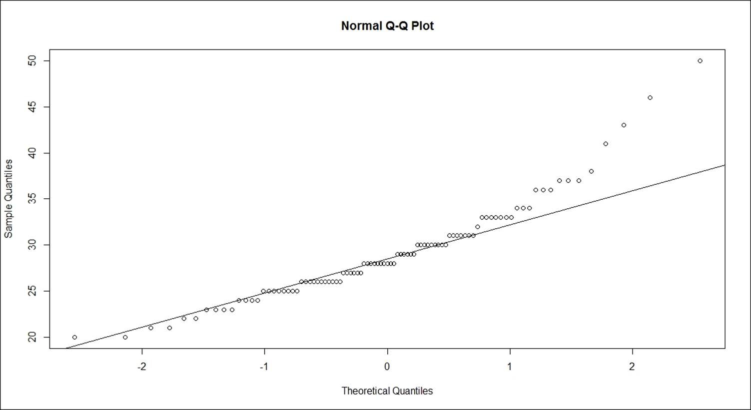
Now we are going to see how to graphically represent the variable normality:

> qqnorm(Cars93$MPG.highway)

> qqline(Cars93$MPG.highway)

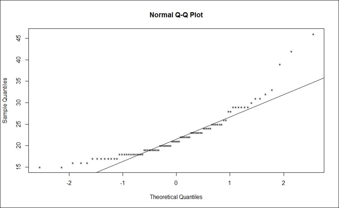
The deviation of data points represented as circles are distanced from the straight line, t.

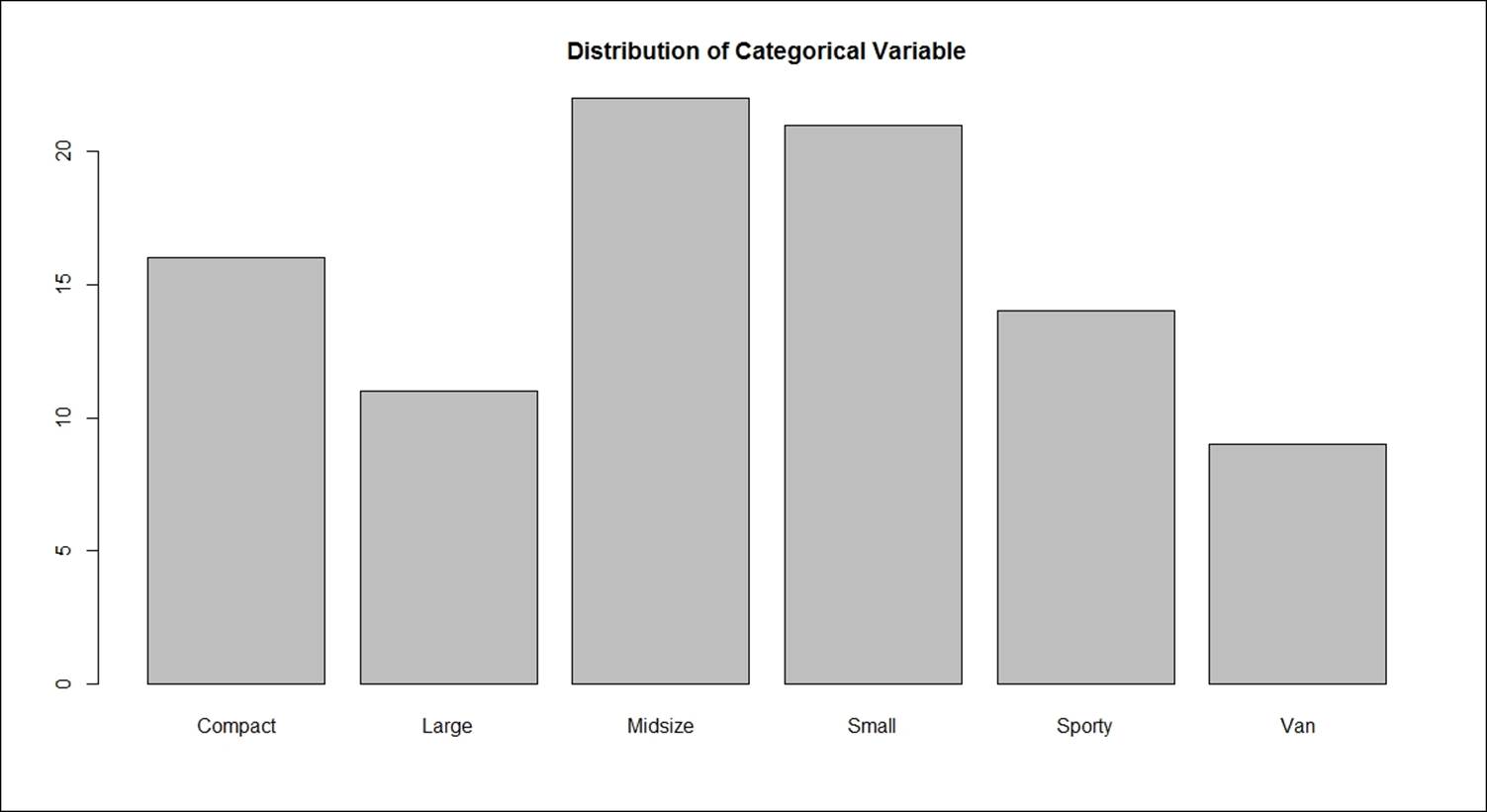
Interpreting discrete data: as all the categories in it:

> table(Cars93$Type)

Compact Large Midsize Small Sporty Van

16 11 22 21 14 9

> freq<-table(Cars93$Type)

> rel.freq<-freq/nrow(Cars93)*100

> options(digits = 2)

> rel.freq

Compact Large Midsize Small Sporty Van

17.2 11.8 23.7 22.6 15.1 9.7

> cbind(freq,rel.freq)

freq rel.freq

Compact 16 17.2

Large 11 11.8

Midsize 22 23.7

Small 21 22.6

Sporty 14 15.1

Van 9 9.7

To visualize this graphically, we need to represent it through a bar plot:

> barplot(freq, main = "Distribution of Categorical Variable")

Variable binning or discretizing continuous data

The continuous variable is the most appropriate step that one needs to take before including the variable in the model. This can be explained by taking one example fuel tank capacity of a car from the Cars93 dataset. Based on the fuel tank capacity, we can create a categorical variable with high, medium and low, lower medium:

> range(Cars93$Fuel.tank.capacity)

[1] 9.2 27.0

> cat

[1] 9.2 13.2 17.2 21.2 25.2

> options(digits = 2)

> t<-cut(Cars93$Fuel.tank.capacity,cat)

> as.data.frame(cbind(table(t)))

V1

(9.2,13.2] 19

(13.2,17.2] 33

(17.2,21.2] 36

(21.2,25.2] 3

The range of fuel tank capacity is identified as 9.2 and 27.0. Then, logically the class difference of 4 is used to arrive at classes. Those classes define how each value from the variable is assigned to each group. The final outcome table indicates that there are 4 groups; the top fuel tank capacity is available on 4 cars only.

Variable binning or discretization not only helps in decision tree construction but is also useful in the case of logistic regression mode and any other form of machine-learning-based models.

Contingency tables, bivariate statistics, and checking for data normality

Contingency tables are frequency tables represented by two or more categorical variables along with the proportion of each class represented as a group. Frequency table is used to represent one categorical variable; however, contingency table is used to represent two categorical variables.

Let's see an example to understand contingency tables, bivariate statistics, and data normality using the Cars93 dataset:

> table(Cars93$Type)

Compact Large Midsize Small Sporty Van

16 11 22 21 14 9

> table(Cars93$AirBags)

Driver & Passenger Driver only None

16 43 34

The individual frequency table for two categorical variables AirBags and Type of the car is represented previously:

> contTable<-table(Cars93$Type,Cars93$AirBags)

> contTable

Driver & Passenger Driver only None

Compact 2 9 5

Large 4 7 0

Midsize 7 11 4

Small 0 5 16

Sporty 3 8 3

Van 0 3 6

The conTable object holds the cross tabulation of two variables. The proportion of each cell in percentage is reflected in the following table. If we need to compute the row percentages or column percentages, then it is required to specify the values in the argument:

> prop.table(contTable)

Driver & Passenger Driver only None

Compact 0.022 0.097 0.054

Large 0.043 0.075 0.000

Midsize 0.075 0.118 0.043

Small 0.000 0.054 0.172

Sporty 0.032 0.086 0.032

Van 0.000 0.032 0.065

For row percentages, the value needs to be 1, and for column percentages, the value needs to be entered as 2 in the preceding command:

> prop.table(contTable,1)

Driver & Passenger Driver only None

Compact 0.12 0.56 0.31

Large 0.36 0.64 0.00

Midsize 0.32 0.50 0.18

Small 0.00 0.24 0.76

Sporty 0.21 0.57 0.21

Van 0.00 0.33 0.67

> prop.table(contTable,2)

Driver & Passenger Driver only None

Compact 0.125 0.209 0.147

Large 0.250 0.163 0.000

Midsize 0.438 0.256 0.118

Small 0.000 0.116 0.471

Sporty 0.188 0.186 0.088

Van 0.000 0.070 0.176

The summary of the contingency table performs a chi-square test of independence between the two categorical variables:

> summary(contTable)

Number of cases in table: 93

Number of factors: 2

Test for independence of all factors:

Chisq = 33, df = 10, p-value = 3e-04

Chi-squared approximation may be incorrect

The chi-square test of independence for all factors is represented previously. The message that the chi-squared approximation may be incorrect is due to the presence of null or less than 5 values in the cells of the contingency table. As in the preceding case, two random variables, car type and airbags, can be independent if the probability distribution of one variable does not impact the probability distribution of the other variable. The null hypothesis for the chi-square test of independence is that two variables are independent of each other. Since the p-value from the test is less than 0.05, at 5% level of significance we can reject the null hypothesis that the two variables are independent. Hence, the conclusion is that car type and airbags are not independent of each other; they are quite related or dependent.

Instead of two variables, what if we add one more dimension to the contingency table? Let's take Origin, and then the table would look as follows:

> contTable<-table(Cars93$Type,Cars93$AirBags,Cars93$Origin)

> contTable

, , = USA

Driver & Passenger Driver only None

Compact 1 2 4

Large 4 7 0

Midsize 2 5 3

Small 0 2 5

Sporty 2 5 1

Van 0 2 3

, , = non-USA

Driver & Passenger Driver only None

Compact 1 7 1

Large 0 0 0

Midsize 5 6 1

Small 0 3 11

Sporty 1 3 2

Van 0 1 3

The summary command for the test of independence of all factors can be used to test out the null hypothesis:

> summary(contTable)

Number of cases in table: 93

Number of factors: 3

Test for independence of all factors:

Chisq = 65, df = 27, p-value = 5e-05

Chi-squared approximation may be incorrect

Apart from the graphical methods discussed previously, there are some numerical statistical tests that can be used to know whether a variable is normally distributed or not. There is a library called norm.test for performing data normality tests, a list of functions that help in assessing the data normality from this library are listed as follows:

Let's apply the normality test on the Price variable from the Cars93 dataset:

> library(nortest)

> ad.test(Cars93$Price) # Anderson-Darling test

Anderson-Darling normality test

data: Cars93$Price

A = 3, p-value = 9e-07

> cvm.test(Cars93$Price) # Cramer-von Mises test

Cramer-von Mises normality test

data: Cars93$Price

W = 0.5, p-value = 6e-06

> lillie.test(Cars93$Price) # Lilliefors (KS) test

Lilliefors (Kolmogorov-Smirnov) normality test

data: Cars93$Price

D = 0.2, p-value = 1e-05

> pearson.test(Cars93$Price) # Pearson chi-square

Pearson chi-square normality test

data: Cars93$Price

P = 30, p-value = 3e-04

> sf.test(Cars93$Price) # Shapiro-Francia test

Shapiro-Francia normality test

data: Cars93$Price

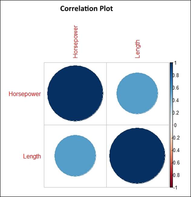
From the previously mentioned tests, it is evident that the Price variable is not normally distributed as the p-values from all the statistical tests are less than 0.05. If we add more dimensions to the bi-variate relationship, it becomes multivariate analysis. Let's try to understand the relationship between horsepower and length of a car from the Cars93 dataset:

> library(corrplot)

> o<-cor(Cars93[,c("Horsepower","Length")])

> corrplot(o,method = "circle",main="Correlation Plot")

When we include more variables, it becomes a multivariate relationship. Let's try to plot a multivariate relationship between various variables from the Cars93 dataset:

> library(corrplot)

> t<-cor(Cars93[,c("Price","MPG.city","RPM","Rev.per.mile","Width","Weight","Horsepower","Length")])

> corrplot(t,method = "ellipse")

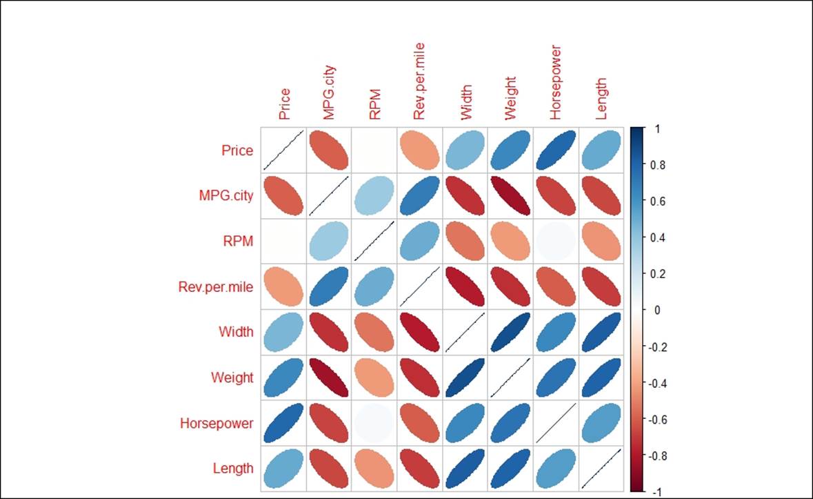
There are various methods that can be passed as an argument to the correlation plot. They are "circle", "square", "ellipse", "number", "shade", "color", and "pie".

Hypothesis testing

The null hypothesis states that nothing has happened, the means are constant, and so on. However, the alternative hypothesis states that something different has happened and the means are different about a population. There are certain steps in performing a hypothesis test:

1. State the null hypothesis: A statement about the population is assumed; for example, the average mileage of cars within a city is 40.

2. State the alternative hypothesis: If the null hypothesis turns out to be false, then what other possibility is there? For example, if the mileage within the city is not 40, then is it greater than 40 or less than 40? If it is not equal to 40, then it is a non-directional alternative hypothesis.

3. Calculate the sample test statistic: The test statistic could be t-test, f-test, z-test, and so on. Select the appropriate test statistic based on the data availability and the hypothesis declared previously.

4. Decide the confidence limit: There are three different confidence limits: 90%, 95% and 99% depending on the degree of accuracy related to a specific business problem. It is up to the researcher/analyst to choose the level of confidence interval.

5. Define the alpha value: If the confidence level selected is 95%, the alpha value is going to be 5%. Hence deciding the alpha value would help in calculating the p-value for the test.

6. Decision: If the p-value selected is less than the alpha level, then there is evidence that the null hypothesis can be rejected; if it is not, then we are going to accept the null hypothesis.

Test of the population mean

Using the hypothesis testing procedure, let's take an example from the Cars93 dataset to test out the population mean.

One tail test of mean with known variance

Suppose the researcher claims that the average mileage given by all the cars collected in the sample is more than 35. In the sample of 93 cars, it is observed that the mean mileage of all cars is 29. Should you accept or reject the researcher's claim?

The following script explains how you are going to conclude this:

Null Hypothesis: mean = 35

Alternative hypothesis= mean > 35> mu<-mean(Cars93$MPG.highway)

> mu

[1] 29

> sigma<-sd(Cars93$MPG.highway)

> sigma

[1] 5.3

> n<-length(Cars93$MPG.highway)

> n

[1] 93

> xbar= 35

> z<-(xbar-mu)/(sigma/sqrt(n))

> z

[1] 11

> #computing the critical value at 5% alpha level

> alpha = .05

> z1 = qnorm(1-alpha)

> z1

[1] 1.6

> ifelse(z > z1,"Reject the Null Hypothesis","Accept the Null Hypothesis")

Null Hypothesis: mean = 35

Alternative hypothesis= mean < 35

Two tail test of mean, with known variance:> mu<-mean(Cars93$MPG.highway)

> mu

[1] 29.09

> sigma<-sd(Cars93$MPG.highway)

> sigma

[1] 5.332

> n<-length(Cars93$MPG.highway)

> n

[1] 93

> xbar= 35

> z<-(xbar-mu)/(sigma/sqrt(n))

> z

[1] 10.7

>

> #computing the critical value at 5% alpha level

> alpha = .05

> z1 = qnorm((1-alpha)/2))

Error: unexpected ')' in "z1 = qnorm((1-alpha)/2))"

> c(-z1,z1)

[1] -1.96 1.96

>

>

> ifelse(z > z1 | z < -z1,"Reject the Null Hypothesis","Accept the Null Hypothesis")

The way we analyzed the one-tail and two-tail test of population mean for the sample data in the case of known variance.

One tail and two tail test of proportions

Using the Cars93 dataset, suppose 40% of the USA-manufactured cars have an RPM of more than 5000. From the sample data, we found that 17 out of 57 cars have RPM above 5000. What do you interpret from the context?

> mileage<-subset(Cars93,Cars93$RPM > 5000)

> table(mileage$Origin)

USA non-USA

17 40

> p1<-17/57

> p0<- 0.4

> n <- length(mileage)

> z <- (p1-p0)/sqrt(p0*(1-p0)/n)

> z

[1] -1.079

> #computing the critical value at 5% alpha level

> alpha = .05

> z1 = qnorm(1-alpha)

> z1

[1] 1.645

> ifelse(z > z1,"Reject the Null Hypothesis","Accept the Null Hypothesis")

[1] "Accept the Null Hypothesis"

If the alternative hypothesis is not directional, it is a case of two-tailed test of proportions; nothing from the preceding calculation would change except the critical value calculation. The detailed script is given as follows:

> mileage<-subset(Cars93,Cars93$RPM > 5000)

> table(mileage$Origin)

USA non-USA

17 40

> p1<-17/57

> p0<- 0.4

> n <- length(mileage)

> z <- (p1-p0)/sqrt(p0*(1-p0)/n)

> z

[1] -1.079

> #computing the critical value at 5% alpha level

> alpha = .05

> z1 = qnorm(1-alpha/2)

> c(-z1,z1)

[1] -1.96 1.96

> ifelse(z > z1 | z < -z1,"Reject the Null Hypothesis","Accept the Null Hypothesis")

[1] "Accept the Null Hypothesis"

· Two sample paired test for continuous data: The null hypothesis that is being tested in the two-sample paired test would be that there is no impact of a procedure on the subjects, the treatment has no effect on the subjects, and so on. The alternative hypothesis would be there is a statistically significant impact of a procedure, effectiveness of a treatment, or drug on the subjects.

Though we don't have such a variable in the Cars93 dataset, we can still assume the paired relationship between minimum prices and maximum prices for different brands of cars.

· Null hypothesis for the two sample t-test: There is no difference in the mean prices.

· Alternative hypothesis: There is a difference in the mean prices:

· > t.test(Cars93$Min.Price, Cars93$Max.Price, paired = T)

·

· Paired t-test

·

· data: Cars93$Min.Price and Cars93$Max.Price

·

· t = -9.6, df = 92, p-value = 2e-15

·

· alternative hypothesis: true difference in means is not equal to 0

·

· 95 percent confidence interval:

·

· -5.765 -3.781

·

· sample estimates:

·

· mean of the differences

·

· -4.773

The p-value is less than 0.05. Hence, it can be concluded that the difference in mean minimum price and maximum price is statistically significant at alpha 95% confidence level.

· Two sample unpaired test for continuous data: From the Cars93 dataset, the mileage on the highway and within the city is assumed to be different. If the difference is statistically significant, can be tested by using the independent samples t-test for comparison of means.

· Null hypothesis: There is no difference in the MPG on highway and MPG within city.

· Alternative hypothesis: There is a difference in the MPG on highway and MPG within city:

· Welch Two Sample t-test

·

· data: Cars93$MPG.city and Cars93$MPG.highway

·

· t = -8.4, df = 180, p-value = 1e-14

·

· alternative hypothesis: true difference in means is not equal to 0

·

· 95 percent confidence interval:

·

· -8.305 -5.136

·

· sample estimates:

·

· mean of x mean of y

·

· 22.37 29.09

From the two samples t-test, when the two samples are independent, the p-value is less than 0.05; hence, we can reject the null hypothesis that there is no difference in the mean mileage on highway and within city. There is a statistically significant difference in the mean mileage within city and on highway. This can be represented in a slightly different way, by putting a null hypothesis is the mean mileage difference within city is different for manual versus automatic cars:

, data=Cars93)

Welch Two Sample t-test

data: Cars93$MPG.city by Cars93$Man.trans.avail

t = -6, df = 84, p-value = 4e-08

alternative hypothesis: true difference in means is not equal to 0

95 percent confidence interval:

-6.949 -3.504

sample estimates:

mean in group No mean in group Yes

18.94 24.16

So, the conclusion from the preceding test is that there is a statistically significant difference in the mean mileage between automatic and manual transmission vehicle types; this is because the p-value is less than 0.05.

Before applying t-test, it is important to check the data normality; normality of a variable can be assessed using the Shapiro test function:

> shapiro.test(Cars93$MPG.city)

Shapiro-Wilk normality test

data: Cars93$MPG.city

W = 0.86, p-value = 6e-08

)

> qqline(Cars93$MPG.city)

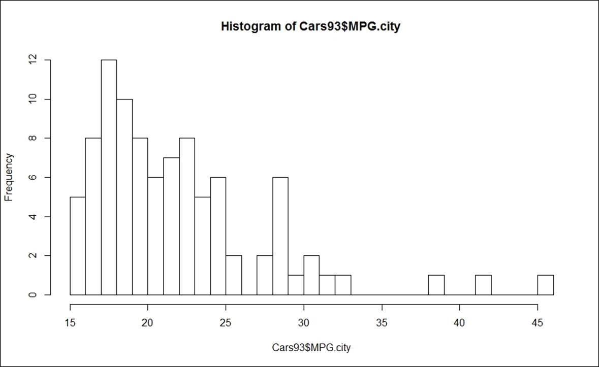
Looking at the QQ plot for the lineage per gallon within city and the histogram, it can be concluded that the variable is not normally distributed. Since the mileage variable is not normally distributed, it is required to apply non-parametric methods such as Wilcoxon signed rank test or Kolmogorov-Smirnov test.

Two sample variance test

To compare the variances of two samples, F-test is used as a statistic:

> var.test(Cars93$MPG.highway~Cars93$Man.trans.avail, data=Cars93)

F test to compare two variances

data: Cars93$MPG.highway by Cars93$Man.trans.avail

F = 0.24, num df = 31, denom df = 60, p-value = 5e-05

alternative hypothesis: true ratio of variances is not equal to 1

95 percent confidence interval:

0.1330 0.4617

sample estimates:

ratio of variances

0.2402

Since the p-value is less than 0.05, we can reject the null hypothesis that there is no difference in the variance of mileage on a highway for manual and automatic cars. This implies there is a statistically significant difference in the variance of two samples at 95% confidence level.

The variances of the two groups can also be tested using Bartlett test:

> bartlett.test(Cars93$MPG.highway~Cars93$Man.trans.avail, data=Cars93)

Bartlett test of homogeneity of variances

data: Cars93$MPG.highway by Cars93$Man.trans.avail

Bartlett's K-squared = 17, df = 1, p-value = 4e-05

From the preceding test, it can also be concluded that the null hypothesis of equal variances can be rejected at alpha 0.05 level, and it can be proven that there is a statistically significant difference in the variance of the two samples.

One-way ANOVA:, one-way ANOVA can be used. The variable considered is RPM, and the grouping variable considered is Cylinders.

Null hypothesis: There is no difference in the means of RPM across different cylinder types.

Alternative hypothesis: There is a difference in the mean RPM for at least one cylinder type:

> aov(Cars93$RPM~Cars93$Cylinders)

Call:

aov(formula = Cars93$RPM ~ Cars93$Cylinders)

Terms:

Cars93$Cylinders Residuals

Sum of Squares 6763791 25996370

Deg. of Freedom 5 87

Residual standard error: 546.6

Estimated effects may be unbalanced

> summary(aov(Cars93$RPM~Cars93$Cylinders))

Df Sum Sq Mean Sq F value Pr(>F)

Cars93$Cylinders 5 6763791 1352758 4.53 0.001 **

Residuals 87 25996370 298809

---

Signif. codes: 0 '***' 0.001 '**' 0.01 '*' 0.05 '.' 0.1 ' ' 1

From the preceding ANOVA, the p-value is less than 0.05; hence, the null hypothesis can be rejected. That means at least for one cylinder type, the mean RPM is statistically significantly different. To identify which cylinder type is different, a post hoc test can be performed on the results of the ANOVA model:

> TukeyHSD(aov(Cars93$RPM~Cars93$Cylinders))

Tukey multiple comparisons of means

95% family-wise confidence level

Fit: aov(formula = Cars93$RPM ~ Cars93$Cylinders)

$`Cars93$Cylinders`

diff lwr upr p adj

4-3 -321.8 -1269.23 625.69 0.9201

5-3 -416.7 -1870.88 1037.54 0.9601

6-3 -744.1 -1707.28 219.11 0.2256

8-3 -895.2 -1994.52 204.04 0.1772

rotary-3 733.3 -1106.11 2572.78 0.8535

5-4 -94.9 -1244.08 1054.29 0.9999

6-4 -422.3 -787.90 -56.74 0.0140

8-4 -573.5 -1217.14 70.20 0.1091

rotary-4 1055.1 -554.08 2664.28 0.4027

6-5 -327.4 -1489.61 834.77 0.9629

8-5 -478.6 -1755.82 798.67 0.8834

rotary-5 1150.0 -801.03 3101.03 0.5240

8-6 -151.2 -817.77 515.47 0.9857

rotary-6 1477.4 -141.08 3095.92 0.0941

rotary-8 1628.6 -74.42 3331.57 0.0692

Wherever the p-adjusted value is less than 0.05, the mean difference in RPM is statistically significantly different from other groups.

Two way ANOVA with post hoc tests: The factors considered are origin and airbags. The hypothesis that needs to be tested is: is there any impact of both the categorical variables on the RPM variable?

> aov(Cars93$RPM~Cars93$Origin + Cars93$AirBags)

Call:

aov(formula = Cars93$RPM ~ Cars93$Origin + Cars93$AirBags)

Terms:

Cars93$Origin Cars93$AirBags Residuals

Sum of Squares 8343880 330799 24085482

Deg. of Freedom 1 2 89

Residual standard error: 520.2

Estimated effects may be unbalanced

> summary(aov(Cars93$RPM~Cars93$Origin + Cars93$AirBags))

Df Sum Sq Mean Sq F value Pr(>F)

Cars93$Origin 1 8343880 8343880 30.83 2.9e-07 ***

Cars93$AirBags 2 330799 165400 0.61 0.54

Residuals 89 24085482 270623

---

Signif. codes: 0 '***' 0.001 '**' 0.01 '*' 0.05 '.' 0.1 ' ' 1

> TukeyHSD(aov(Cars93$RPM~Cars93$Origin + Cars93$AirBags))

Tukey multiple comparisons of means

95% family-wise confidence level

Fit: aov(formula = Cars93$RPM ~ Cars93$Origin + Cars93$AirBags)

$`Cars93$Origin`

diff lwr upr p adj

non-USA-USA 599.4 384.9 813.9 0

$`Cars93$AirBags`

diff lwr upr p adj

Driver only-Driver & Passenger -135.74 -498.8 227.4 0.6474

None-Driver & Passenger -25.68 -401.6 350.2 0.9855

None-Driver only 110.06 -174.5 394.6 0.6280

Non-parametric methods

When a training dataset does not conform to any specific probability distribution because of non-adherence to the assumptions of that specific probability distribution, the only option left to analyze the data is via non-parametric methods. Non-parametric methods do not follow any assumption regarding the probability distribution. Using non-parametric methods, one can draw inferences and perform hypothesis testing without adhering to any assumptions. Now let's look at a set of on-parametric tests that can be used when a dataset does not conform to the assumptions of any specific probability distribution.

Wilcoxon signed-rank test

If the assumption of normality is violated, then it is required to apply non-parametric methods in order to answer a question such as: is there any difference in the mean mileage within the city between automatic and manual transmission type cars?

> wilcox.test(Cars93$MPG.city~Cars93$Man.trans.avail, correct = F)

Wilcoxon rank sum test

data: Cars93$MPG.city by Cars93$Man.trans.avail

W = 380, p-value = 1e-06

alternative hypothesis: true location shift is not equal to 0

The argument paired can be used if the two samples happen to be matching pairs and the samples do not follow the assumptions of normality:

> wilcox.test(Cars93$MPG.city, Cars93$MPG.highway, paired = T)

Wilcoxon signed rank test with continuity correction

data: Cars93$MPG.city and Cars93$MPG.highway

V = 0, p-value <2e-16

alternative hypothesis: true location shift is not equal to 0

Mann-Whitney-Wilcoxon test

If two samples are not matched, are independent, and do not follow a normal distribution, then it is required to use Mann-Whitney-Wilcoxon test to test the hypothesis that the mean difference in the two samples are statistically significantly different from each other:

> wilcox.test(Cars93$MPG.city~Cars93$Man.trans.avail, data=Cars93)

Wilcoxon rank sum test with continuity correction

data: Cars93$MPG.city by Cars93$Man.trans.avail

W = 380, p-value = 1e-06

alternative hypothesis: true location shift is not equal to 0

Kruskal-Wallis test

To compare means of more than two groups, that is, the non-parametric side of ANOVA analysis, we can use the Kruskal-Wallis test. It is also known as a distribution-free statistical test:

> kruskal.test(Cars93$MPG.city~Cars93$Cylinders, data= Cars93)

Kruskal-Wallis rank sum test

data: Cars93$MPG.city by Cars93$Cylinders

Kruskal-Wallis chi-squared = 68, df = 5, p-value = 3e-13

Summary

Exploratory data analysis is an important activity in almost all types of data mining projects. Understanding the distribution, shape of the distribution, and vital parameters of the distribution, is very important. Preliminary hypothesis testing can be done to know the data better. Not only the distribution and its properties but also the relationship between various variables is important. Hence in this chapter, we looked at bivariate and multivariate relationships between various variables and how to interpret the relationship. Classical statistical tests, such as t-test, F-test, z-test and other non-parametric tests are important to test out the hypothesis. The hypothesis testing itself is also important to draw conclusions and insights from the dataset.

In this chapter we discussed various statistical tests, their syntax, interpretations, and situations where we can apply those tests. After performing exploratory data analysis, in the next chapter we are going to look at various data visualization methods to get a 360-degree view of data. Sometimes, a visual story acts as the simplest possible representation of data. In the next chapter, we are going to use some inbuilt datasets with different libraries to create intuitive visualizations.