R Data Mining Blueprints (2016)

Chapter 5. Market Basket Analysis with Groceries Data

Think about a scenario from a retailer or e-commerce store manager when it comes to recommending the right products to customers. Product recommendation is one important domain in data mining practice. Product recommendation can happen in three different ways: by associating customer's behavior with their purchase history, by associating items that are being purchased on each visit, and lastly by looking at the gross sales in each category and then using the retailer's past experience. In this chapter, we will be looking at the second method of product recommendation, popularly known as Market Basket Analysis (MBA) also known as association rules, which is by associating items purchased at transaction level and finding out the sub-segments of users having similar products and hence, recommending the products.

In this chapter, we will cover the following topics:

· What is MBA

· Where to apply MBA

· Assumptions/prerequisites

· Modeling techniques

· Limitations

· Practical project

Introduction to Market Basket Analysis

Is MBA limited to retail and e-commerce domain only? Now, let's think about the problems where MBA or association rules can be applied to get useful insights:

· In the healthcare sector, particularly medical diagnosis, as an example, having high blood pressure and being diabetic is a common combination. So it can be concluded that people having high blood pressure are more likely to be diabetic and vice versa. Hence, by analyzing the prevalence of medical conditions or diseases, it can be said what other diseases they may likely get in future.

· In retail and e-commerce, promotions and campaigns can be designed once a merchandiser knows the relationship between the purchase patterns of different items. MBA provides insights into the relationship between various items so that product recommendation can be designed.

· In banking and financial services also, MBA can be used. Taking into account the number of products a bank is offering to the customers, such as insurance policies, mutual funds, loans, and credit cards, is there any association between buying insurance policies and mutual funds? If yes, that can be explored using market basket analysis. Before recommending a product, the officer/agent should verify what all products go together so that the upsell and cross-sell of financial products can be designed.

· In the telecommunication domain, analysis of customer usage and selection of product options provide insights into effective designing of promotions and cross-selling of products.

· In unstructured data analysis, particularly in text mining, what words go together in which domain and how the terminologies are related and used by different people can be extracted using association rules.

What is MBA?

Market Basket Analysis is the study of relationships between various products and products that are purchased together or in a series of transactions. In standard data mining literature, the task of market basket analysis is to discover actionable insights in transactional databases. In order to understand MBA or association rules (arules), it is important to understand three concepts and their importance in deciding rules:

· Support: A transaction can contain a single item or a set of items. Consider the item set x = {bread, butter, jam, curd}; the support of x implies the proportion of transactions when all four items are purchased together to the total number of transactions in the database:

Support of X = number of transactions involving X / total number of transactions

· Confidence: Confidence always refers to the confidence of a rule. It can be defined as confidence of x => y. Hence, support (x U y) implies the number of transactions in the database containing both item set x and item y:

Confidence of X => Y = support of (X U Y) / support of (X)

· Lift: Lift can be defined as the proportion of observed support to expected support:

Lift of a rule X => Y = support of (X U Y) / support of (X) * support of (Y)

An association rule stands supported in a transactional database if it satisfies the minimum support and minimum confidence criteria.

Let's take an example to understand the concepts.

The following is an example from the Groceries.csv dataset from the arules library in R:

The support of item set X where X = {milk, banana} = proportion of transactions where milk and banana bought together; 4/6 = 0.67, hence, the support of the X item set is 0.67.

Let's assume Y is curd; the confidence of X => Y, which is {milk, banana} => {curd}, is the proportion of support (X U Y) / support(X); three products--milk, banana, and curd--are purchased together 2 times. Hence the confidence of the rule = (2/6)/0.67 = 0.5. This implies that 50% of the transactions containing milk and banana the rule are correct.

Confidence of a rule can be interpreted as a conditional probability of purchasing Y such that the item set X has already been purchased.

When we create too many rules in a transactional database, we need a measure to rank the rules; lift is a measure to rank the rules. From the preceding example, we can calculate the lift for the rule X to Y. Lift of X => Y = support of (X U Y) / support of (X) * support of (Y) = 0.33/0.66*0.66 = 0.33/0.4356 = 0.7575.

Where to apply MBA?

To understand the relationship between various variables in large databases, it is required to apply market basket analysis or association rules. It is the simplest possible way to understand the association. Though we have explained various industries where the concept of association rule can be applied, the practical implementation depends on the kind of dataset available and the length of data available. For example, if you want to study the relationship between various sensors integrated at a power generation plant to understand which all sensors are activated at a specific temperature level (very high), you may not find enough data points. This is because very high temperature is a rare event and to understand the relationship between various sensors, it is important to capture large data at that temperature level.

Data requirement

Product recommendation rules are generated from the results of the association rule model. For example, what is the customer going to buy next if he/she has already added a Coke, a chips packet, and a candle? To generate rules for product recommendation, we need frequent item sets and hence the retailer can cross-sell products. Therefore the input data format should be transactional, which in real-life projects sometimes happens and sometimes does not. If the data is not in transaction form, then a transformation needs to be done. In R, dataframe is a representation of mixed data. Can we transform the dataframe to transactional data so that we can apply association rules on that transformed dataset? This is because the algorithm requires that the input data format be transactional. Let's have a look at the methods to read transactions from a dataframe.

The arules library in R provides a function to read transactions from a dataframe. This function provides two options, single and basket. In single format, each line represents a single item; however, in basket format, each line represents a transaction comprising item levels and separated by a comma, space, or tab. For example:

> ## create a basket format

> data <- paste(

+ "Bread, Butter, Jam",

+ "Bread, Butter",

+ "Bread",

+ "Butter, Banana",

+ sep="\n")

> cat(data)

Bread, Butter, Jam

Bread, Butter

Bread

Butter, Banana

> write(data, file = "basket_format")

>

> ## read data

> library(arules)

> tr <- read.transactions("basket_format", format = "basket", sep=",")

> inspect(tr)

items

1 {Bread,Butter,Jam}

2 {Bread,Butter}

3 {Bread}

4 {Banana,Butter}

Now let's look at single format transactional data creation from a dataframe:

> ## create single format

> data <- paste(

+ "trans1 Bread",

+ "trans2 Bread",

+ "trans2 Butter",

+ "trans3 Jam",

+ sep ="\n")

> cat(data)

trans1 Bread

trans2 Bread

trans2 Butter

trans3 Jam

> write(data, file = "single_format")

>

> ## read data

> tr <- read.transactions("single_format", format = "single", cols = c(1,2))

> inspect(tr)

items transactionID

1 {Bread} trans1

2 {Bread,Butter} trans2

3 {Jam} trans3

The preceding code explains how a typical piece of transactional data received in a tabular format, just like the spreadsheet format equivalent of R dataframe, can be converted to a transactional data format as required by the arules input data format.

Assumptions/prerequisites

Implementation of association rules for performing market basket analysis is based on some assumptions. Here are the assumptions:

· Assume that all data is categorical.

· There should not be any sparse data; the sparsity percentage should be minimum. Sparsity implies a lot of cells in a dataset with no values (with blank cells).

· The number of transactions required to find an interesting relationship between various products is a function of the number of items or products covered in the database. In other words, if you include more products with a less number of transactions, you will get higher sparsity in the dataset and vice versa.

· The higher the number of items you want to include in the analysis, the more number of transactions you will need to validate the rules.

Modeling techniques

There are two algorithms that are very popular for finding frequent item sets that exist in a retail transactional database:

· Apriori algorithm: It was developed by Agrawal and Srikant (1994). It considers the breadth first and provides counts of transactions.

· Eclat algorithm: This was developed by Zaki et. al. (1997b). It considers depth first; it provides intersection of transactions rather than count of transactions.

In this chapter, we are using the Groceries.csv dataset, which will be used in both the algorithms.

Limitations

Though association rules are a top choice among practitioners when it comes to understanding relationships in a large transactional database, they have certain inherent limitations:

· Association rule mining is a probabilistic approach in the sense that it computes the conditional probability of a product being purchased, such that a set of other items has already been purchased/added to the cart by the customer. It only estimates the likelihood of buying the product. The exact accuracy of the rule may or may not be true.

· Association rule is a conditional probability estimation method using simple count of items as a measure.

· Association rules are not useful practically, even with a high support, confidence, and lift; this is because most of the times, trivial rules may sound genuine. There is no mechanism to filter out the trivial rules from the global set of rules but using a machine learning framework (which is out of the scope of this book).

· The algorithm provides a large set of rules; however, a few of them are important, and there is no automatic method to identify the number of useful rules.

Practical project

The Groceries.csv dataset that we are going to use comprises of 1 month of real-world point-of-sale (POS) transaction data from a grocery store. The dataset encompasses 9,835 transactions and there are 169 categories. Item sets are defined as a combination of items or products P_i {i =1.....n} that customers buy on the same visit. To put it in a simpler way, the item sets are basically the grocery bills that we usually get while shopping from a retail store. The bill number is considered the transaction number and the items mentioned in that bill are considered the market basket. A snapshot of the dataset is given as follows:

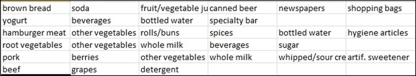
The columns represent items and the rows represent transactions in the sample snapshot just displayed. Let's explore the dataset to understand the features:

> # Load the libraries

> library(arules)

> library(arulesViz)

> # Load the data set

> data(Groceries) #directly reading from library

> Groceries<-read.transactions("groceries.csv",sep=",") #reading from local computer

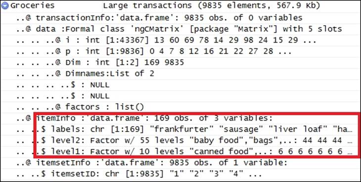
The transactional dataframe contains three columns. The first column represents the name of the product/item, the second column represents the level2 categorization of the products with 55 levels, and the third variable is the level3 segment of the product with 10 categories. This screenshot makes it clearer:

The summary of a transactional data provides an idea about the total transactions existing in the database, number of items that are part of the database, sparsity of the data, and also the frequency of the top few items prominent in the transactional database:

summary(Groceries)

transactions as itemMatrix in sparse format with

9835 rows (elements/itemsets/transactions) and

169 columns (items) and a density of 0.02609146

most frequent items:

whole milk other vegetables rolls/buns soda yogurt

2513 1903 1809 1715 1372

(Other)

34055

There are 9,835 transactions in the dataset; out of 169 items, the most frequent items with their corresponding frequencies are previously represented. In a matrix of 9,835 cross 169, only 0.0261 or 2.61% of the cells are filled with values; the rest are empty. This 2.61% is the sparsity of the dataset.

Element (itemset/transaction) length distribution:

sizes

1 2 3 4 5 6 7 8 9 10 11 12 13 14 15 16 17

2159 1643 1299 1005 855 645 545 438 350 246 182 117 78 77 55 46 29

18 19 20 21 22 23 24 26 27 28 29 32

14 14 9 11 4 6 1 1 1 1 3 1

Min. 1st Qu. Median Mean 3rd Qu. Max.

1.000 2.000 3.000 4.409 6.000 32.000

includes extended item information - examples:

labels

1 abrasive cleaner

2 artif. sweetener

3 baby cosmetics

From the preceding item set length distribution, it can be interpreted that there is one transaction with 32 products bought together. There are 3 transactions with 29 items purchased together. Likewise, we can interpret the frequency of other item sets in the dataset. This can be better understood using the item frequency plot. To know the first three transactions from the dataset, we can use the following command:

> inspect(Groceries[1:3])

items

1 {citrus fruit,semi-finished bread,margarine,ready soups}

2 {tropical fruit,yogurt,coffee}

3 {whole milk}

To know the proportion of transactions containing each item in the groceries database, we can use the following command. The first item, frankfurter, is available in 5.89% of the transactions; sausage is available in 9.39% of the transactions; and so on and so forth:

> cbind(itemFrequency(Groceries[,1:10])*100)

[,1]

frankfurter 5.8973055

sausage 9.3950178

liver loaf 0.5083884

ham 2.6029487

meat 2.5826131

finished products 0.6507372

organic sausage 0.2236909

chicken 4.2907982

turkey 0.8134215

pork 5.7651246

Two important parameters dictate the frequent item sets in a transactional dataset, support and confidence. The higher the support the lesser would be the number of rules in a dataset, and you would probably miss interesting relationships between various variables and vice versa. Sometimes with a higher support, confidence, and lift values also, it is not guaranteed to get useful rules. Hence, in practice, a user can experiment with different levels of support and confidence to arrive at meaningful rules. Even at sufficiently good amounts of minimum support and minimum confidence levels, the rules seem to be quite trivial.

To address the issue of irrelevant rules in frequent item set mining, closed item set mining is considered as a method. An item set X is said to be closed if no superset of it has the same support as X and X is maximal at % support if no superset of X has at least % support:

> itemFrequencyPlot(Groceries, support=0.01, main="Relative ItemFreq Plot",

+ type="absolute")

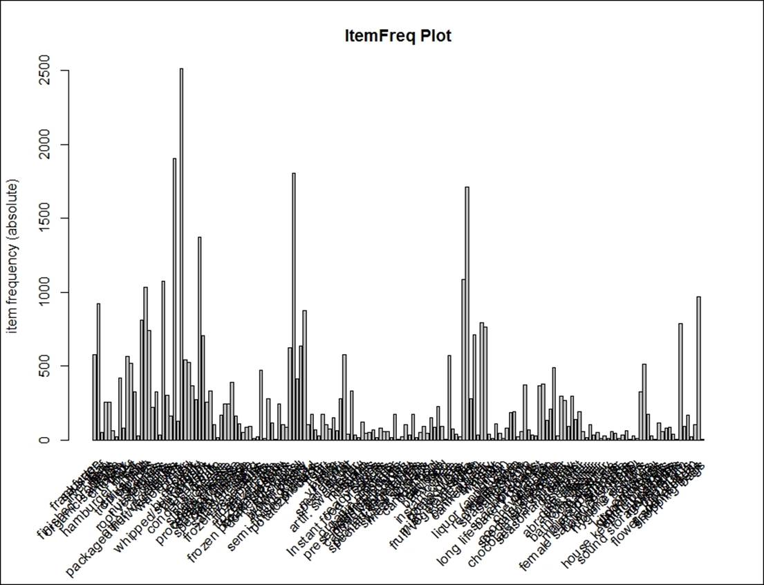
In the preceding graph, the item frequency in the absolute count is shown with a minimum support of 0.01. The following graph indicates the top 50 items with relative percentage count, showing what percentage of transactions in the database contain those items:

> itemFrequencyPlot(Groceries,topN=50,type="relative",main="Relative Freq Plot")

Apriori algorithm

Apriori algorithm uses a downward closure property, which states that any subsets of a frequent item set and also frequent item sets. The apriori algorithm uses level-wise search for frequent item sets. This algorithm only creates rules with one item in the right-hand side of the equation (RHS), which is known as consequent; left-hand side of the equation (LHS) known as antecedent. This implies that rules with one item in RHS and blank LHS may appear as valid rules; to avoid these blank rules, the minimum length parameter needs to be changed from 1 to 2:

> # Get the association rules based on apriori algo

> rules <- apriori(Groceries, parameter = list(supp = 0.01, conf = 0.10))

Parameter specification:

confidence minval smax arem aval originalSupport support minlen maxlen target ext

0.1 0.1 1 none FALSE TRUE 0.01 1 10 rules FALSE

Algorithmic control:

filter tree heap memopt load sort verbose

0.1 TRUE TRUE FALSE TRUE 2 TRUE

apriori - find association rules with the apriori algorithm

version 4.21 (2004.05.09) (c) 1996-2004 Christian Borgelt

set item appearances ...[0 item(s)] done [0.00s].

set transactions ...[169 item(s), 9835 transaction(s)] done [0.00s].

sorting and recoding items ... [88 item(s)] done [0.00s].

creating transaction tree ... done [0.00s].

checking subsets of size 1 2 3 4 done [0.00s].

writing ... [435 rule(s)] done [0.00s].

creating S4 object ... done [0.00s].

There are 435 rules with a support value of 1% (proportion of items to be included in rule creation with a minimum of 1%) and confidence level of 10% using apriori algorithm. There are 88 items representing those 435 rules. Using the summary command, we can get to know the length of rules and the distribution of rules:

> summary(rules)

set of 435 rules

rule length distribution (lhs + rhs):sizes

1 2 3

8 331 96

Min. 1st Qu. Median Mean 3rd Qu. Max.

1.000 2.000 2.000 2.202 2.000 3.000

summary of quality measures:

support confidence lift

Min. :0.01007 Min. :0.1007 Min. :0.7899

1st Qu.:0.01149 1st Qu.:0.1440 1st Qu.:1.3486

Median :0.01454 Median :0.2138 Median :1.6077

Mean :0.02051 Mean :0.2455 Mean :1.6868

3rd Qu.:0.02115 3rd Qu.:0.3251 3rd Qu.:1.9415

Max. :0.25552 Max. :0.5862 Max. :3.3723

mining info:

data ntransactions support confidence

Groceries 9835 0.01 0.1

By looking at the summary of the rules, there are 8 rules with 1 item, including LHS and RHS, which are not valid rules. Those are given as follows; to avoid blank rules, the minimum length needs to be two. After using a minimum length of two, the total number of rules decreased to 427:

> inspect(rules[1:8])

lhs rhs support confidence lift

1 {} => {bottled water} 0.1105236 0.1105236 1

2 {} => {tropical fruit} 0.1049314 0.1049314 1

3 {} => {root vegetables} 0.1089985 0.1089985 1

4 {} => {soda} 0.1743772 0.1743772 1

5 {} => {yogurt} 0.1395018 0.1395018 1

6 {} => {rolls/buns} 0.1839349 0.1839349 1

7 {} => {other vegetables} 0.1934926 0.1934926 1

8 {} => {whole milk} 0.2555160 0.2555160 1

> rules <- apriori(Groceries, parameter = list(supp = 0.01, conf = 0.10, minlen=2))

Parameter specification:

confidence minval smax arem aval originalSupport support minlen maxlen target ext

0.1 0.1 1 none FALSE TRUE 0.01 2 10 rules FALSE

Algorithmic control:

filter tree heap memopt load sort verbose

0.1 TRUE TRUE FALSE TRUE 2 TRUE

apriori - find association rules with the apriori algorithm

version 4.21 (2004.05.09) (c) 1996-2004 Christian Borgelt

set item appearances ...[0 item(s)] done [0.00s].

set transactions ...[169 item(s), 9835 transaction(s)] done [0.00s].

sorting and recoding items ... [88 item(s)] done [0.00s].

creating transaction tree ... done [0.00s].

checking subsets of size 1 2 3 4 done [0.00s].

writing ... [427 rule(s)] done [0.00s].

creating S4 object ... done [0.00s].

> summary(rules)

set of 427 rules

rule length distribution (lhs + rhs):sizes

2 3

331 96

How do we identify what is the right set of rules? After squeezing the confidence level, we can reduce the number of valid rules. Keeping the confidence level at 10% and changing the support level, we can see how the number of rules is changing. If we have too many rules, it is difficult to implement them; if we have small number of rules, it will not correctly represent the hidden relationship between the items. Hence, having right set of valid rules is a trade-off between support and confidence. The following scree plot shows the number of rules against varying levels of support, keeping the confidence level constant at 10%:

> support<-seq(0.01,0.1,0.01)

> support

[1] 0.01 0.02 0.03 0.04 0.05 0.06 0.07 0.08 0.09 0.10

> rules_count<-c(435,128,46,26,14, 10, 10,8,8,8)

> rules_count

[1] 435 128 46 26 14 10 10 8 8 8

> plot(support,rules_count,type = "l",main="Number of rules at different support %",

+ col="darkred",lwd=3)

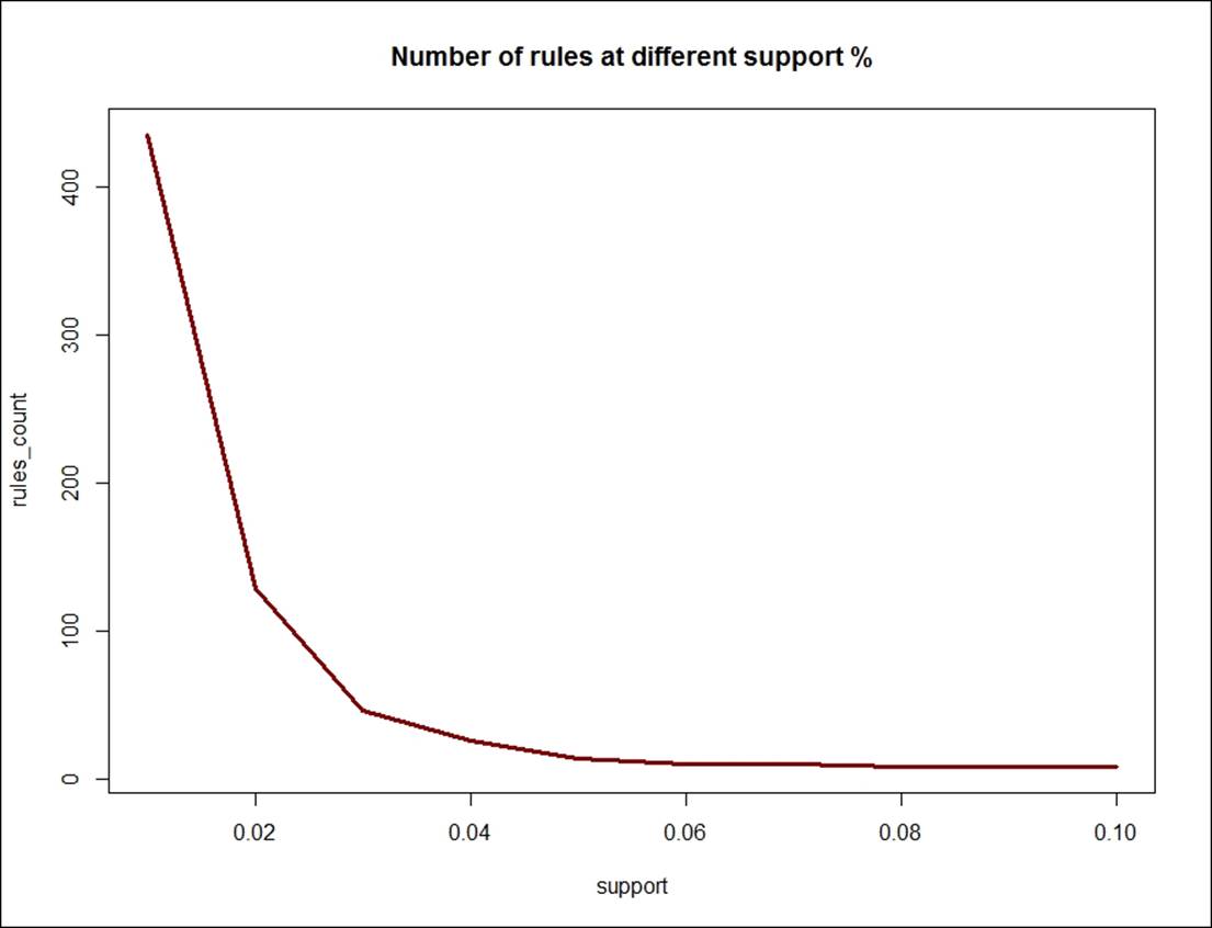
Looking at the support 0.04 and confidence level 10%, the right number of valid rules for the dataset would be 26, based on the scree-plot result. The reverse can happen too to identify relevant rules; keeping the support level constant and varying the confidence level, we can create another scree plot:

> conf<-seq(0.10,1.0,0.10)

> conf

[1] 0.1 0.2 0.3 0.4 0.5 0.6 0.7 0.8 0.9 1.0

> rules_count<-c(427,231,125,62,15,0,0,0,0,0)

> rules_count

[1] 427 231 125 62 15 0 0 0 0 0

> plot(conf,rules_count,type = "l",main="Number of rules at different confidence %",

+ col="darkred",lwd=3)

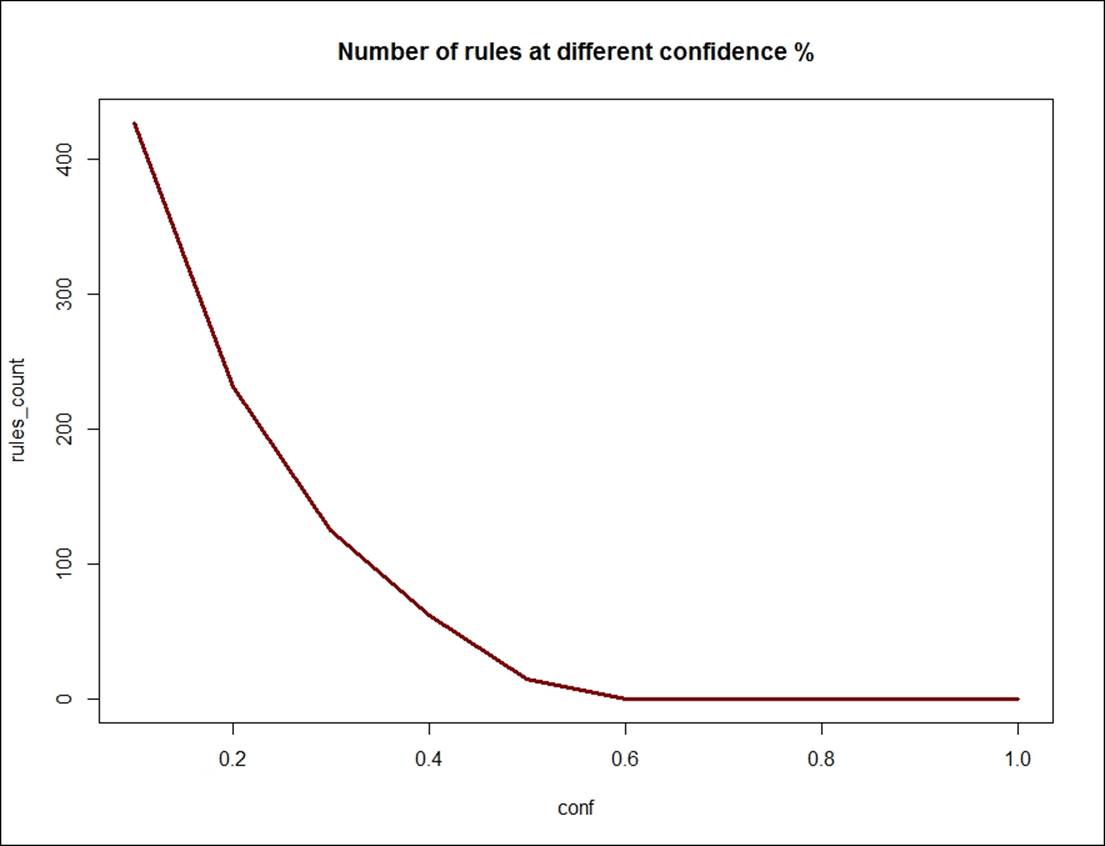
Looking at the confidence level of 0.5 and confidence level changing by 10%, the right number of valid rules for the groceries dataset would be 15, based on the scree plot result.

Eclat algorithm

Eclat algorithm uses simple intersection operations for homogenous class clustering with a bottom-up approach. The same code can be re-run using the eclat function in R and the result can be retrieved. The eclat function accepts two arguments, support and maximum length:

> rules_ec <- eclat(Groceries, parameter = list(supp = 0.05))

parameter specification:

tidLists support minlen maxlen target ext

FALSE 0.05 1 10 frequent itemsets FALSE

algorithmic control:

sparse sort verbose

7 -2 TRUE

eclat - find frequent item sets with the eclat algorithm

version 2.6 (2004.08.16) (c) 2002-2004 Christian Borgelt

create itemset ...

set transactions ...[169 item(s), 9835 transaction(s)] done [0.00s].

sorting and recoding items ... [28 item(s)] done [0.00s].

creating sparse bit matrix ... [28 row(s), 9835 column(s)] done [0.00s].

writing ... [31 set(s)] done [0.00s].

Creating S4 object ... done [0.00s].

> summary(rules_ec)

set of 31 itemsets

most frequent items:

whole milk other vegetables yogurt rolls/buns frankfurter

4 2 2 2 1

(Other)

23

element (itemset/transaction) length distribution:sizes

1 2

28 3

Min. 1st Qu. Median Mean 3rd Qu. Max.

1.000 1.000 1.000 1.097 1.000 2.000

summary of quality measures:

support

Min. :0.05236

1st Qu.:0.05831

Median :0.07565

Mean :0.09212

3rd Qu.:0.10173

Max. :0.25552

includes transaction ID lists: FALSE

mining info:

data ntransactions support

Groceries 9835 0.05

Using the eclat algorithm, with a support of 5%, there are 31 rules that explain the relationship between different items. The rule includes items that have a representation in at least 5% of the transactions.

While generating a product recommendation, it is important to recommend those rules that have high confidence level, irrespective of support proportion. Based on confidence, the top 5 rules can be derived as follows:

> #sorting out the most relevant rules

> rules<-sort(rules, by="confidence", decreasing=TRUE)

> inspect(rules[1:5])

lhs rhs support confidence lift

36 {other vegetables,yogurt} => {whole milk} 0.02226741 0.5128806 2.007235

10 {butter} => {whole milk} 0.02755465 0.4972477 1.946053

3 {curd} => {whole milk} 0.02613116 0.4904580 1.919481

33 {root vegetables,other vegetables} => {whole milk} 0.02318251 0.4892704 1.914833

34 {root vegetables,whole milk} => {other vegetables} 0.02318251 0.4740125 2.449770

Rules also can be sorted based on lift and support proportion, by changing the argument in the sort function. The top 5 rules based on lift calculation are as follows:

> rules<-sort(rules, by="lift", decreasing=TRUE)

> inspect(rules[1:5])

lhs rhs support confidence lift

35 {other vegetables,whole milk} => {root vegetables} 0.02318251 0.3097826 2.842082

34 {root vegetables,whole milk} => {other vegetables} 0.02318251 0.4740125 2.449770

27 {root vegetables} => {other vegetables} 0.04738180 0.4347015 2.246605

15 {whipped/sour cream} => {other vegetables} 0.02887646 0.4028369 2.081924

37 {whole milk,yogurt} => {other vegetables} 0.02226741 0.3974592 2.054131

Visualizing association rules

How the items are related and how the rules can be visually represented is as much important as creating the rules:

> #visualizign the rules

> plot(rules,method='graph',interactive = T,shading = T)

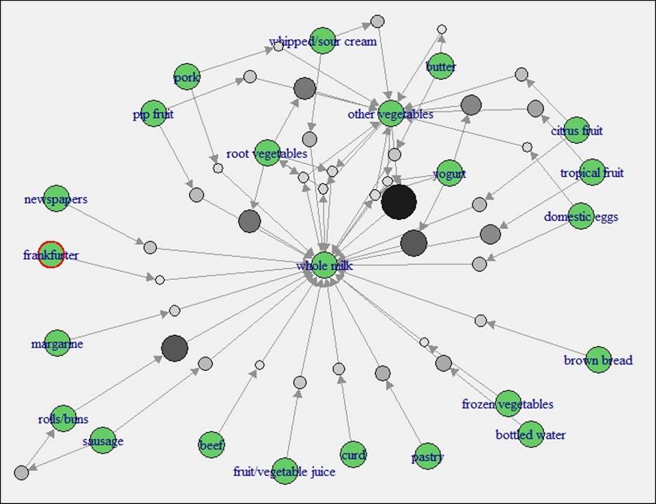
The preceding graph is created using apriori algorithm. In maximum number of rules, at least you would find either whole milk or other vegetables as those two items are well connected by nodes with other items.

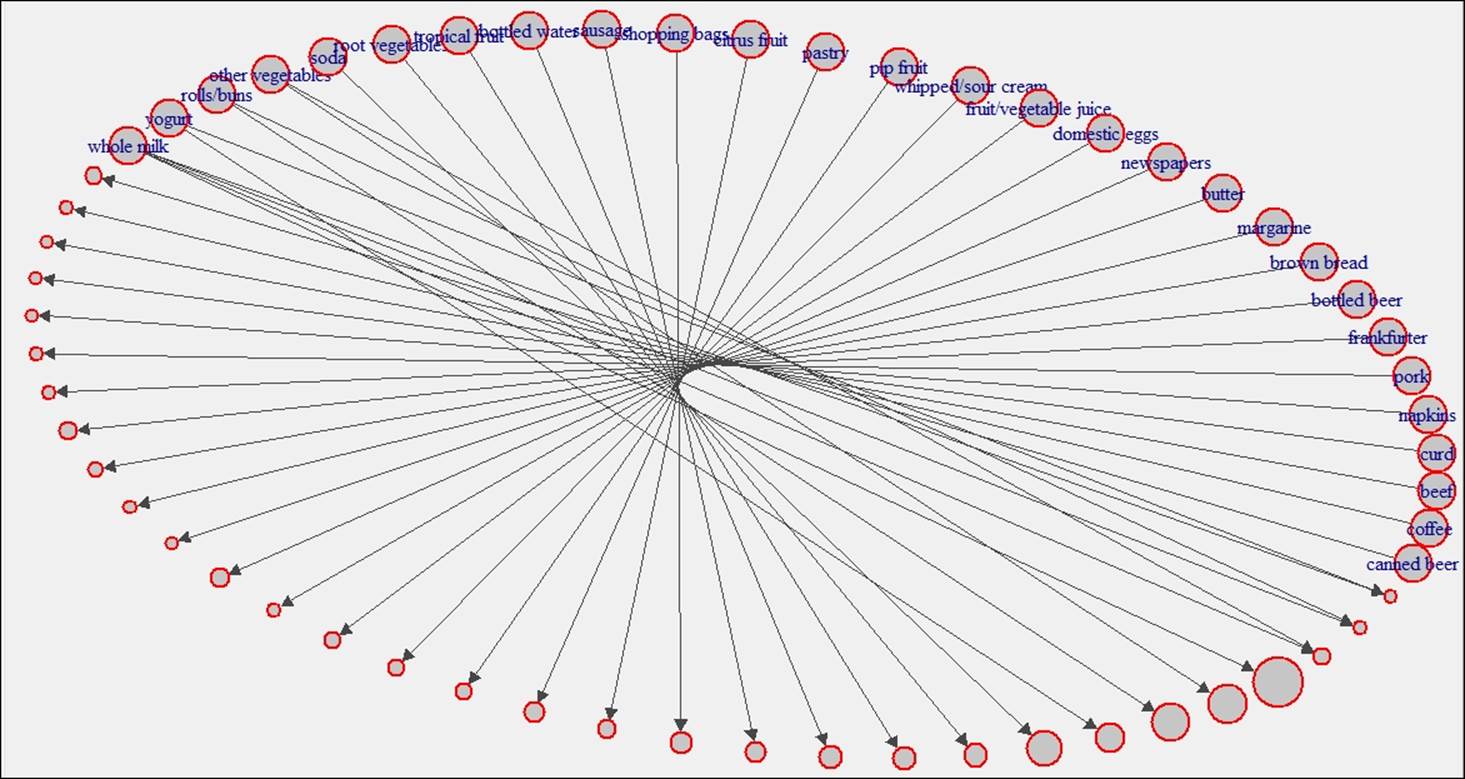
Using eclat algorithm for the same dataset, we have created another set of rules; the following graph shows the visualization of the rules:

Implementation of arules

Once a good market basket analysis or arules model is built, the next task is to integrate the model. arules provides a PMML interface, which is a predictive modeling markup language interface, to integrate with other applications. Other applications can be other statistical software such as, SAS, SPSS, and so on; or it can be Java, PHP, and Android-based applications. The PMML interface makes it easier to integrate the model. When it comes to rule implementation, two important questions a retailer would like to get answer are:

· What are customers likely to buy before buying a product?

· What are the customers likely to buy if they have already purchased some product?

Let's take a product yogurt, and the retailer would like to recommend this to customers. Which are the rules that can help the retailer? So the top 5 rules are as follows:

> rules<-apriori(data=Groceries, parameter=list(supp=0.001,conf = 0.8),

+ appearance = list(default="lhs",rhs="yogurt"),

+ control = list(verbose=F))

> rules<-sort(rules, decreasing=TRUE,by="confidence")

> inspect(rules[1:5])

lhs rhs support confidence

4 {root vegetables,butter,cream cheese } => {yogurt} 0.001016777 0.9090909

10 {tropical fruit,whole milk,butter,sliced cheese} => {yogurt} 0.001016777 0.9090909

11 {other vegetables,curd,whipped/sour cream,cream cheese } => {yogurt} 0.001016777 0.9090909

13 {tropical fruit,other vegetables,butter,white bread} => {yogurt} 0.001016777 0.9090909

2 {sausage,pip fruit,sliced cheese} => {yogurt} 0.001220132 0.8571429

lift

4 6.516698

10 6.516698

11 6.516698

13 6.516698

2 6.144315

> rules<-apriori(data=Groceries, parameter=list(supp=0.001,conf = 0.10,minlen=2),

+ appearance = list(default="rhs",lhs="yogurt"),

+ control = list(verbose=F))

> rules<-sort(rules, decreasing=TRUE,by="confidence")

> inspect(rules[1:5])

lhs rhs support confidence lift

20 {yogurt} => {whole milk} 0.05602440 0.4016035 1.571735

19 {yogurt} => {other vegetables} 0.04341637 0.3112245 1.608457

18 {yogurt} => {rolls/buns} 0.03436706 0.2463557 1.339363

15 {yogurt} => {tropical fruit} 0.02928317 0.2099125 2.000475

17 {yogurt} => {soda} 0.02735130 0.1960641 1.124368

Using the lift criteria also, product recommendation can be designed to offer to the customers:

> # sorting grocery rules by lift

> inspect(sort(rules, by = "lift")[1:5])

lhs rhs support confidence lift

1 {yogurt} => {curd} 0.01728521 0.1239067 2.325615

8 {yogurt} => {whipped/sour cream} 0.02074225 0.1486880 2.074251

15 {yogurt} => {tropical fruit} 0.02928317 0.2099125 2.000475

4 {yogurt} => {butter} 0.01464159 0.1049563 1.894027

11 {yogurt} => {citrus fruit} 0.02165735 0.1552478 1.875752

Finding out the subset of rules based on the availability of some item names can be done using the following code:

# finding subsets of rules containing any items

itemname_rules <- subset(rules, items %in% "item name")

inspect(itemname_rules[1:5])

> # writing the rules to a CSV file

> write(rules, file = "groceryrules.csv", sep = ",", quote = TRUE, row.names = FALSE)

>

> # converting the rule set to a data frame

> groceryrules_df <- as(rules, "data.frame")

Summary

In this chapter, we discussed how to create association rules, what all factors determine the rules' existence, and how rules explain the underlying relationship between different items or variables. Also we looked at how we can get most compressed rules based on minimum support and confidence value. The objective of the association rules model was not to come up with rules but to implement the rules in business use cases for generating recommendation for cross-selling and upselling products, and designing campaign bundles based on association. The rules would provide necessary guidance for the store managers to place products and merchandising design in a retail setup. Having said this, in our next chapter, we are going to cover various methods of performing clustering for segmentation, which would provide more insights into product recommendation using clustering methods.