R Data Mining Blueprints (2016)

Chapter 4. Regression with Automobile Data

One of the primary objectives of data mining projects is to understand the relationship between various variables and establish a cause and effect relationship between the variable of interest and other explanatory variables. In data mining projects, performing predictive analytics not only entails insights on hidden messages in datasets but also helps in making future decisions which might impact the business outcomes. In this chapter, the reader will get to know the basics of predictive analytics using regression methods, including various linear and nonlinear regression methods using R programming. The reader will be able to understand the theoretical background as well as get practical hands-on experience with all the regression methods using R programming language.

In this chapter, we will cover the following topics:

· Regression formulation

· Linear regression

· Logical regression

· Cubic regression

· Stepwise regression

· Penalized regression

Regression introduction

Regression methods help in predicting the future outcomes of a target variable. As an example, here are a few business cases:

· In the sales and marketing domain, how can a business achieve a significant improvement in sales? Can we successfully predict using the if a necessary amendment is made to the drivers of sales?

· In the retail domain, can we predict the number of visitors to a website, so that necessary tech support can be aligned to help operate the site better?

· How can a retail/e-commerce owner predict the number of footfall to their store in a month/week/year?

· In the banking domain, how can a bank predict the number of people applying for home loans, car loans, and personal loans, so that they can maintain their liquid capital to support the demand?

· In the banking domain, prediction of default probability can be estimated using regression methods so that a bank can decide whether to approve a loan/credit card to a customer.

· In the automobile manufacturing domain, the sales unit of vehicles is indirectly proportional to the price of the vehicles and the price of a vehicle is decided by many factors such as usages of different metals/components, and various vehicle features such as RPM, mileage, length, width, and others. How can a manufacturer predict the unit of sales?

There are different methods to perform regression, including both linear as well as non-linear. Regression-based predictive analytics is being used in different industries in a different way. Regression methods support the prediction of a continuous variable, prediction of the probability of a success or failure of a variable, prediction of events based on features, and so on.

Formulation of regression problem

The formulation of a regression problem is very essential in creating a good regression-based predictive model. A typical approach in building a good predictive model follows a process of converting a business problem to a statistical problem, then converting the statistical problem to a statistical solution, and finally converting the statistical solution to a business solution. The following steps are required to build a good predictive model using regression based methods:

· A clear understanding about the background or context is very much required. Sometimes a good predictive model does not make sense for a business from a context point of view. However, a contextually relevant predictive model may not be a good predictive model.

· A clear understanding about the objective is needed: what are you predicting and why are you predicting? Domain expertise is required. Most of the times, non-relevant features get added to a model, having no practical sense, because they show a mere correlation.

· A clear understanding about correlation and regression is important. It's a common phenomenon that people misconstrue a mere correlation or association as regression. "All regression may show causal relationship, but not the contrary".

· Conversion of a business problem to a statistical problem should be done carefully, so that assumptions and business understanding can be taken care of in the model.

Initial exploratory data analysis reveals the relationship between variables so that the variables can be included in a predictive model. The exploratory data analysis involves univariate, bivariate, and multivariate data analysis. Missing value imputation, outlier treatment, and removal of data entry errors are also equally important before proceeding with regression methods.

Case study

We are going to take two datasets, Cars93_1.csv and ArtPiece_2.csv, to explain various regression methods with a detailed analysis of what regression to use where and under what circumstances. For each regression method, we will take a look at the assumptions, limitations, mathematical formulations, and interpretation of the results.

Linear regression

The linear regression model is used for explaining the relationship between a single dependent variable known as Y and one or more X's independent variables known as input, predictor, or independent variables. The following two equations explain a linear regression scenario:

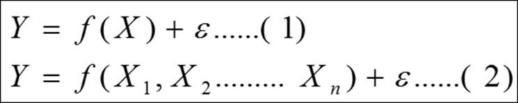
Equation 1 shows the formulation of a simple linear regression equation and equation 2 shows the multiple linear equations where many independent variables can be included. The dependent variable must be a continuous variable and the independent variables can be continuous and categorical. We are going to explain the multiple linear regression analysis by taking the Cars93_1.csv dataset, where the dependent variable is the price of cars and all the other variables are explanatory variables. The regression analysis includes:

· Predicting the future values of the dependent variable, given the values for independent variables

· Assessment of model fit statistics and comparison of various models

· Interpreting the coefficients to understand the levers of change in the dependent variable

· The relative importance of the independent variables

The primary objective of a regression model is to estimate the beta parameters and minimize the error term epsilon:

Let's look at the relationship between various variables using a correlation plot:

#Scatterplot showing all the variables in the dataset

library(car);attach(Cars93_1)

> #12-"Rear.seat.room",13-"Luggage.room" has NA values need to remove them

> m<-cor(Cars93_1[,-c(12,13)])

> corrplot(m, method = "ellipse")

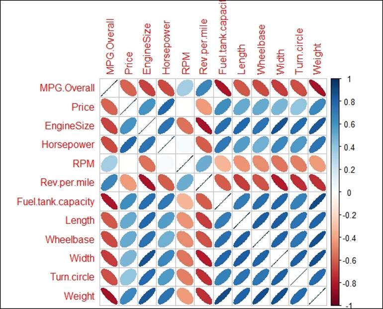
The preceding figure shows the relationship between various variables. From each ellipse we can get to know how the relationship: is it positive or negative, and is it strongly associated, moderately associated, or weakly associated? The correlation plot helps in taking a decision on which variables to keep for further investigation and which ones to remove from further analysis. The dark brown colored ellipse indicates perfect negative correlation and the dark blue colored ellipse indicates the perfect positive correlation. The narrower the ellipse, the higher the degree of correlation.

Given the number of variables in the dataset, it is quite difficult to read the scatterplot. Hence the correlation between all the variables can be represented using a correlation graph, as follows:

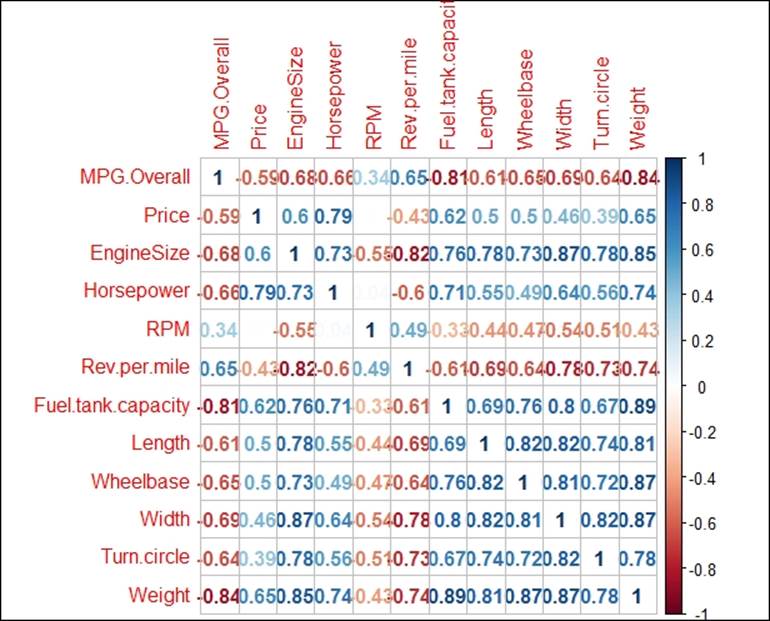
Correlation coefficients represented in bold blue color show higher degree of positive correlation and the ones with red color show higher degree of negative correlation.

The assumptions of a linear regression are as follows:

· Normality: The error terms from the estimated model should follow a normal distribution

· Linearity: The parameters to be estimated should be linear

· Independence: The error terms should be independent, hence no-autocorrelation

· Equal variance: The error terms should be homoscedastic

· Multicollinearity: The correlation between the independent variables should be zero or minimum

While fitting a multiple linear regression model, it is important to take care of the preceding assumptions. Let's look at the summary statistics from the multiple linear regression analysis and interpret the assumptions:

> #multiple linear regression model

> fit<-lm(MPG.Overall~.,data=Cars93_1)

> #model summary

> summary(fit)

Call:

lm(formula = MPG.Overall ~ ., data = Cars93_1)

Residuals:

Min 1Q Median 3Q Max

-5.0320 -1.4162 -0.0538 1.2921 9.8889

Coefficients:

Estimate Std. Error t value Pr(>|t|)

(Intercept) 2.808773 16.112577 0.174 0.86213

Price -0.053419 0.061540 -0.868 0.38842

EngineSize 1.334181 1.321805 1.009 0.31638

Horsepower 0.005006 0.024953 0.201 0.84160

RPM 0.001108 0.001215 0.912 0.36489

Rev.per.mile 0.002806 0.001249 2.247 0.02790 *

Fuel.tank.capacity -0.639270 0.262526 -2.435 0.01752 *

Length -0.059862 0.065583 -0.913 0.36459

Wheelbase 0.330572 0.156614 2.111 0.03847 *

Width 0.233123 0.265710 0.877 0.38338

Turn.circle 0.026695 0.197214 0.135 0.89273

Rear.seat.room -0.031404 0.182166 -0.172 0.86364

Luggage.room 0.206758 0.188448 1.097 0.27644

Weight -0.008001 0.002849 -2.809 0.00648 **

---

Signif. codes: 0 '***' 0.001 '**' 0.01 '*' 0.05 '.' 0.1 ' ' 1

Residual standard error: 2.835 on 68 degrees of freedom

(11 observations deleted due to missingness)

Multiple R-squared: 0.7533, Adjusted R-squared: 0.7062

F-statistic: 15.98 on 13 and 68 DF, p-value: 7.201e-16

In the previous multiple linear regression model using all the independent variables, we are predicting the mileage per gallon MPG.Overall variable. From the model summary, it is observed that few independent variables are statistically significant at 95% confidence level. The coefficient of determination R² which is known as the goodness of fit of a regression model is 75.33%. This implies that 75.33% variation in the dependent variable is explained by all the independent variables together. The formula for computing multiple R² is given next:

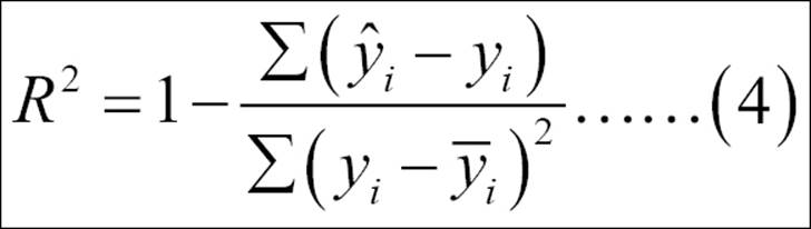
The preceding equation 4 calculated the coefficient of determination or percentage of variance explained by the regression model. The base line score to qualify for a good regression model is at least 80% as R square value; any R square value more than 80% is considered to be very good regression model. Since the R² is now less than 80%, we need to perform a few diagnostic tests on the regression results.

The estimated beta coefficients of the model:

> #estimated coefficients

> fit$coefficients

(Intercept) Price EngineSize Horsepower

2.808772930 -0.053419142 1.334180881 0.005005690

RPM Rev.per.mile Fuel.tank.capacity Length

0.001107897 0.002806093 -0.639270186 -0.059861997

Wheelbase Width Turn.circle Rear.seat.room

0.330572119 0.233123382 0.026694571 -0.031404262

Luggage.room Weight

0.206757968 -0.008001444

#residual values

fit$residuals

#fitted values from the model

fit$fitted.values

#what happened to NA

fit$na.action

> #ANOVA table from the model

> summary.aov(fit)

Df Sum Sq Mean Sq F value Pr(>F)

Price 1 885.7 885.7 110.224 7.20e-16 ***

EngineSize 1 369.3 369.3 45.959 3.54e-09 ***

Horsepower 1 37.4 37.4 4.656 0.03449 *

RPM 1 38.8 38.8 4.827 0.03143 *

Rev.per.mile 1 71.3 71.3 8.877 0.00400 **

Fuel.tank.capacity 1 147.0 147.0 18.295 6.05e-05 ***

Length 1 1.6 1.6 0.203 0.65392

Wheelbase 1 35.0 35.0 4.354 0.04066 *

Width 1 9.1 9.1 1.139 0.28969

Turn.circle 1 0.5 0.5 0.060 0.80774

Rear.seat.room 1 0.6 0.6 0.071 0.79032

Luggage.room 1 9.1 9.1 1.129 0.29170

Weight 1 63.4 63.4 7.890 0.00648 **

Residuals 68 546.4 8.0

---

Signif. codes: 0 '***' 0.001 '**' 0.01 '*' 0.05 '.' 0.1 ' ' 1

11 observations deleted due to missingness

From the preceding analysis of variance (ANOVA) table, it is observed that the variables Length, Width, turn circle, rear seat room, and luggage room are not statistically significant at 5% level of alpha. ANOVA shows the source of variation in dependent variable from any independent variable. It is important to apply ANOVA after the regression model to know which independent variable has significant contribution to the dependent variable:

> #visualizing the model statistics

> par(mfrow=c(1,2))

> plot(fit, col="dodgerblue4")

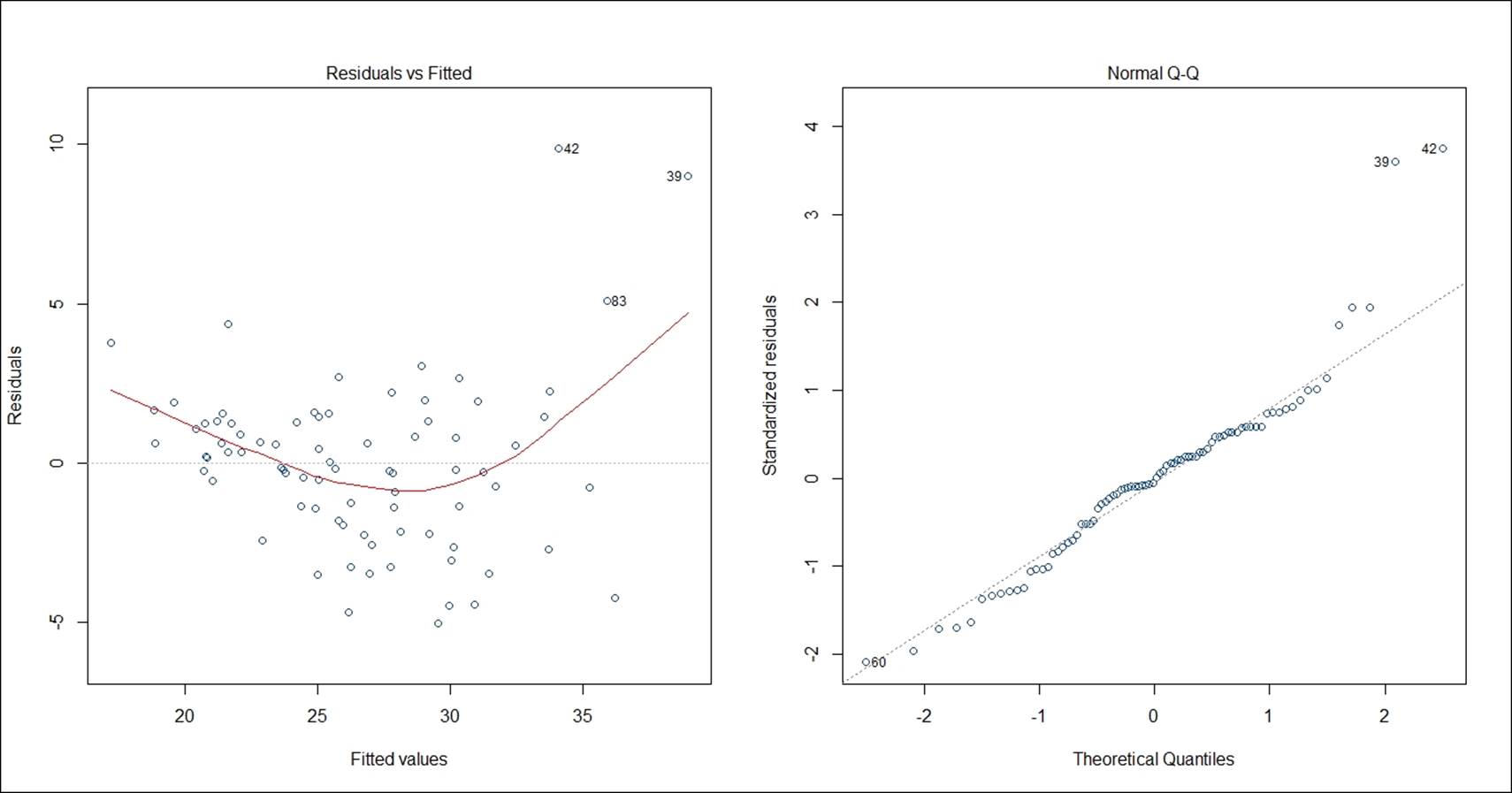
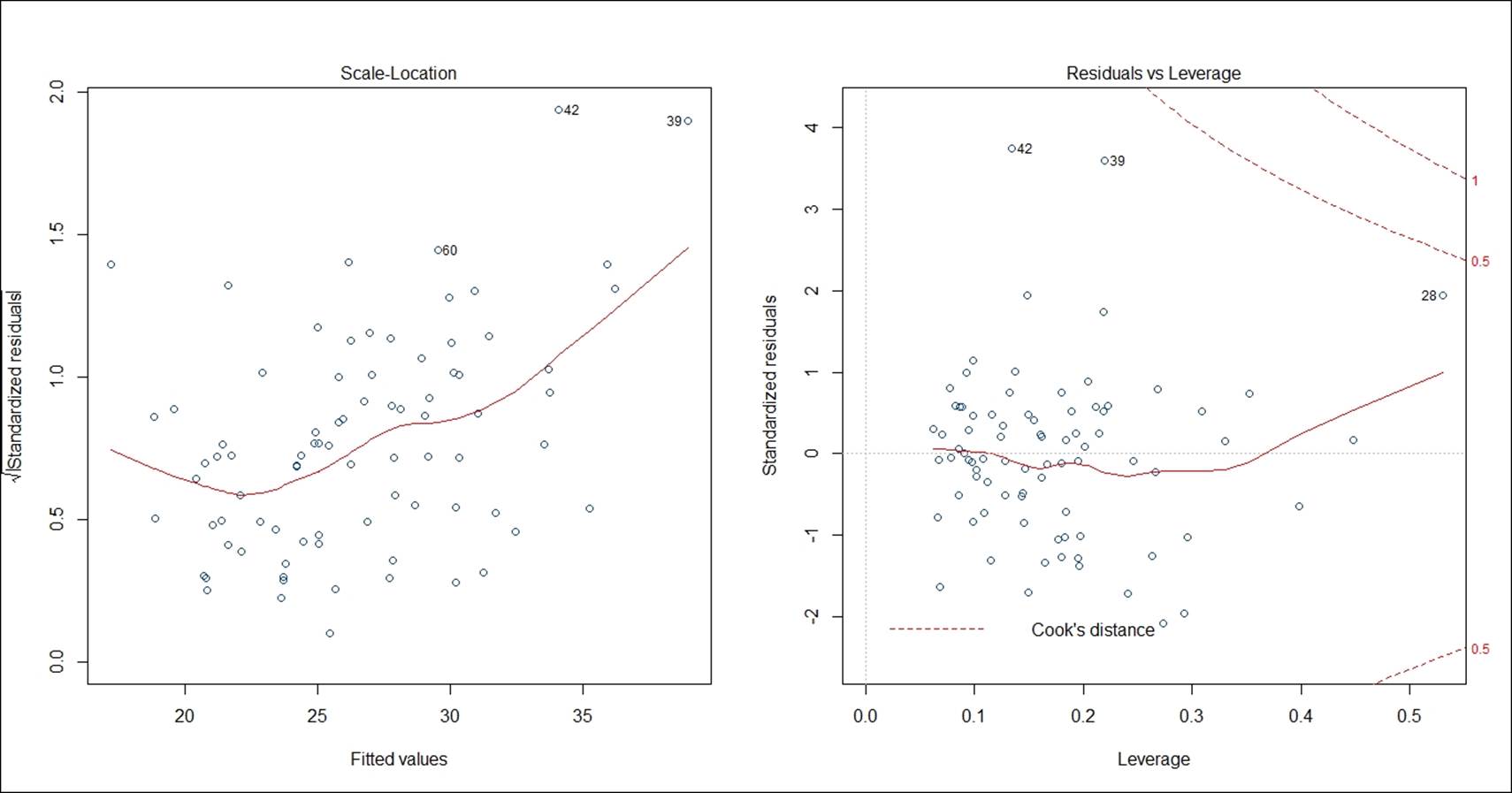
The residual versus fitted plot shows the randomness in residual values as we move along the fitted line. If the residual values display any pattern against the fitted values, the error term is not probably normal. The residual versus fitted graph indicates that there is no pattern that exists among the residual terms; the residuals are approximately normally distributed. Residual is basically that part of the model which cannot be explained by the model. There are few influential data points, for example, 42^nd, 39^th, and 83^rd as it is shown on the preceding graph, the normal quantile-quantile plot indicates except few influential data points all other standardized residual points follow a normal distribution. The straight line is the zero residual line and the red line is the pattern of residual versus fitted relationship. The scale versus location graph and the residuals versus leverage graph also validate the same observation that the residual term has no trend. The scale versus location plot takes the square root of the standardized residuals and plots it against the fitted values:

The confidence interval of the model coefficients at 95% confidence level can be calculated using the following code and also the prediction interval at 95% confidence level for all the fitted values can be calculated using the code below. The formula to compute the confidence interval is the model coefficient +/- standard error of model coefficient * 1.96:

> confint(fit,level=0.95)

2.5 % 97.5 %

(Intercept) -2.934337e+01 34.960919557

Price -1.762194e-01 0.069381145

EngineSize -1.303440e+00 3.971801771

Horsepower -4.478638e-02 0.054797758

RPM -1.315704e-03 0.003531499

Rev.per.mile 3.139667e-04 0.005298219

Fuel.tank.capacity -1.163133e+00 -0.115407347

Length -1.907309e-01 0.071006918

Wheelbase 1.805364e-02 0.643090600

Width -2.970928e-01 0.763339610

Turn.circle -3.668396e-01 0.420228772

Rear.seat.room -3.949108e-01 0.332102243

Luggage.room -1.692837e-01 0.582799642

Weight -1.368565e-02 -0.002317240

> head(predict(fit,interval="predict"))

fit lwr upr

1 31.47382 25.50148 37.44615

2 24.99014 18.80499 31.17528

3 22.09920 16.09776 28.10064

4 21.19989 14.95606 27.44371

5 21.62425 15.37929 27.86920

6 27.89137 21.99947 33.78328

The existence of influential data points or outlier values may deviate the model result, hence identification and curation of outlier data points in the regression model is very important:

# Deletion Diagnostics

influence.measures(fit)

The function belongs to the stats library, which computes some of the regression diagnostics for linear and generalized models. Any observation labeled with a star (*) implies an influential data point, that can be removed to make the model good:

# Index Plots of the influence measures

influenceIndexPlot(fit, id.n=3)

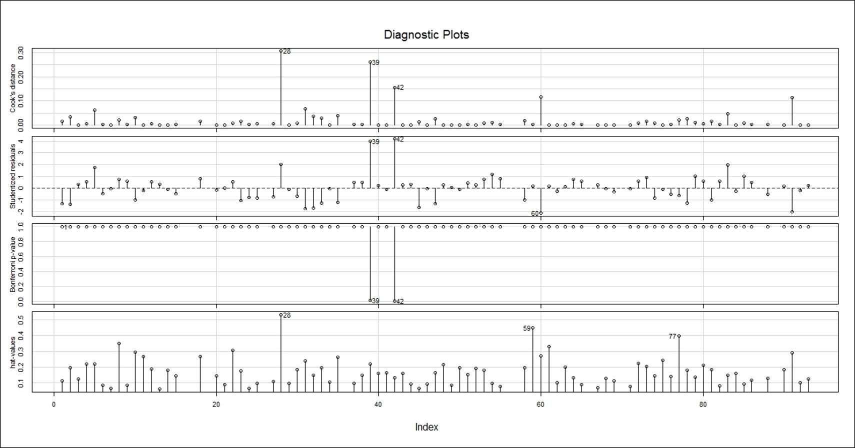
The influential data points are highlighted by their position in the dataset. In order to understand more about these influential data points, we can write the following command. The size of the red circle based on the cook's distance value indicates the order of influence. Cook's distance is a statistical method to identify data points which have more influence than other data points.

Generally, these are data points that are distant from other points in the data, either for the dependent variable or one or more independent variables:

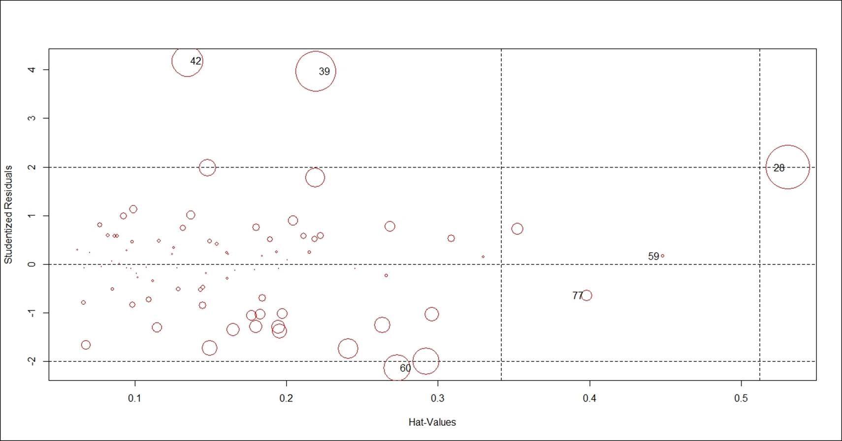
> # A user friendly representation of the above

> influencePlot(fit,id.n=3, col="red")

StudRes Hat CookD

28 1.9902054 0.5308467 0.55386748

39 3.9711522 0.2193583 0.50994280

42 4.1792327 0.1344866 0.39504695

59 0.1676009 0.4481441 0.04065691

60 -2.1358078 0.2730012 0.34097909

77 -0.6448891 0.3980043 0.14074778

If we remove these influential data points from our model, we can see some improvement in the model goodness of fit and overall error for the model can be reduced. Removing all the influential points at one go is not a good idea; hence we will take a step-by-step approach to deleting these influential data points from the model and monitor the improvement in the model statistics:

> ## Regression after deleting the 28th observation

> fit.1<-lm(MPG.Overall~., data=Cars93_1[-28,])

> summary(fit.1)

Call:

lm(formula = MPG.Overall ~ ., data = Cars93_1[-28, ])

Residuals:

Min 1Q Median 3Q Max

-5.0996 -1.7005 0.4617 1.4478 9.4168

Coefficients:

Estimate Std. Error t value Pr(>|t|)

(Intercept) -6.314222 16.425437 -0.384 0.70189

Price -0.014859 0.063281 -0.235 0.81507

EngineSize 2.395780 1.399569 1.712 0.09156 .

Horsepower -0.022454 0.028054 -0.800 0.42632

RPM 0.001944 0.001261 1.542 0.12789

Rev.per.mile 0.002829 0.001223 2.314 0.02377 *

Fuel.tank.capacity -0.640970 0.256992 -2.494 0.01510 *

Length -0.065310 0.064259 -1.016 0.31311

Wheelbase 0.407332 0.158089 2.577 0.01219 *

Width 0.204212 0.260513 0.784 0.43587

Turn.circle 0.071081 0.194340 0.366 0.71570

Rear.seat.room -0.004821 0.178824 -0.027 0.97857

Luggage.room 0.156403 0.186201 0.840 0.40391

Weight -0.008597 0.002804 -3.065 0.00313 **

---

Signif. codes: 0 '***' 0.001 '**' 0.01 '*' 0.05 '.' 0.1 ' ' 1

Residual standard error: 2.775 on 67 degrees of freedom

(11 observations deleted due to missingness)

Multiple R-squared: 0.7638, Adjusted R-squared: 0.718

F-statistic: 16.67 on 13 and 67 DF, p-value: 3.39e-16

Regression output after deleting the most influential data point provides a significant improvement in the R2 value from 75.33% to 76.38%. Let's repeat the same activity and see the model's results:

> ## Regression after deleting the 28,39,42,59,60,77 observations

> fit.2<-lm(MPG.Overall~., data=Cars93_1[-c(28,42,39,59,60,77),])

> summary(fit.2)

Call:

lm(formula = MPG.Overall ~ ., data = Cars93_1[-c(28, 42, 39,

59, 60, 77), ])

Residuals:

Min 1Q Median 3Q Max

-3.8184 -1.3169 0.0085 0.9407 6.3384

Coefficients:

Estimate Std. Error t value Pr(>|t|)

(Intercept) 21.4720002 13.3375954 1.610 0.11250

Price -0.0459532 0.0589715 -0.779 0.43880

EngineSize 2.4634476 1.0830666 2.275 0.02641 *

Horsepower -0.0313871 0.0219552 -1.430 0.15785

RPM 0.0022055 0.0009752 2.262 0.02724 *

Rev.per.mile 0.0016982 0.0009640 1.762 0.08307 .

Fuel.tank.capacity -0.6566896 0.1978878 -3.318 0.00152 **

Length -0.0097944 0.0613705 -0.160 0.87372

Wheelbase 0.2298491 0.1288280 1.784 0.07929 .

Width -0.0877751 0.2081909 -0.422 0.67477

Turn.circle 0.0347603 0.1513314 0.230 0.81908

Rear.seat.room -0.2869723 0.1466918 -1.956 0.05494 .

Luggage.room 0.1828483 0.1427936 1.281 0.20514

Weight -0.0044714 0.0021914 -2.040 0.04557 *

---

Signif. codes: 0 '***' 0.001 '**' 0.01 '*' 0.05 '.' 0.1 ' ' 1

Residual standard error: 2.073 on 62 degrees of freedom

(11 observations deleted due to missingness)

Multiple R-squared: 0.8065, Adjusted R-squared: 0.7659

F-statistic: 19.88 on 13 and 62 DF, p-value: < 2.2e-16

Looking at the preceding output, we can conclude that the removal of outliers or influential data points adds robustness to the R-square value. Now we can conclude that 80.65% of the variation in the dependent variable is being explained by all the independent variables in the model.

Now, using studentised residuals against t-quantiles in a Q-Q plot, we can identify some more outliers data points, if any, to boost the model accuracy:

> # QQ plots of studentized residuals, helps identify outliers

> qqPlot(fit.2, id.n=5)

91 32 55 5 83

1 2 74 75 76

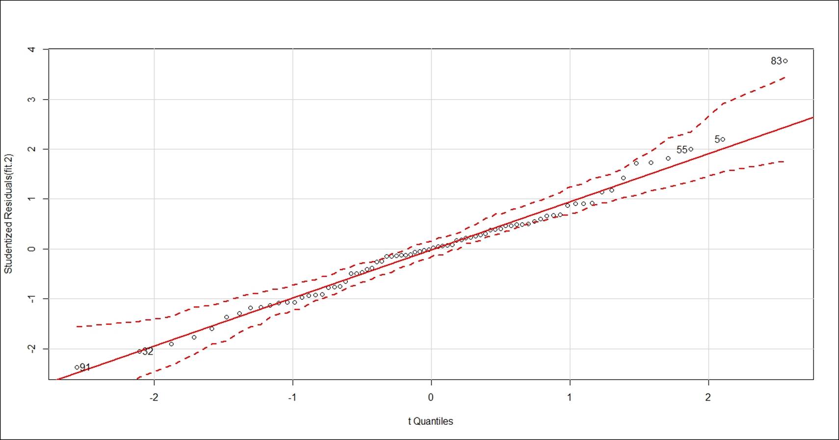
From the preceding Q-Q plot, it seems that the data is fairly normally distributed, except few outlier values such as 83^rd, 91^st, 32^nd, 55^th, and 5^th data points:

> ## Diagnostic Plots ###

> influenceIndexPlot(fit.2, id.n=3)

> influencePlot(fit.2, id.n=3, col="blue")

StudRes Hat CookD

5 2.1986298 0.2258133 0.30797166

8 -0.1448259 0.4156467 0.03290507

10 -0.7655338 0.3434515 0.14847534

83 3.7650470 0.2005160 0.45764995

91 -2.3672942 0.3497672 0.44770173

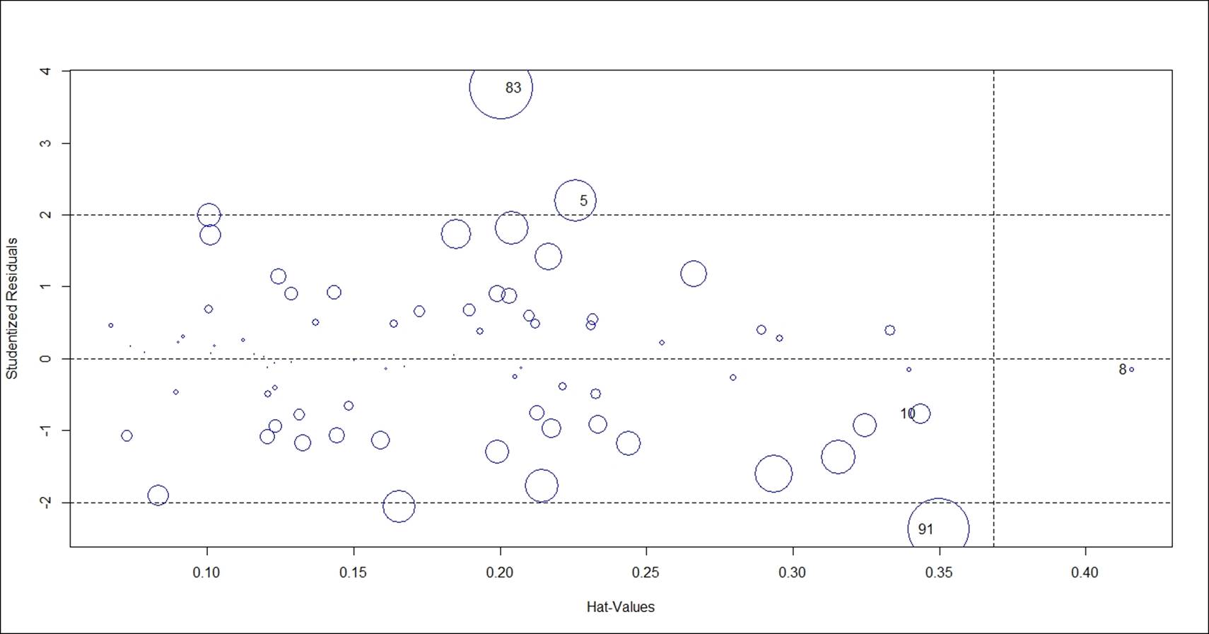
The problem of multicollinearity, that is, the correlation between predictor variables, needs to be verified for the final regression model. Variance Inflation Factor (VIF) is the measure typically used to estimate the multicollinearity. The formula to compute the VIF is 1/ (1-R² ). Any independent variable having a VIF value of more than 10 indicates multicollinearity; hence such variables need to be removed from the model. Deleting one variable at a time and then again checking the VIF for the model is the best way to do this:

> ### Variance Inflation Factors

> vif(fit.2)

Price EngineSize Horsepower RPM

4.799678 20.450596 18.872498 5.788160

Rev.per.mile Fuel.tank.capacity Length Wheelbase

3.736889 5.805824 15.200301 11.850645

Width Turn.circle Rear.seat.room Luggage.room

10.243223 4.006895 2.566413 2.935853

Weight

24.977015

Variable weight has the maximum VIF, hence deleting the variable make sense. After removing the variable, let's rerun the model and calculate the VIF:

## Regression after deleting the weight variable

fit.3<-lm(MPG.Overall~ Price+EngineSize+Horsepower+RPM+Rev.per.mile+

Fuel.tank.capacity+Length+Wheelbase+Width+Turn.circle+

Rear.seat.room+Luggage.room, data=Cars93_1[-c(28,42,39,59,60,77),])

summary(fit.3)

> vif(fit.3)

Price EngineSize Horsepower RPM

4.575792 20.337181 15.962349 5.372388

Rev.per.mile Fuel.tank.capacity Length Wheelbase

3.514992 4.863944 14.574352 11.013850

Width Turn.circle Rear.seat.room Luggage.room

10.240036 3.965132 2.561947 2.935690

## Regression after deleting the Enginesize variable

fit.4<-lm(MPG.Overall~ Price+Horsepower+RPM+Rev.per.mile+

Fuel.tank.capacity+Length+Wheelbase+Width+Turn.circle+

Rear.seat.room+Luggage.room, data=Cars93_1[-c(28,42,39,59,60,77),])

summary(fit.4)

vif(fit.4)

## Regression after deleting the Length variable

fit.5<-lm(MPG.Overall~ Price+Horsepower+RPM+Rev.per.mile+

Fuel.tank.capacity+Wheelbase+Width+Turn.circle+

Rear.seat.room+Luggage.room, data=Cars93_1[-c(28,42,39,59,60,77),])

summary(fit.5)

> vif(fit.5)

Price Horsepower RPM Rev.per.mile

4.419799 8.099750 2.595250 3.232048

Fuel.tank.capacity Wheelbase Width Turn.circle

4.679088 8.231261 7.953452 3.357780

Rear.seat.room Luggage.room

2.393630 2.894959

The coefficients from the final regression model:

> coefficients(fit.5)

(Intercept) Price Horsepower RPM

29.029107454 -0.089498236 -0.014248077 0.001071072

Rev.per.mile Fuel.tank.capacity Wheelbase Width

0.001591582 -0.769447316 0.130876817 -0.047053999

Turn.circle Rear.seat.room Luggage.room

-0.072030390 -0.240332275 0.216155256

Now we can conclude that there is no multicollinearity in the preceding regression model. We can write the final multiple linear regression equation as follows:

The estimated model parameters can be interpreted as, for one unit change in the price variable, the MPG overall is predicted to change by 0.09 unit. Likewise, the estimated model coefficients can be interpreted for all the other independent variables. If we know the values of these independent variables, we can predict the likely value of the dependent variable MPG overall by using the previous equation.

Stepwise regression method for variable selection

In stepwise regression method, a base regression model is formed using the OLS estimation method. Thereafter, a variable is added or subtracted to/from the base model depending upon the Akaike Information Criteria (AIC) value. The standard rule is that a minimum AIC would guarantee a best fit in comparison to other methods. Taking the Cars93_1.csv file, let's create a multiple linear regression model by using the stepwise method. There are three different ways to test out the best model using the step formula:

· Forward method

· Backward method

· Both

In the forward selection method, initially a null model is created and variable is added to see any improvement in the AIC value. The independent variables is added to the null model till there is an improvement in the AIC value. In backward selection method, the complete model is considered to be the base model. An independent variable is deducted from the model and the AIC value is checked. If there is an improvement in AIC, the variable would be removed; the process will go on till the AIC value becomes minimum. In both the methods, alternatively forward and back selection method is used to identify the most relevant model. Let's look at the model result at first iteration:

> #base model

> fit<-lm(MPG.Overall~.,data=Cars93_1)

> #stepwise regression

> model<-step(fit,method="both")

Start: AIC=183.52

MPG.Overall ~ Price + EngineSize + Horsepower + RPM + Rev.per.mile +

Fuel.tank.capacity + Length + Wheelbase + Width + Turn.circle +

Rear.seat.room + Luggage.room + Weight

Df Sum of Sq RSS AIC

- Turn.circle 1 0.147 546.54 181.54

- Rear.seat.room 1 0.239 546.64 181.56

- Horsepower 1 0.323 546.72 181.57

- Price 1 6.055 552.45 182.43

- Width 1 6.185 552.58 182.45

- RPM 1 6.686 553.08 182.52

- Length 1 6.695 553.09 182.52

- EngineSize 1 8.186 554.58 182.74

- Luggage.room 1 9.673 556.07 182.96

<none> 546.40 183.52

- Wheelbase 1 35.799 582.20 186.73

- Rev.per.mile 1 40.565 586.96 187.40

- Fuel.tank.capacity 1 47.646 594.04 188.38

- Weight 1 63.400 609.80 190.53

In the beginning, AIC is 183.52. In the final model, AIC is 175.51 and there are six independent variables, as shown next:

Step: AIC=175.51

MPG.Overall ~ EngineSize + RPM + Rev.per.mile + Fuel.tank.capacity +

Wheelbase + Width + Luggage.room + Weight

Df Sum of Sq RSS AIC

- Luggage.room 1 8.976 568.78 174.82

- Width 1 12.654 572.46 175.34

<none> 559.81 175.51

- EngineSize 1 14.022 573.83 175.54

- RPM 1 19.422 579.23 176.31

- Wheelbase 1 28.477 588.28 177.58

- Rev.per.mile 1 37.873 597.68 178.88

- Fuel.tank.capacity 1 52.516 612.32 180.86

- Weight 1 135.462 695.27 191.28

In the preceding table, "none" entry denotes the stage which is the final model, where further tuning or variable reduction is not possible. Hence, dropping more variables after that point would not make sense.

Logistic regression

The linear regression model based on the ordinary least square method assumes that the relationship between the dependent variable and the independent variables is linear; however, the logistic regression model assumes the relationship to be logarithmic. There are many real-life scenarios where the variable of interest is categorical in nature, such as buying a product or not, approving a credit card or not, tumor is cancerous or not, and so on. Logistic regression not only predicts a dependent variable class but it predicts the probability of a case belonging to a level in the dependent variable. The independent variables need not be normally distributed and need not have equal variance. Logistic regression belongs to the family of generalized linear regression. If the dependent variable has two levels then logistic regression can be applied, but if it has more than two levels, such as high, medium, and low, then multinomial logistic regression model can be applied. All the independent variables can be continuous, categorical, or nominal.

The logistic regression model can be explained using the following equation:

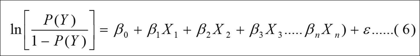
Ln (P(Y)/1-P(Y) ) is the log odds of the outcome. The beta coefficients mentioned in the previous equation explain how the log odds of the outcome variable increase or decrease for every one unit increase or decrease in the explanatory variable.

Let's take the Artpiece.csv dataset where the dependent variable is a good purchase or not need to be predicted based on the independent variables.

For a logistic regression model, the dependent variable needs to be a binary variable with two levels. If it is not then the first task is to convert the dependent variable to binary. For the independent variables it is important to check the type of the variable as well as the levels. If some independent variables are categorical then binary conversion (creating dummy variables for each category) is required. So here you go with data conversion in necessary format for the logistic regression model:

> #data conversion

> Artpiece$IsGood.Purchase<-as.factor(Artpiece$IsGood.Purchase)

> Artpiece$Is.It.Online.Sale<-as.factor(Artpiece$Is.It.Online.Sale)

> #removing NA, Missing values from the data

> Artpiece<-na.omit(Artpiece)

> ## 75% of the sample size

> smp_size <- floor(0.75 * nrow(Artpiece))

> ## set the seed to make your partition reproductible

> set.seed(123)

> train_ind <- sample(seq_len(nrow(Artpiece)), size = smp_size)

> train <- Artpiece[train_ind, ]

> test <- Artpiece[-train_ind, ]

The train dataset is used for building the logistic regression model and the test dataset would be used for testing the model:

> #Logistic regression Model

> model1<-glm(IsGood.Purchase ~.,family=binomial(logit),data=train)

> #Model results/ components

> summary(model1)

Call:

glm(formula = IsGood.Purchase ~ ., family = binomial(logit),

data = train)

Deviance Residuals:

Min 1Q Median 3Q Max

-2.1596 -0.4849 -0.4096 -0.3401 3.8760

Coefficients:

Estimate Std. Error z value Pr(>|z|)

(Intercept) -6.734e-01 1.250e+00 -0.539 0.58995

Critic.Ratings 1.372e-01 1.119e-02 12.267 < 2e-16 ***

Acq.Cost -7.998e-06 1.867e-06 -4.284 1.83e-05 ***

CurrentAuctionAveragePrice -1.460e-05 1.360e-06 -10.731 < 2e-16 ***

Brush.Size1 -1.378e+00 1.246e+00 -1.107 0.26840

Brush.Size2 -1.684e+00 1.246e+00 -1.352 0.17647

Brush.Size3 -1.128e+00 1.252e+00 -0.902 0.36730

Brush.SizeNULL 1.599e+00 1.246e+00 1.283 0.19946

CollectorsAverageprice -2.420e-05 4.677e-06 -5.175 2.28e-07 ***

Is.It.Online.Sale1 -1.710e-01 9.621e-02 -1.777 0.07552 .

Min.Guarantee.Cost 9.830e-06 3.329e-06 2.953 0.00314 **

---

Signif. codes: 0 '***' 0.001 '**' 0.01 '*' 0.05 '.' 0.1 ' ' 1

(Dispersion parameter for binomial family taken to be 1)

Null deviance: 40601 on 54500 degrees of freedom

Residual deviance: 34872 on 54490 degrees of freedom

AIC: 34894

Number of Fisher Scoring iterations: 5

From the previous model result, all the independent variables are statistically significant at 5% level except the brush variable, which is a categorical variable. The model automatically creates dummy variables for each of the levels of a categorical variable. It takes the first level from the categorical variable and compares with other level, if the row belongs to that category then 1 else 0. 95% confidence interval for model coefficients and exponentiated model coefficients can be calculated using the following script. The left hand side equation contains natural logarithm to remove that we have to make exponentiation of the right hand side expression which is the model coefficient:

> # 95% CI for exponentiated coefficients

> exp(confint(model1))

Waiting for profiling to be done...

2.5 % 97.5 %

(Intercept) 0.02301865 5.5660594

Critic.Ratings 1.12226719 1.1725835

Acq.Cost 0.99998833 0.9999957

CurrentAuctionAveragePrice 0.99998274 0.9999881

Brush.Size1 0.02326462 5.5558138

Brush.Size2 0.01714345 4.0948557

Brush.Size3 0.02953703 7.1850301

Brush.SizeNULL 0.45631813 109.1655370

CollectorsAverageprice 0.99996666 0.9999850

Is.It.Online.Sale1 0.69545357 1.0142229

Min.Guarantee.Cost 1.00000327 1.0000163

> confint(model1)

2.5 % 97.5 %

(Intercept) -3.771450e+00 1.716687e+00

Critic.Ratings 1.153509e-01 1.592094e-01

Acq.Cost -1.166650e-05 -4.348562e-06

CurrentAuctionAveragePrice -1.726348e-05 -1.193180e-05

Brush.Size1 -3.760822e+00 1.714845e+00

Brush.Size2 -4.066139e+00 1.409731e+00

Brush.Size3 -3.522110e+00 1.972000e+00

Brush.SizeNULL -7.845651e-01 4.692865e+00

CollectorsAverageprice -3.333576e-05 -1.500118e-05

Is.It.Online.Sale1 -3.631910e-01 1.412267e-02

Min.Guarantee.Cost 3.268054e-06 1.631710e-05

ANOVA can be performed on the results of the logistic regression model using chi-square test statistics. From the ANOVA which shows analysis of deviance in case of a logistic regression here, we can conclude that the deviance of model change is statistically significant when we include more independent variables in the model. The independent variables are added sequentially to the model and at every iteration the deviance of the error term is compared with the previous iteration to see if the addition or deletion of any variable is useful in reducing the error for the model:

> #ANOVA

> anova(model1,test="Chisq")

Analysis of Deviance Table

Model: binomial, link: logit

Response: IsGood.Purchase

Terms added sequentially (first to last)

Df Deviance Resid. Df Resid. Dev Pr(>Chi)

NULL 54500 40601

Critic.Ratings 1 354.6 54499 40246 < 2.2e-16 ***

Acq.Cost 1 477.8 54498 39768 < 2.2e-16 ***

CurrentAuctionAveragePrice 1 166.4 54497 39602 < 2.2e-16 ***

Brush.Size 4 4690.9 54493 34911 < 2.2e-16 ***

CollectorsAverageprice 1 27.3 54492 34884 1.773e-07 ***

Is.It.Online.Sale 1 3.3 54491 34880 0.067877 .

Min.Guarantee.Cost 1 8.6 54490 34872 0.003417 **

---

Signif. codes: 0 '***' 0.001 '**' 0.01 '*' 0.05 '.' 0.1 ' ' 1

>

> #Plotting the model

> plot(model1$fitted)

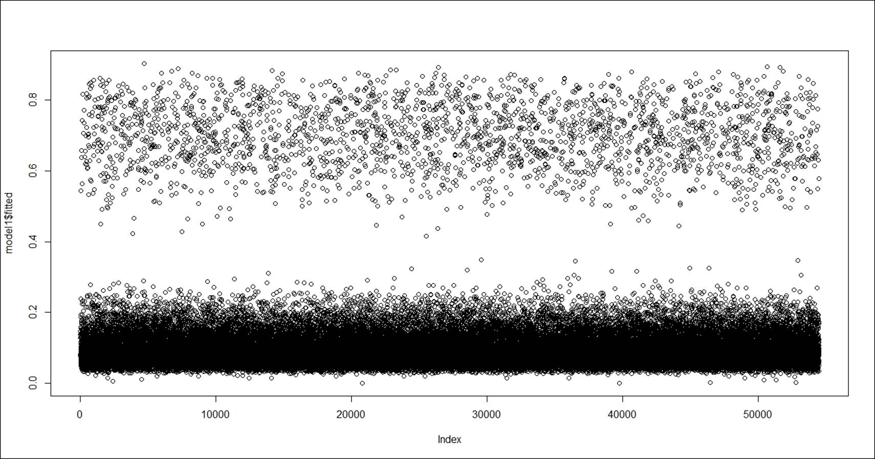
The preceding plot displays the fitted versus actual values (index) in a regression model. The predicted probability from the model can be extracted using the link option and the class prediction can be extracted using the response option, using the predictfunction:

> #Predicted Probability

> test$goodP<-predict(model1,newdata=test,type="response")

> test$goodL<-predict(model1,newdata=test,type="link")

Automatic logistic regression model selection can be done in three different ways using the stepwise regression method via AIC criteria:

· Backward selection method: All the independent variables are part of the initial model. Using Wald chi-square test of significance, variables with lowest value of chi-square or highest p-value such that it exceeds 0.05 (given that 95% confidence interval is used in the model) are removed from the model. The backward selection process of variable removal stops when it is not possible to find a variable that fits the Wald test criteria.

· Forward selection method: Model starts with a null model. A variable is entered into the model based on the lowest p-value or highest chi-square test statistic value. The process stops when there are no such cases found.

· Both: The third approach is to apply both backward selection and forward selection:

> #auto detection of model

> fit_step<-stepAIC(model1,method="both")

Start: AIC=34893.93

IsGood.Purchase ~ Critic.Ratings + Acq.Cost + CurrentAuctionAveragePrice +

Brush.Size + CollectorsAverageprice + Is.It.Online.Sale +

Min.Guarantee.Cost

Df Deviance AIC

<none> 34872 34894

- Is.It.Online.Sale 1 34875 34895

- Min.Guarantee.Cost 1 34880 34900

- Acq.Cost 1 34890 34910

- CollectorsAverageprice 1 34898 34918

- CurrentAuctionAveragePrice 1 34988 35008

- Critic.Ratings 1 35025 35045

- Brush.Size 4 39554 39568

The method selected for variable selection is both forward and backward. For example, in the first step forward selection was used, then at the same time backward section was also applied to check if the said variable could be removed from the model or not.

While applying the stepwise model selection procedure, it is very important to keep in mind the limitations of the stepwise method. Sometimes model overfitting happens, sometimes when you have a large number of predictors and mostly the predictors are highly correlated, then stepwise regression provides higher variability and low accuracy. So to address this issue, we can apply penalized regression method, which we are going to discuss in the next section:

> summary(fit_step)

Call:

glm(formula = IsGood.Purchase ~ Critic.Ratings + Acq.Cost + CurrentAuctionAveragePrice +

Brush.Size + CollectorsAverageprice + Is.It.Online.Sale +

Min.Guarantee.Cost, family = binomial(logit), data = train)

Deviance Residuals:

Min 1Q Median 3Q Max

-2.1596 -0.4849 -0.4096 -0.3401 3.8760

Coefficients:

Estimate Std. Error z value Pr(>|z|)

(Intercept) -6.734e-01 1.250e+00 -0.539 0.58995

Critic.Ratings 1.372e-01 1.119e-02 12.267 < 2e-16 ***

Acq.Cost -7.998e-06 1.867e-06 -4.284 1.83e-05 ***

CurrentAuctionAveragePrice -1.460e-05 1.360e-06 -10.731 < 2e-16 ***

Brush.Size1 -1.378e+00 1.246e+00 -1.107 0.26840

Brush.Size2 -1.684e+00 1.246e+00 -1.352 0.17647

Brush.Size3 -1.128e+00 1.252e+00 -0.902 0.36730

Brush.SizeNULL 1.599e+00 1.246e+00 1.283 0.19946

CollectorsAverageprice -2.420e-05 4.677e-06 -5.175 2.28e-07 ***

Is.It.Online.Sale1 -1.710e-01 9.621e-02 -1.777 0.07552 .

Min.Guarantee.Cost 9.830e-06 3.329e-06 2.953 0.00314 **

---

Signif. codes: 0 '***' 0.001 '**' 0.01 '*' 0.05 '.' 0.1 ' ' 1

(Dispersion parameter for binomial family taken to be 1)

Null deviance: 40601 on 54500 degrees of freedom

Residual deviance: 34872 on 54490 degrees of freedom

AIC: 34894

Number of Fisher Scoring iterations: 5

To check the multicollinearity among the independent variables, the VIF measure is used. The VIF computed for the step AIC-based final model is as follows:

> library(MASS);library(plyr);library(car)

>

> vif(fit_step)

GVIF Df GVIF^(1/(2*Df))

Critic.Ratings 1.204411 1 1.097457

Acq.Cost 2.582229 1 1.606932

CurrentAuctionAveragePrice 2.527691 1 1.589871

Brush.Size 1.094967 4 1.011405

CollectorsAverageprice 1.084788 1 1.041532

Is.It.Online.Sale 1.007080 1 1.003534

Min.Guarantee.Cost 1.163249 1 1.078540

The probability score for the training dataset is computed using the response option and the probability score can be used to display the results of classification on an AUC curve, also known as Receiver Operating Characteristic (ROC) curve:

> train$prob=predict(fit_step,type=c("response"))

> library(pROC)

> g <- roc(IsGood.Purchase ~ prob, data = train)

> g

Call:

roc.formula(formula = IsGood.Purchase ~ prob, data = train)

Data: prob in 47808 controls (IsGood.Purchase 0) < 6693 cases (IsGood.Purchase 1).

Area under the curve: 0.7201

> plot(g)

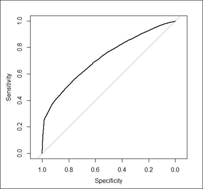
The curve derived from the model shows the area under the curve. The horizontal axis shows the false positive rate and the vertical axis shows the true positive rate. If the area under the curve is more than 70%, then the model is considered to be a good model as per industry standard:

> #Label the prediction result above the certain threshold as Yes and No

> #Change the threshold value and check which give the better result.

> train$prob <- ifelse(prob > 0.5, "Yes", "No")

>

> #print the confusion matrix between the predicted and actual response on testdata.

> t<-table(train$prob,train$IsGood.Purchase)

>

> #accuracy

> prop.table(t)

0 1

No 0.86407589 0.09229188

Yes 0.01311903 0.03051320

The threshold for classification table is 0.50 (50%) as probability. If someone wants to change the percentage of correct classified objects, then he/she can do so by putting a filter on the probability score. The following code is used to create a confusion matrix using a different probability value. From the previous classification table, it can be concluded that 90% people correctly classified.

Cubic regression

Cubic regression is another form of regression where the parameters in a linear regression model are increased up to one or two levels of polynomial calculation. Using the Cars93_1.csv dataset, let's understand the cubic regression:

> fit.6<-lm(MPG.Overall~ I(Price)^3+I(Horsepower)^3+I(RPM)^3+

+ Wheelbase+Width+Turn.circle, data=Cars93_1[-c(28,42,39,59,60,77),])

> summary(fit.6)

Call:

lm(formula = MPG.Overall ~ I(Price)^3 + I(Horsepower)^3 + I(RPM)^3 +

Wheelbase + Width + Turn.circle, data = Cars93_1[-c(28, 42,

39, 59, 60, 77), ])

Residuals:

Min 1Q Median 3Q Max

-5.279 -1.901 -0.006 1.590 8.433

Coefficients:

Estimate Std. Error t value Pr(>|t|)

(Intercept) 57.078025 12.349300 4.622 1.44e-05 ***

I(Price) -0.108436 0.065659 -1.652 0.1026

I(Horsepower) -0.024621 0.015102 -1.630 0.1070

I(RPM) 0.001122 0.000727 1.543 0.1268

Wheelbase -0.201836 0.079948 -2.525 0.0136 *

Width -0.104108 0.198396 -0.525 0.6012

Turn.circle -0.095739 0.158298 -0.605 0.5470

---

Signif. codes: 0 '***' 0.001 '**' 0.01 '*' 0.05 '.' 0.1 ' ' 1

Residual standard error: 2.609 on 80 degrees of freedom

Multiple R-squared: 0.6974, Adjusted R-squared: 0.6747

F-statistic: 30.73 on 6 and 80 DF, p-value: < 2.2e-16

> vif(fit.6)

I(Price) I(Horsepower) I(RPM) Wheelbase Width Turn.circle

4.121923 7.048971 2.418494 3.701812 7.054405 3.284228

> coefficients(fit.6)

(Intercept) I(Price) I(Horsepower) I(RPM) Wheelbase Width

57.07802478 -0.10843594 -0.02462074 0.00112168 -0.20183606 -0.10410833

Turn.circle

-0.09573848

Keeping all other parameters constant, one unit change in the independent variable would bring a multiplicative change in the dependent variable and the multiplication factor is the cube of the beta coefficients.

Penalized regression

The problem of maximum likelihood estimation comes into picture when we include large number of predictors or highly correlated predictors or both in a regression model and its failure to provide higher accuracy in regression problems gives rise to the introduction of penalized regression in data mining. The properties of maximum likelihood cannot be satisfying the regression procedure because of high variability and improper interpretation. To address the issue, most relevant subset selection came into picture. However, the subset selection procedure has some demerits. To again solve the problem, a new method can be introduced, which is popularly known as penalized maximum likelihood estimation method. There are two different variants of penalized regression that we are going to discuss here:

· Ridge regression: The ridge regression is known as L2 quadratic penalty and the equation can be represented as follows:

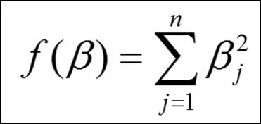
In comparison to the maximum likelihood estimates, the L1 and L2 method of estimation shrinks the beta coefficients towards zero. In order to avoid the problem of multicollinearity and higher number of predictors or both typically in a scenario when you have less number of observations, the shrinkage methods reduces the overfitted beta coefficient values.

Taking the Cars93_1.csv dataset, we can test out the model and the results from it. The lambda parameter basically strikes the balance between penalty and fit of log likelihood function. The selection of lambda value is very critical for the model; if it is a small value then the model may overfit the data and high variance would become evident, and if the lambda chosen is very large value then it may lead to biased result.

> #installing the library

> library(glmnet)

> #removing the missing values from the dataset

> Cars93_2<-na.omit(Cars93_1)

> #independent variables matrix

> x<-as.matrix(Cars93_2[,-1])

> #dependent variale matrix

> y<-as.matrix(Cars93_2[,1])

> #fitting the regression model

> mod<-glmnet(x,y,family = "gaussian",alpha = 0,lambda = 0.001)

> #summary of the model

> summary(mod)

Length Class Mode

a0 1 -none- numeric

beta 13 dgCMatrix S4

df 1 -none- numeric

dim 2 -none- numeric

lambda 1 -none- numeric

dev.ratio 1 -none- numeric

nulldev 1 -none- numeric

npasses 1 -none- numeric

jerr 1 -none- numeric

offset 1 -none- logical

call 6 -none- call

nobs 1 -none- numeric

#Making predictions

pred<-predict(mod,x,type = "link")

#estimating the error for the model.

mean((y-pred)^2)

> #Making predictions

> pred<-predict(mod,x,type = "link")

> #estimating the error for the model.

> mean((y-pred)^2)

[1] 6.663406

Given the preceding background, the regression model was able to show up with 6.66% error, which implies the model is giving 93.34% accuracy. This is not the final iteration. The model needs to be tested couple of times and various subsamples as out of the bag need to be used to conclude the final accuracy of the model.

· Least Absolute Shrinkage Operator (LASSO): The LASSO regression is known as L1 absolute value penalty (Tibshirani, 1997). The equation for LASSO regression can be expressed as follows:

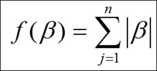
Taking the Cars93_1.csv dataset, we can test out the model and the results from it. The lambda parameter basically strikes the balance between penalty and fit of log likelihood function. The selection of the lambda value is very critical for the model; if it is a small value then the model may over fit the data and high variance would become evident, and if the lambda chosen is very large value then it may lead to biased result. Let's try to implement the model and verify the results:

> #installing the library

> library(lars)

> #removing the missing values from the dataset

> Cars93_2<-na.omit(Cars93_1)

> #independent variables matrix

> x<-as.matrix(Cars93_2[,-1])

> #dependent variale matrix

> y<-as.matrix(Cars93_2[,1])

> #fitting the LASSO regression model

> model<-lars(x,y,type = "lasso")

> #summary of the model

> summary(model)

LARS/LASSO

Call: lars(x = x, y = y, type = "lasso")

Df Rss Cp

0 1 2215.17 195.6822

1 2 1138.71 63.7148

2 3 786.48 21.8784

3 4 724.26 16.1356

4 5 699.39 15.0400

5 6 692.49 16.1821

6 7 675.16 16.0246

7 8 634.59 12.9762

8 9 623.74 13.6260

9 8 617.24 10.8164

10 9 592.76 9.7695

11 10 587.43 11.1064

12 11 551.46 8.6302

13 12 548.22 10.2275

14 13 547.85 12.1805

15 14 546.40 14.0000

The type option within the Least Angle Regression (LARS) provides opportunities to apply various variants of the lars model with "lasso", "lar", "forward.stagewise", or "stepwise". Using these we can create various models and compare the results.

From the preceding output of the model we can see the RSS and CP along with degrees of freedom, at each iterations so we need to find out a best model step where the RSS for the model is minimum:

> #select best step with a minin error

> best_model<-model$df[which.min(model$RSS)]

> best_model

14

> #Making predictions

> pred<-predict(model,x,s=best_model,type = "fit")$fit

> #estimating the error for the model.

> mean((y-pred)^2)

[1] 6.685669

The best model is available at step 14, where the RSS is minimum and hence using that best step we can make predictions. Using the predict function at that step, we can generate predictions and the error for the model chosen is 6.68%. The visualization for the fitted model can be displayed as shown next. The vertical axis shows the standardized coefficients and the horizontal axis shows the model coefficient progression for the dependent variable. The x axis shows the ratio of absolute value of beta coefficients upon the max of the absolute value of the beta coefficients. The numerator is the estimated beta coefficient current and the denominator is the beta coefficient for the OLS model. When the shrinkage parameter in LASSO takes a value of zero, the model will correspond to a OLS regression method. As the penalized parameter increases the sum of absolute values of the beta coefficients pulled to zero:

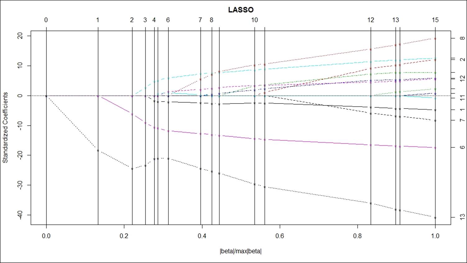
In the preceding graph, the vertical bars indicate when a variable has been pulled to zero. Vertical bar corresponding to 15 shows there are 15 predictor variables need to be reduced to zero, which corresponds to higher penalized parameter lambda value 1.0. When lambda the penalized parameter is very small, the LASSO would approach the OLS regression and as lambda increases you will see fewer variables in your model. Hence, after lambda value of 1.0, there are no variables left in the model.

L1 and L2 are known as regularized regression methods. L1 cannot zero out regression coefficients; either you will get all the coefficients or none of them. However, L2 does parameter shrinkage and variable selection automatically.

Summary

In this chapter, we discussed how to create linear regression, logistic regression, and other nonlinear regression based methods for predicting the outcome of a variable in a business scenario. Regression methods are basically very important in data mining projects, in order to create predictive models to know the future values of the unknown independent variables. We looked at various scenarios where we understood which type of model can be applied where. In the next chapter, we are going to talk about association rules or market basket analysis to understand important patterns hidden in a transactional database.