R Data Mining Blueprints (2016)
Chapter 7. Building a Retail Recommendation Engine
In this age of Internet, everything available over the Internet is not useful for everyone. Different companies and entities use different approaches to find out relevant content for their audiences. People started building algorithms to construct a relevance score, based on which recommendations could be built and suggested to the users. In my day to day life, every time I see an image on Google, 3-4 other images are recommended to me by Google, every time I look for some videos on YouTube, 10 more videos are recommended to me, every time I visit Amazon to buy some products, 5-6 products are recommended to me, and, every time I read one blog or article, a few more articles and blogs are recommended to me. This is an evidence of algorithmic forces at play to recommend certain things based on user's preferences or choices, since the user's time is precious and content available over Internet is unlimited. Hence, recommendation engine helps organizations customize their offerings based on the user's preferences so that the user does not have to spend time in exploring what is required.
In this chapter, the reader will learn the following things and their implementation using R programming language:
· What is recommendation and how does that work
· Types and methods for performing recommendation
· Implementation of product recommendation using R
What is recommendation?
Recommendation is a method or technique by which an algorithm detects what the user is looking at. Recommendation can be of products, services, food, videos, audios, images, news articles, and so on. What recommendation is can be made much clearer if we look around and note what we observe over the Internet day in and day out. For example, consider news aggregator websites and how they recommend articles to users. They look at the tags, timing of the article loaded into Internet, number of comments, likes, and shares for that article, and of course geolocation, among other details, and then model the metadata information to arrive at a score. Based on that score, they start recommending articles to new users. Same thing happens when we watch a video on YouTube. Similarly, beer recommendation system also works; the user has to select any beer at random and based on the first product chosen, the algorithm recommends other beers based on similar users' historical purchase information. Same thing happens when we buy products from online e-commerce portals.
Types of product recommendation
Broadly, there are four different types of recommendation systems that exist:
· Content-based recommendation method
· Collaborative filtering-based recommendation method
· Demographic segment-based recommendation method
· Association rule based-recommendation method
In content-based method, the terms, concepts which are also known as keywords, define the relevance. If the matching keywords from any page that the user is reading currently are found in any other content available over Internet, then start calculating the term frequencies and assign a score and based on that score whichever is closer represent that to the user. Basically, in content-based methods, the text is used to find the match between two documents so that the recommendation can be generated.
In collaborative filtering, there are two variants: user-based collaborative filtering and item-based collaborative filtering.
In user-based collaborative filtering method, the user-user similarity is computed by the algorithm and then based on their preferences the recommendation is generated. In item based collaborative filtering, item-item similarity is considered to generate recommendation.
In demographic segment based category, the age, gender, marital status, and location of the users, along with their income, job, or any other available feature, are taken into consideration to create customer segments. Once the segments are created then at a segment level the most popular product is identified and recommended to new users who belong to those respective segments.
Techniques to perform recommendation
To filter out abundant information available online and recommend useful information to the user at first hand is the prime motivation for creating recommendation engine. So how does the collaborative filtering work? Collaborative filtering algorithm generates recommendations based on a subset of users that are most similar to the active user. Each time a recommendation is requested, the algorithm needs to compute the similarity between the active user and all the other users, based on their co-rated items, so as to pick the ones with similar behaviour. Subsequently, the algorithm recommends items to the active user that are highly rated by his/her most similar users.
In order to compute the similarities between users, a variety of similarity measures have been proposed, such as Pearson correlation, cosine vector similarity, Spearman correlation, entropy-based uncertainty measure, and mean square difference. Let's look at the mathematical formula behind the calculation and implementation using R.
The objective of a collaborative filtering algorithm is to suggest new items or to predict the utility of a certain item for a particular user based on the user's previous likings and the opinions of other like-minded users.
Memory-based algorithms utilize the entire user-item database to generate a prediction. These systems employ statistical techniques to find a set of users, known as neighbours, who have a history of agreeing with the target user (that is, they either rate the same items similarly or they tend to buy similar sets of items). Once a neighbourhood of users is formed, these systems use different algorithms to combine the preferences of neighbours to produce a prediction or top-N recommendation for the active user. The techniques, also known as nearest-neighbour or user-based collaborative filtering, are very popular and widely used in practice.
Model-based collaborative filtering algorithms provide item recommendation by first developing a model of user ratings. Algorithms in this category take a probabilistic approach and envision the collaborative filtering process as computing the expected value of a user prediction, given his/her ratings on other items. The model building process is performed by different machine learning algorithms, such as Bayesian network, clustering, and rule-based approaches.
One critical step in the item-based collaborative filtering algorithm is to compute the similarity between items and then to select the most similar items. The basic idea in similarity computation between two items i and j is to first isolate the users who have rated both of these items and then to apply a similarity computation technique to determine the similarity S(i,j).
There are a number of different ways to compute the similarity between items. Here we present three such methods. These are cosine-based similarity, correlation-based similarity, and adjusted-cosine similarity:
· Cosine-based similarity: Two items are thought of as two vectors in the m dimensional user-space. The similarity between them is measured by computing the cosine of the angle between these two vectors:
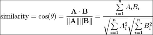
Preceding is the formula for computing cosine similarity between two vectors. Let's take a numerical example to compute the cosine similarity:
Cos (d1, d2) = 0.44
|
d1 |
d2 |
d1*d2 |
||d1|| |
||d2|| |
||d1||*||d2|| |
|
6 |
1 |
6 |
36 |
1 |
36 |
|
4 |
0 |
0 |
16 |
0 |
0 |
|
5 |
3 |
15 |
25 |
9 |
225 |
|
1 |
2 |
2 |
1 |
4 |
4 |
|
0 |
5 |
0 |
0 |
25 |
0 |
|
2 |
0 |
0 |
4 |
0 |
0 |
|
4 |
6 |
24 |
16 |
36 |
576 |
|
0 |
5 |
0 |
0 |
25 |
0 |
|
3 |
0 |
0 |
9 |
0 |
0 |
|
6 |
1 |
6 |
36 |
1 |
36 |
|
53 |
143 |
101 |
877 |
||
|
11.95826 |
10.04988 |
Table 5: Results of cosine similarity
So cosine similarity between d1 and d2 is 44%.
Cos (d1, d2) = 0.441008707
· Correlation-based similarity: Similarity between two items i and j is measured by computing the Pearson-r correlation corr. To make the correlation computation accurate, we must first isolate the co-rated cases.
· Adjusted cosine similarity: One fundamental difference between the similarity computation in user-based CF and item-based CF is that in case of user-based CF the similarity is computed along the rows of the matrix, but in case of the item-based CF the similarity is computed along the columns, that is, each pair in the co-rated set corresponds to a different user. Computing similarity using basic cosine measure in item-based case has one important drawback - the difference in rating scale between different users is not taken into account. The adjusted cosine similarity offsets this drawback by subtracting the corresponding user average from each co-rated pair. The example is given in Table 1, where the co-rated set belongs to different users, users are in different rows of the table.
Assumptions
The dataset that we are going to use for this chapter contains 100 jokes and 5000 users, which is a built-in dataset in the library recommenderlab. The dataset contains real ratings expressed by users in a scale of -10 to +10, with -10 being the worst and +10 being the best joke. We will implement various recommendation algorithms using this dataset. Using this dataset, the objective is to recommend jokes to new users based on their past preferences.
What method to apply when
Though there are four different types of recommendation methods, now which one to apply when. If the products or items are bought in a batch, then it is preferred by practitioners to apply association rules, which is also known as market basket analysis. In a retail or e-commerce domain, the items are generally purchased in a lot. Hence, when a user adds a certain product to his/her cart, other products can be recommended to him/her based on the aggregate basket component as reflected by majority of the buyers.
If the ratings or reviews are explicitly given for a set of items or products, it makes sense to apply user based collaborative filtering. If some of the ratings for few items are missing still the data can be imputed, once the missing ratings predicted, the user similarity can be computed and hence recommendation can be generated. For user-based collaborative filtering, the data would look as follows:
|
User |
Item1 |
Item2 |
Item3 |
Item4 |
Item5 |
Item6 |
|
user1 |
-7.82 |
8.79 |
-9.66 |
-8.16 |
-7.52 |
-8.5 |
|
user2 |
4.08 |
-0.29 |
6.36 |
4.37 |
-2.38 |
-9.66 |
|
user3 |
9.03 |
9.27 |
||||
|
user4 |
8.35 |
1.8 |
8.16 |
|||
|
user5 |
8.5 |
4.61 |
-4.17 |
-5.39 |
1.36 |
1.6 |
|
user6 |
-6.17 |
-3.54 |
0.44 |
-8.5 |
-7.09 |
-4.32 |
|
user7 |
8.59 |
-9.85 |
||||
|
user8 |
6.84 |
3.16 |
9.17 |
-6.21 |
-8.16 |
-1.7 |
|
user9 |
-3.79 |
-3.54 |
-9.42 |
-6.89 |
-8.74 |
-0.29 |
|
user10 |
3.01 |
5.15 |
5.15 |
3.01 |
6.41 |
5.15 |
Table 1: User-based item sample dataset
If the binary matrix is given as an input, where the levels represent whether the product is bought or not, then it is recommended to apply item-based collaborative filtering. The sample dataset is given next:
|
User |
Item1 |
Item2 |
Item3 |
Item4 |
Item5 |
Item6 |
|
user1 |
1 |
1 |
1 |
1 |
1 |
0 |
|
user2 |
1 |
1 |
0 |
0 |
1 |
|
|
user3 |
0 |
0 |
1 |
0 |
0 |
|
|
user4 |
0 |
1 |
1 |
1 |
1 |
|
|
user5 |
1 |
0 |
1 |
0 |
||
|
user6 |
0 |
0 |
1 |
0 |
||
|
user7 |
1 |
0 |
0 |
1 |
1 |
|
|
user8 |
1 |
0 |
1 |
1 |
0 |
|
|
user9 |
0 |
1 |
0 |
0 |
0 |
|
|
user10 |
1 |
0 |
1 |
1 |
1 |
1 |
Table 2: Item-based collaborative filtering sample dataset
If the product description details and the item description are given and the user search query is collected, then the similarity can be measured using content-based collaborative filtering method:
|
Title |
Search query |
|
Celestron LAND AND SKY 50TT Telescope |
good telescope |
|
(S5) 5-Port Mini Fast Ethernet Switch S5 |
mini switch |
|
(TE-S16)Tenda 10/100 Mbps 16 Ports Et... |
ethernet ports |
|
(TE-TEH2400M) 24-Port 10/100 Switch |
ethernet ports |
|
(TE-W300A) Wireless N300 PoE Access P... |
ethernet ports |
|
(TE-W311M) Tenda N150 Wireless Adapte... |
wireless adapter |
|
(TE-W311M) Tenda N150 Wireless Adapte... |
wireless adapter |
|
(TE-W311MI) Wireless N150 Pico USB Ad... |
wireless adapter |
|
101 Lighting 12 Watt Led Bulb - Pack Of 2 |
led bulb |
|
101 Lighting 7 Watt Led Bulb - Pack Of 2 |
led bulb |
Table 3: Content-based collaborative filtering sample dataset
Limitations of collaborative filtering
User-based collaborative filtering systems have been very successful in past, but their widespread use has revealed some real challenges, such as:
· Sparsity: In practice, many commercial recommender systems are used to evaluate large item sets (for example, Amazon.com recommends books and CDNow.com recommends music albums). In these systems, even active users may have purchased well under 1% of the items 1%). Accordingly, a recommender system based on nearest neighbor algorithms may be unable to make any item recommendations for a particular user. As a result, the accuracy of recommendations may be poor.
· Scalability: Nearest neighbor algorithms require computation that grows with both the number of users and the number of items. With millions of users and items, a typical web-based recommender system running existing algorithms will suffer serious scalability problems.
Practical project
The dataset contains a sample of 5000 users from the anonymous ratings data from the Jester Online Joke Recommender System collected between April 1999 and May 2003 (Gold- berg, Roeder, Gupta, and Perkins 2001). The dataset contains ratings for 100 jokes on a scale from -10 to 10. All users in the data set have rated 36 or more jokes. Let's load the recommenderlab library and the Jester5K dataset:
> library("recommenderlab")
> data(Jester5k)
> Jester5k@data@Dimnames[2]
[[1]]
[1] "j1" "j2" "j3" "j4" "j5" "j6" "j7" "j8" "j9"
[10] "j10" "j11" "j12" "j13" "j14" "j15" "j16" "j17" "j18"
[19] "j19" "j20" "j21" "j22" "j23" "j24" "j25" "j26" "j27"
[28] "j28" "j29" "j30" "j31" "j32" "j33" "j34" "j35" "j36"
[37] "j37" "j38" "j39" "j40" "j41" "j42" "j43" "j44" "j45"
[46] "j46" "j47" "j48" "j49" "j50" "j51" "j52" "j53" "j54"
[55] "j55" "j56" "j57" "j58" "j59" "j60" "j61" "j62" "j63"
[64] "j64" "j65" "j66" "j67" "j68" "j69" "j70" "j71" "j72"
[73] "j73" "j74" "j75" "j76" "j77" "j78" "j79" "j80" "j81"
[82] "j82" "j83" "j84" "j85" "j86" "j87" "j88" "j89" "j90"
[91] "j91" "j92" "j93" "j94" "j95" "j96" "j97" "j98" "j99"
[100] "j100"
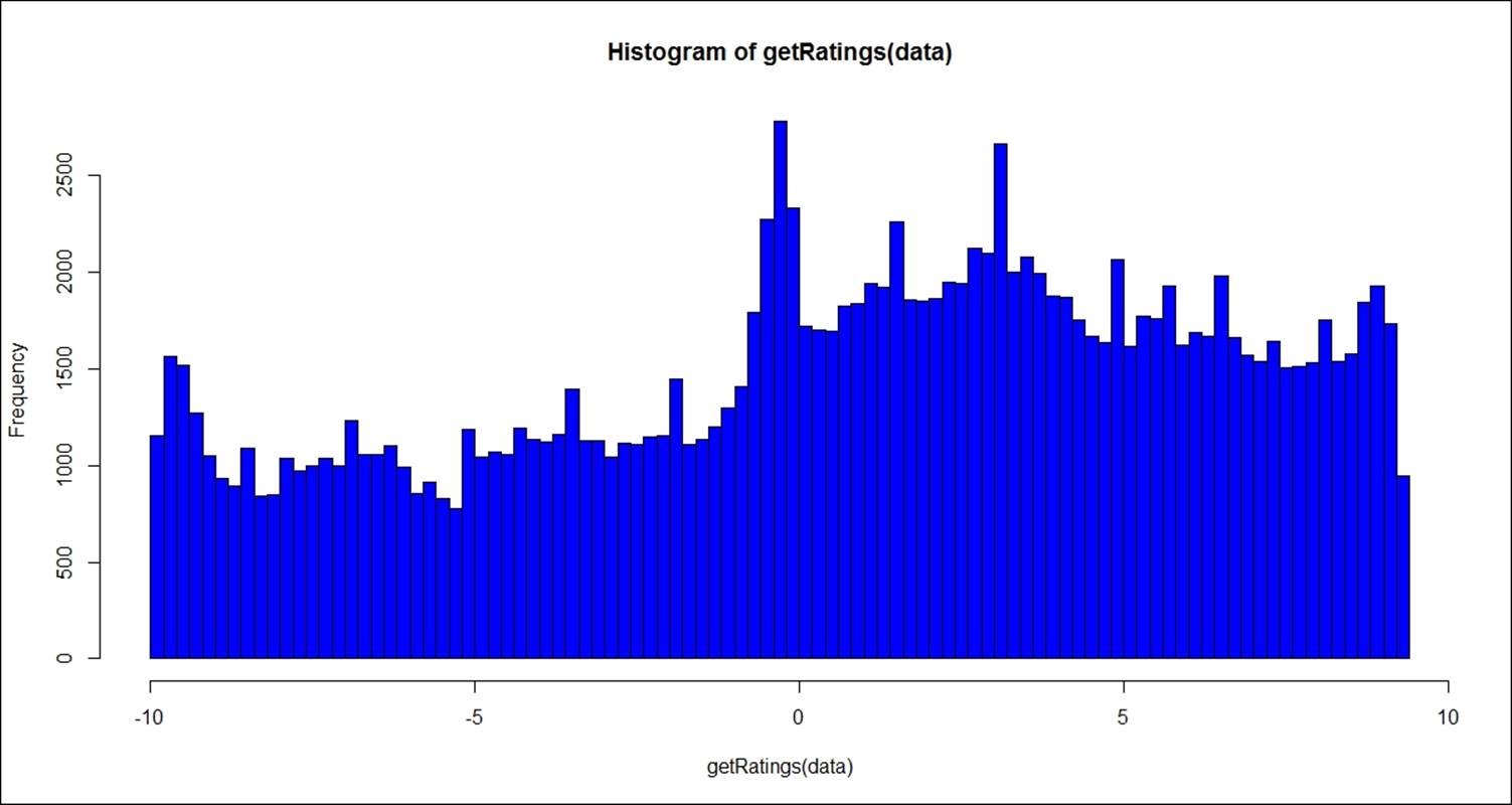
The following image shows the distribution of real ratings given by 2000 users:
> data<-sample(Jester5k,2000)
> hist(getRatings(data),breaks=100,col="blue")
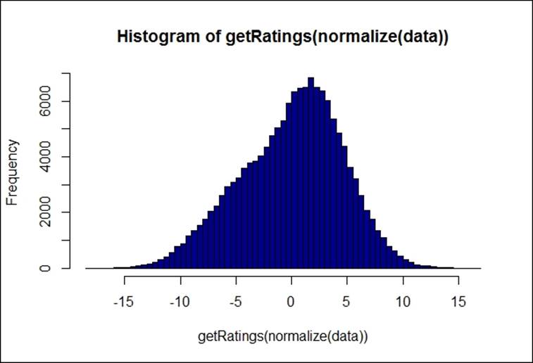
The input dataset contains the individual ratings; normalization function reduces the individual rating bias by centering the row, which is a standard z-score transformation. Subtracting each element from the mean and then dividing by standard deviation. The following graph shows normalized ratings for the preceding dataset:
> hist(getRatings(normalize(data)),breaks=100,col="blue4")
To create a recommender system:
A recommendation engine is created using the recommender() function. A new recommendation algorithm can be added by the user using the recommenderRegistry$get_entries() function:
> recommenderRegistry$get_entries(dataType = "realRatingMatrix")
$IBCF_realRatingMatrix
Recommender method: IBCF
Description: Recommender based on item-based collaborative filtering (real data).
Parameters:
k method normalize normalize_sim_matrix alpha na_as_zero minRating
1 30 Cosine center FALSE 0.5 FALSE NA
$POPULAR_realRatingMatrix
Recommender method: POPULAR
Description: Recommender based on item popularity (real data).
Parameters: None
$RANDOM_realRatingMatrix
Recommender method: RANDOM
Description: Produce random recommendations (real ratings).
Parameters: None
$SVD_realRatingMatrix
Recommender method: SVD
Description: Recommender based on SVD approximation with column-mean imputation (real data).
Parameters:
k maxiter normalize minRating
1 10 100 center NA
$SVDF_realRatingMatrix
Recommender method: SVDF
Description: Recommender based on Funk SVD with gradient descend (real data).
Parameters:
k gamma lambda min_epochs max_epochs min_improvement normalize
1 10 0.015 0.001 50 200 1e-06 center
minRating verbose
1 NA FALSE
$UBCF_realRatingMatrix
Recommender method: UBCF
Description: Recommender based on user-based collaborative filtering (real data).
Parameters:
method nn sample normalize minRating
1 cosine 25 FALSE center NA
The preceding Registry command helps in identifying the methods available in recommenderlab, parameters for the model.
There are six different methods for implementing recommender system: popular, item-based, user based, PCA, random, and SVD. Let's start the recommendation engine using popular method:
> rc <- Recommender(Jester5k, method = "POPULAR")
> rc
Recommender of type 'POPULAR' for 'realRatingMatrix'
learned using 5000 users.
> names(getModel(rc))
[1] "topN" "ratings"
[3] "minRating" "normalize"
[5] "aggregationRatings" "aggregationPopularity"
[7] "minRating" "verbose"
> getModel(rc)$topN
Recommendations as 'topNList' with n = 100 for 1 users.
The objects such as top N, verbose, aggregation popularity, and others can be printed using names of the getmodel() command.
recom <- predict(rc, Jester5k, n=5)
recom
To generate recommendation, we can use the predict function against the same dataset and validate the accuracy of the predictive model. Here we are generating top 5 recommended jokes to each of the users. The result of the prediction is as follows:
> head(as(recom,"list"))
$u2841
[1] "j89" "j72" "j76" "j88" "j83"
$u15547
[1] "j89" "j93" "j76" "j88" "j91"
$u15221
character(0)
$u15573
character(0)
$u21505
[1] "j89" "j72" "j93" "j76" "j88"
$u15994
character(0)
For the same Jester5K dataset, let's try to implement item-based collaborative filtering (IBCF):
> rc <- Recommender(Jester5k, method = "IBCF")
> rc
Recommender of type 'IBCF' for 'realRatingMatrix'
learned using 5000 users.
> recom <- predict(rc, Jester5k, n=5)
> recom
Recommendations as 'topNList' with n = 5 for 5000 users.
> head(as(recom,"list"))
$u2841
[1] "j85" "j86" "j74" "j84" "j80"
$u15547
[1] "j91" "j87" "j88" "j89" "j93"
$u15221
character(0)
$u15573
character(0)
$u21505
[1] "j78" "j80" "j73" "j77" "j92"
$u15994
character(0)
Principal component analysis (PCA) method is not applicable for real rating-based dataset because getting correlation matrix and subsequent eigen vector and eigen value calculation would not be accurate. Hence, we will not show its application. Next we are going to show how the random method works:
> rc <- Recommender(Jester5k, method = "RANDOM")
> rc
Recommender of type 'RANDOM' for 'ratingMatrix'
learned using 5000 users.
> recom <- predict(rc, Jester5k, n=5)
> recom
Recommendations as 'topNList' with n = 5 for 5000 users.
> head(as(recom,"list"))
[[1]]
[1] "j90" "j74" "j86" "j78" "j85"
[[2]]
[1] "j87" "j88" "j74" "j92" "j79"
[[3]]
character(0)
[[4]]
character(0)
[[5]]
[1] "j95" "j86" "j93" "j78" "j83"
[[6]]
character(0)
In recommendation engine, the SVD approach is used to predict the missing ratings so that recommendation can be generated. Using singular value decomposition (SVD) method, the following recommendation can be generated:
> rc <- Recommender(Jester5k, method = "SVD")
> rc
Recommender of type 'SVD' for 'realRatingMatrix'
learned using 5000 users.
> recom <- predict(rc, Jester5k, n=5)
> recom
Recommendations as 'topNList' with n = 5 for 5000 users.
> head(as(recom,"list"))
$u2841
[1] "j74" "j71" "j84" "j79" "j80"
$u15547
[1] "j89" "j93" "j76" "j81" "j88"
$u15221
character(0)
$u15573
character(0)
$u21505
[1] "j80" "j73" "j100" "j72" "j78"
$u15994
character(0)
The result from the user-based collaborative filtering is shown next:
> rc <- Recommender(Jester5k, method = "UBCF")
> rc
Recommender of type 'UBCF' for 'realRatingMatrix'
learned using 5000 users.
> recom <- predict(rc, Jester5k, n=5)
> recom
Recommendations as 'topNList' with n = 5 for 5000 users.
> head(as(recom,"list"))
$u2841
[1] "j81" "j78" "j83" "j80" "j73"
$u15547
[1] "j96" "j87" "j89" "j76" "j93"
$u15221
character(0)
$u15573
character(0)
$u21505
[1] "j100" "j81" "j83" "j92" "j96"
$u15994
character(0)
Now let's compare the results obtained from all the five different algorithms, except PCA, because PCA requires a binary dataset and does not accept real ratings matrix.
|
Popular |
IBCF |
Random method |
SVD |
UBCF |
|
> head(as(recom,"list")) |
> head(as(recom,"list")) |
> head(as(recom,"list")) |
> head(as(recom,"list")) |
> head(as(recom,"list")) |
|
$u2841 |
$u2841 |
[[1]] |
$u2841 |
$u2841 |
|
[1] "j89" "j72" "j76" "j88" "j83" |
[1] "j85" "j86" "j74" "j84" "j80" |
[1] "j90" "j74" "j86" "j78" "j85" |
[1] "j74" "j71" "j84" "j79" "j80" |
[1] "j81" "j78" "j83" "j80" "j73" |
|
$u15547 |
$u15547 |
[[2]] |
$u15547 |
$u15547 |
|
[1] "j89" "j93" "j76" "j88" "j91" |
[1] "j91" "j87" "j88" "j89" "j93" |
[1] "j87" "j88" "j74" "j92" "j79" |
[1] "j89" "j93" "j76" "j81" "j88" |
[1] "j96" "j87" "j89" "j76" "j93" |
|
$u15221 |
$u15221 |
[[3]] |
$u15221 |
$u15221 |
|
character(0) |
character(0) |
character(0) |
character(0) |
character(0) |
|
$u15573 |
$u15573 |
[[4]] |
$u15573 |
$u15573 |
|
character(0) |
character(0) |
character(0) |
character(0) |
character(0) |
|
$u21505 |
$u21505 |
[[5]] |
$u21505 |
$u21505 |
|
[1] "j89" "j72" "j93" "j76" "j88" |
[1] "j78" "j80" "j73" "j77" "j92" |
[1] "j95" "j86" "j93" "j78" "j83" |
[1] "j80" "j73" "j100" "j72" "j78" |
[1] "j100" "j81" "j83" "j92" "j96" |
|
$u15994 |
$u15994 |
[[6]] |
$u15994 |
$u15994 |
|
character(0) |
character(0) |
character(0) |
character(0) |
character(0) |
Table 4: Results comparison between different recommendation algorithms
One thing clear from the table is that for users 15573 and 15221, none of the five methods generate a recommendation. Hence, it is important to look at methods to evaluate the recommendation results. To validate the accuracy of the model let's implement accuracy measures and compare the accuracy of all the models.
For the evaluation of the model results, the dataset is divided into 90 percent for training and 10 percent for testing the algorithm. The definition of good rating is updated as 5:
> e <- evaluationScheme(Jester5k, method="split",
+ train=0.9,given=15, goodRating=5)
> e
Evaluation scheme with 15 items given
Method: 'split' with 1 run(s).
Training set proportion: 0.900
Good ratings: >=5.000000
Data set: 5000 x 100 rating matrix of class 'realRatingMatrix' with 362106 ratings.
The following script is used to build the collaborative filtering model, apply it on a new dataset for predicting the ratings and then the prediction accuracy is computed the error matrix is shown as follows:
> #User based collaborative filtering
> r1 <- Recommender(getData(e, "train"), "UBCF")
> #Item based collaborative filtering
> r2 <- Recommender(getData(e, "train"), "IBCF")
> #PCA based collaborative filtering
> #r3 <- Recommender(getData(e, "train"), "PCA")
> #POPULAR based collaborative filtering
> r4 <- Recommender(getData(e, "train"), "POPULAR")
> #RANDOM based collaborative filtering
> r5 <- Recommender(getData(e, "train"), "RANDOM")
> #SVD based collaborative filtering
> r6 <- Recommender(getData(e, "train"), "SVD")
> #Predicted Ratings
> p1 <- predict(r1, getData(e, "known"), type="ratings")
> p2 <- predict(r2, getData(e, "known"), type="ratings")
> #p3 <- predict(r3, getData(e, "known"), type="ratings")
> p4 <- predict(r4, getData(e, "known"), type="ratings")
> p5 <- predict(r5, getData(e, "known"), type="ratings")
> p6 <- predict(r6, getData(e, "known"), type="ratings")
> #calculate the error between the prediction and
> #the unknown part of the test data
> error <- rbind(
+ calcPredictionAccuracy(p1, getData(e, "unknown")),
+ calcPredictionAccuracy(p2, getData(e, "unknown")),
+ #calcPredictionAccuracy(p3, getData(e, "unknown")),
+ calcPredictionAccuracy(p4, getData(e, "unknown")),
+ calcPredictionAccuracy(p5, getData(e, "unknown")),
+ calcPredictionAccuracy(p6, getData(e, "unknown"))
+ )
> rownames(error) <- c("UBCF","IBCF","POPULAR","RANDOM","SVD")
> error
RMSE MSE MAE
UBCF 4.485571 20.12034 3.511709
IBCF 4.606355 21.21851 3.466738
POPULAR 4.509973 20.33985 3.548478
RANDOM 7.917373 62.68480 6.464369
SVD 4.653111 21.65144 3.679550
From the preceding result, UBCF has the lowest error in comparison to the other recommendation methods. Here, to evaluate the results of the predictive model, we are using k-fold cross validation method; k is assumed to be taken as 4:
> #Evaluation of a top-N recommender algorithm
> scheme <- evaluationScheme(Jester5k, method="cross", k=4,
+ given=3,goodRating=5)
> scheme
Evaluation scheme with 3 items given
Method: 'cross-validation' with 4 run(s).
Good ratings: >=5.000000
Data set: 5000 x 100 rating matrix of class 'realRatingMatrix' with 362106 ratings.
The results of the models from the evaluation scheme show the runtime versus the prediction time by different cross validation results for different models, the result is shown as follows:
> results <- evaluate(scheme, method="POPULAR", n=c(1,3,5,10,15,20))
POPULAR run fold/sample [model time/prediction time]
1 [0.14sec/2.27sec]
2 [0.16sec/2.2sec]
3 [0.14sec/2.24sec]
4 [0.14sec/2.23sec]
> results <- evaluate(scheme, method="IBCF", n=c(1,3,5,10,15,20))
IBCF run fold/sample [model time/prediction time]
1 [0.4sec/0.38sec]
2 [0.41sec/0.37sec]
3 [0.42sec/0.38sec]
4 [0.43sec/0.37sec]
> results <- evaluate(scheme, method="UBCF", n=c(1,3,5,10,15,20))
UBCF run fold/sample [model time/prediction time]
1 [0.13sec/6.31sec]
2 [0.14sec/6.47sec]
3 [0.15sec/6.21sec]
4 [0.13sec/6.18sec]
> results <- evaluate(scheme, method="RANDOM", n=c(1,3,5,10,15,20))
RANDOM run fold/sample [model time/prediction time]
1 [0sec/0.27sec]
2 [0sec/0.26sec]
3 [0sec/0.27sec]
4 [0sec/0.26sec]
> results <- evaluate(scheme, method="SVD", n=c(1,3,5,10,15,20))
SVD run fold/sample [model time/prediction time]
1 [0.36sec/0.36sec]
2 [0.35sec/0.36sec]
3 [0.33sec/0.36sec]
4 [0.36sec/0.36sec]
The confusion matrix displays the level of accuracy provided by each of the models, we can estimate the accuracy measures such as precision, recall and TPR, FPR, and so on the result is shown as follows:
> getConfusionMatrix(results)[[1]]
TP FP FN TN precision recall TPR FPR
1 0.2736 0.7264 17.2968 78.7032 0.2736000 0.01656597 0.01656597 0.008934588
3 0.8144 2.1856 16.7560 77.2440 0.2714667 0.05212659 0.05212659 0.027200530
5 1.3120 3.6880 16.2584 75.7416 0.2624000 0.08516269 0.08516269 0.046201487
10 2.6056 7.3944 14.9648 72.0352 0.2605600 0.16691259 0.16691259 0.092274243
15 3.7768 11.2232 13.7936 68.2064 0.2517867 0.24036802 0.24036802 0.139945095
20 4.8136 15.1864 12.7568 64.2432 0.2406800 0.30082509 0.30082509 0.189489883
Association rules as a method for recommendation engine for building product recommendation in a retail/e-commerce scenario, is used in Chapter 4, Regression with Automobile Data.
Summary
In this chapter, we discussed various methods of recommending products. We looked at different ways of recommending products to users, based on similarity in their purchase pattern, content, item to item comparison, and so on. As far as the accuracy is concerned, always the user-based collaborative filtering is giving better result in a real rating-based matrix as an input. Similarly, the choice of methods for a specific use case is really difficult, so it is recommended to apply all six different methods and the best one should be selected automatically and the recommendation should also get updated automatically.
All materials on the site are licensed Creative Commons Attribution-Sharealike 3.0 Unported CC BY-SA 3.0 & GNU Free Documentation License (GFDL)
If you are the copyright holder of any material contained on our site and intend to remove it, please contact our site administrator for approval.
© 2016-2026 All site design rights belong to S.Y.A.