Joe Celko's Complete Guide to NoSQL: What Every SQL Professional Needs to Know about NonRelational Databases (2014)

Chapter 13. Hierarchical and Network Database Systems

Abstract

The first true databases were based on hierarchical and network database models. These products still dominate commercial data today on mainframe commercial platforms. Failure to understand them means that you will never be able to move out of legacy systems to other platforms. This database model was defined by Charles Bachman and it influenced many other directions.

Keywords

ANSI X3H2 Database Standards Committee; Charles Bachman; CDL; CODASYL; DL/I; hierarchical database systems; IDMS; IDS (Integrated Data Store); IMS; NDL (Network Database Language); network database systems

Introduction

IMS and IDMS are the most important prerelational technologies that are still in wide use today. In fact, there is a good chance that IMS databases still hold more commercial data than SQL databases. These products still do the “heavy lifting” in banking, insurance, and large commercial applications on mainframe computers and they use COBOL. They are great for situations that do not change much and need to move around a lot of data. Because so much data still lives in them, you have to at least know the basics of hierarchical and network database systems to get to the data to put it in a NoSQL tool.

I am going to assume that most of the readers of this book have only worked with SQL. If you have heard of a hierarchical or network database system, it was probably mentioned in a database course in college and then forgotten. In some ways, this is too bad. It helps to know how the earlier tools worked, so you can see how the new tools evolve from the old ones.

13.1 Types of Databases

The classic types of database structures are network, relational, and hierarchical. The relational model is associated with Dr. E. F. Codd, and the other two models are associated with Charles Bachman, who did pioneering in the 1950s at Dow Chemical, and in the 1960’s at General Electric, where he developed the Integrated Data Store (IDS), one of the first database management systems. The network and hierarchical models are called “navigational” databases because the mental model of data access is that of a reader moving along paths to pick up the data. In fact, when Bachman received the ACM Turing Award in 1973 for his outstanding contributions to database technology, this is how he described it.

IMS was not the only navigational database, just the most popular. TOTAL from Cincom was based on a master record that had pointer chains to one or more sets of slave records. Later, IDMS and other products generalized this navigational model.

CODASYL, the committee that defined COBOL, came up with a standard for the navigational model. Finally, the ANSI X3H2 Database Standards Committee took the CODASYL model, formalized it a bit, and produced the NDL language specification. However, at that point, SQL had become the main work of the ANSI X3H2 Database Standards Committee and nobody really cared about NDL and the standard simply expired.

IMS from IBM is the most popular hierarchical database management system still in wide use today. It is stable, well defined, scalable, and very fast for what it does. The IMS software environment can be divided into five main parts:

1. Database

2. Data Language I (DL/I)

3. DL/I control blocks

4. Data communications component (IMS TM)

5. Application programs

13.2 Database History

Before the development of DBMSs, data was stored in individual files. With this system, each file was stored in a separate data set in a sequential or indexed format. To retrieve data from the file, an application had to open the file and read through it to the location of the desired data. If the data was scattered through a large number of files, data access required a lot of opening and closing of files, creating additional input/output (I/O) and processing overhead.

To reduce the number of files accessed by an application, programmers often stored the same data in many files. This practice created redundant data and the related problems of ensuring update consistency across multiple files. To ensure data consistency, special cross-file update programs had to be scheduled following the original file update.

The concept of a database system resolved many data integrity and data duplication issues encountered in a file system. A properly designed database stores the data only once in one place and makes it available to all application programs and users. At the same time, databases provide security by limiting access to data. The user’s ability to read, write, update, insert, or delete data can be restricted. Data can also be backed up and recovered more easily in a single database than in a collection of flat files.

Database structures offer multiple strategies for data retrieval. Application programs can retrieve data sequentially or (with certain access methods) go directly to the desired data, reducing I/O and speeding up data retrieval. Finally, an update performed on part of the database is immediately available to other applications. Because the data exists in only one place, data integrity is more easily ensured.

The IMS database management system as it exists today represents the evolution of the hierarchical database over many years of development and improvement. IMS is in use at a large number of business and government installations throughout the world. IMS is recognized for providing excellent performance for a wide variety of applications and for performing well with databases of moderate to very large volumes of data and transactions.

13.2.1 DL/I

Because they are implemented and accessed through use of the DL/I, IMS databases are sometimes referred to as DL/I databases. DL/I is a command-level language, not a database management system. DL/I is used in batch and online programs to access data stored in databases.

Application programs use DL/I calls to request data. DL/I then uses system access methods, such as virtual storage access method (VSAM), to handle the physical transfer of data to and from the database. IMS databases are often referred to by the access method they are designed for, such as HDAM (hierarchical direct access method), HIDAM (hierarchical indexed direct access method), PHDAM (partitioned HDAM), PHIDAM (partitioned HIDAM), HISAM (hierarchical indexed sequential access method), and SHISAM (simple HISAM). These are all IBM terms from their mainframe database products and will not be discussed here.

IMS makes provisions for nine types of access methods, and you can design a database for any one of them. On the other hand, SQL programmers are generally isolated from the access methods that their database engine uses. We will not worry about the details of the access methods that are called at this level.

13.2.2 Control Blocks

When you create an IMS database, you must define the database structure and how the data can be accessed and used by application programs. These specifications are defined within the parameters provided in two control blocks, also called DL/I control blocks:

◆ Database description (DBD)

◆ Program specification block (PSB)

In general, the DBD describes the physical structure of the database, and the PSB describes the database as it will be seen by a particular application program. The PSB tells the application which parts of the database it can access and the functions it can perform on the data. Information from the DBD and PSB is merged into a third control block, the application control block (ACB). The ACB is required for online processing but is optional for batch processing.

13.2.3 Data Communications

The IMS Transaction Manager (IMS TM) is a separate set of licensed programs that provide access to the database in an online, real-time environment. Without the TM component, you would be able to process data in the IMS database in a batch mode only.

13.2.4 Application Programs

The data in a database is of no practical use to you if it sits in the database untouched. Its value comes in its use by application programs in the performance of business or organizational functions. With IMS databases, application programs use DL/I calls embedded in the host language to access the database. IMS supports batch and online application programs. IMS supports programs written in ADA, Assembler, C, C++, COBOL, PL/I, Pascal, REXX, and WebSphere Studio Site Developer Version 5.0.

13.2.5 Hierarchical Databases

In a hierarchical database, data is grouped in records, which are subdivided into a series of segments. Consider a department database for a school in which a record consists of the segments Dept, Course, and Enroll. In a hierarchical database, the structure of the database is designed to reflect logical dependencies—certain data is dependent on the existence of certain other data. Enrollment is dependent on the existence of a course, and, in this case, a course is dependent on the existence of a department to offer that course. These are called strong and weak entities in RDBMS.

The terminology changes from the SQL world to the IMS world. IMS uses records and fields, and calls each hierarchy a database. In the SQL world, a row and column can be virtual, have defaults, and have constraints—they are smart. Records and fields are physical and depend on the application programs to give them meaning—they are dumb. In SQL, a schema or database is a collection of related tables, which might map into several different IMS hierarchies in the same data model. In other words, an IMS database is more like a table in SQL.

13.2.6 Strengths and Weaknesses

In a hierarchical database, the data relationships are defined by the storage structure. The rules for queries are highly structured. It is these fixed relationships that give IMS extremely fast access to data when compared to an SQL database when the queries have not been highly optimized.

Hierarchical and relational systems have their strengths and weaknesses. The relational structure makes it relatively easy to code ad-hoc queries. But an SQL query often makes the engine read through an entire table or series of tables to retrieve the data. This makes searches slower and more processing-intensive. In addition, because the row and column structure must be maintained throughout the database, an entry must be made under each column for every row in every table, even if the entry is only a place holder (i.e., NULL) entry.

With the hierarchical structure, data requests or segment search arguments (SSAs) may be more complex to construct. Once written, however, they can be very efficient, allowing direct retrieval of the data requested. The result is an extremely fast database system that can handle huge volumes of data transactions and large numbers of simultaneous users. Likewise, there is no need to enter placeholders where data is not being stored. If a segment occurrence isn’t needed, it isn’t created or inserted.

The trade-offs are the simplicity, portability, and flexibility of SQL versus the speed and storage savings of IMS. You tune an IMS database for one set of applications.

13.3 Simple Hierarchical Database

To illustrate how the hierarchical structure looks, we’ll design two very simple databases to store information for the courses and students in a college. One database will store information on each department in the college, and the second will contain information on each college student. In a hierarchical database, an attempt is made to group data in a one-to-many relationship.

An attempt is also made to design the database so that data that is logically dependent on other data is stored in segments that are hierarchically dependent on the data. For that reason, we have designated Dept as the key, or root, segment for our record, because the other data would not exist without the existence of a department. We list each department only once. We provide data on each course in each department. We have a segment type Course, with an occurrence of that type of segment for each course in the department. Data on the course title, description, and instructor is stored as fields within the Course segment. Finally, we have added another segment type, Enroll, which will include the student IDs of the students enrolled in each course.

Notice that we are in violation ISO-11179 naming rules. The navigational model works on one instance of a data element at a time, like a magnetic tape or punch-card file, and not on whole sets like RDBMS.

In Figure 13.1, we also created a second database called Student. This database contains information on all the students enrolled in the college. This database duplicates some of the data stored in the Enroll segment of the Department database. Later, we will construct a larger database that eliminates the duplicated data. The design we choose for our database depends on a number of factors; in this case, we will focus on which data we will need to access most frequently.

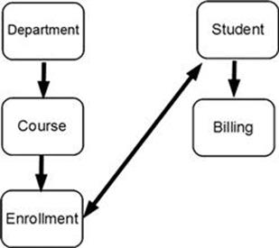
FIGURE 13.1 Sample hierarchical databases for Department and Student.

The two databases in the figure are shown as they might be structured in relational form in three tables. Notice that these tables are not always normalized when you do a direct translation to SQL. For example:

CREATE SCHEMA College;

CREATE TABLE Courses

(course_nbr CHAR(9) NOT NULL PRIMARY KEY,

course_title VARCHAR(20) NOT NULL,

course_description VARCHAR(200) NOT NULL,

dept_id CHAR(7) NOT NULL

REFERENCES Departments (dept_id)

ON UPDATE CASCADE);

CREATE TABLE Students

(student_id CHAR(9) NOT NULL PRIMARY KEY,

student_name CHAR(35) NOT NULL,

student_address CHAR(35) NOT NULL,

major CHAR(10));

CREATE TABLE Departments

(dept_id CHAR(7) NOT NULL PRIMARY KEY,

dept_name CHAR(15) NOT NULL,

chairman_name CHAR(35) NOT NULL,

budget_code CHAR(3) NOT NULL);

13.3.1 Department Database

The segments in the Department database are as follows:

◆ Dept: Information on each department. This segment includes fields for the department ID (key field), department name, chairman’s name, number of faculty, and number of students registered in departmental courses.

◆ Course: This segment includes fields for the course number (a unique identifier), course title, course description, and instructor’s name.

◆ Enroll: The students enrolled in the course. This segment includes fields for student ID (key field), student name, and grade.

13.3.2 Student Database

The segments in the Student database are as follows:

◆ Student: Student information. This segment includes fields for student ID (key field), student name, address, major, and courses completed.

◆ Billing: Billing information for courses taken. This segment includes fields for semester, tuition due, tuition paid, and scholarship funds applied.

The double-headed line between the root (Student) segment of the Student database and the Enroll segment of the Department database represents a logical relationship based on data residing in one segment and needed in the other. This is not like the referencing and referenced table structures in SQL; it has to be enforced by the application programs.

13.3.3 Design Considerations

Before implementing a hierarchical structure for your database, you should analyze the end user’s processing requirements, because they will determine how you structure the database. In particular, you must consider how the data elements are related and how they will be accessed.

For example, given the classic Parts and Suppliers database, the hierarchical structure could subordinate parts under suppliers for the accounts receivable department, or subordinate suppliers under parts for the order department. In RDBMS, there would be a relationship table that references both parts and suppliers by their primary keys and that contains information that pertains to the relationship, and not to either parts or suppliers.

13.3.4 Example Database Expanded

At this point you have learned enough about database design to expand our original example database. We decide that we can make better use of our college data by combining the Department and Student databases. Our new College database is shown in Figure 13.2.

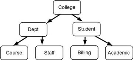
FIGURE 13.2 College database (combining Department and Student databases).

The following segments are in the expanded College database:

◆ College: The root segment. One record will exist for each college in the university. The key field is the college ID, such as ARTS, ENGR, BUSADM, and FINEARTS.

◆ Dept: Information on each department within the college. This segment includes fields for the department ID (key field), department name, chairman’s name, number of faculty, and number of students registered in departmental courses.

◆ Course: This segment includes fields for the course number (key field), course title, course description, and instructor’s name.

◆ Enroll: A list of students enrolled in the course. There are fields for student ID (key field), student name, current grade, and number of absences.

◆ Staff: A list of staff members, including professors, instructors, teaching assistants, and clerical personnel. The key field is employee number. There are fields for name, address, phone number, office number, and work schedule.

◆ Student: Student information. This segment includes fields for student ID (key field), student name, address, major, and courses being taken currently.

◆ Billing: Billing and payment information. It includes fields for billing date (key field), semester, amount billed, amount paid, scholarship funds applied, and scholarship funds available.

◆ Academic: The key field is a combination of the year and semester. Fields include grade point average (GPA) per semester, cumulative GPA, and enough fields to list courses completed and grades per semester.

13.3.5 Data Relationships

The process of data normalization helps you break data into naturally associated groupings that can be stored collectively in segments in a hierarchical database. In designing your database, break the individual data elements into groups based on the processing functions they will serve. At the same time, group data based on inherent relationships between data elements.

For example, the College database (see Figure 13.2) contains a segment called Student. Certain data is naturally associated with a student, such as student ID number, student name, address, and courses taken. Other data that wanted in the College database, such as a list of courses taught or administrative information on faculty members, would not work well in the Student segment.

Two important data relationship concepts are one-to-many and many-to-many. In the College database, there are many departments for each college, but only one college for each department. Likewise, many courses are taught by each department, but a specific course (in this case) can be offered by only one department.

The relationship between courses and students is many-to-many, as there are many students in any course and each student will take several courses. Let’s ignore the many-to-many relationship for now—this is the hardest relationship to model in a hierarchical database.

A one-to-many relationship is structured as a dependent relationship in a hierarchical database: the many are dependent on the one. Without a department, there would be no courses taught; without a college, there would be no departments.

Parent and child relationships are based solely on the relative positions of the segments in the hierarchy, and a segment can be a parent of other segments while serving as the child of a segment above it. In Figure 13.2, Enroll is a child of Course, and Course, although the parent of Enroll, is also the child of Dept. Billing and Academic are both children of Student, which is a child of College. Technically, all of the segments except College are dependents.

When you have analyzed the data elements, grouped them into segments, selected a key field for each segment, and designed a database structure, you have completed most of your database design. You may find, however, that the design you have chosen does not work well for every application program. Some programs may need to access a segment by a field other than the one you have chosen as the key. Or another application may need to associate segments that are located in two different databases or hierarchies. IMS has provided two very useful tools that you can use to resolve these data requirements: secondary indexes and logical relationships.

Secondary indexes let you create an index based on a field other than the root segment key field. That field can be used as if it were the key to access segments based on a data element other than the root key.

Logical relationships let you relate segments in separate hierarchies and, in effect, create a hierarchic structure that does not actually exist in storage. The logical structure can be processed as if it physically exists, allowing you to create logical hierarchies without creating physical ones.

13.3.6 Hierarchical Sequence

Because segments are accessed according to their sequence in the hierarchy, it is important to understand how the hierarchy is arranged. In IMS, segments are stored in a top-down, left-to-right sequence (Figure 13.3). The sequence flows from the top to the bottom of the leftmost path or leg. When the bottom of that path is reached, the sequence continues at the top of the next leg to the right.

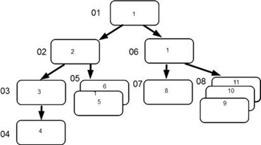
FIGURE 13.3 Sequence and data paths in a hierarchy.

Understanding the sequence of segments within a record is important to understanding movement and position within the hierarchy. Movement can be forward or backward and always follows the hierarchical sequence. Forward means from top to bottom, and backward means bottom to top. Position within the database means the current location at a specific segment. You are once more doing depth-first tree traversals, but with a slightly different terminology.

13.3.7 Hierarchical Data Paths

In Figure 13.4, the numbers inside the segments show the hierarchy as a search path would follow it. The numbers to the left of each segment show the segment types as they would be numbered by type, not occurrence. That is, there may be any number of occurrences of segment type 04, but there will be only one type of segment 04. The segment type is referred to as the segment code.

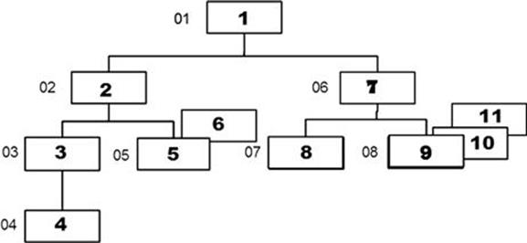
FIGURE 13.4 Hierarchical Data Paths.

To retrieve a segment, count every occurrence of every segment type in the path and proceed through the hierarchy according to the rules of navigation:

◆ Top to bottom

◆ Front to back (counting twin segments)

◆ Left to right

For example, if an application program issues a GET-UNIQUE (GU) call for segment 6 in Figure 13.4, the current position in the hierarchy is immediately following segment 06. If the program then issues a GET-NEXT (GN) call, IMS would return segment 07. There is also the GET-NEXT WITHIN PARENT (GNP) call, which explains itself.

As shown in Figure 13.4, the College database can be separated into four search paths:

◆ The first path includes segment types 01, 02, 03, and 04.

◆ The second path includes segment types 01, 02, and 05.

◆ The third path includes segment types 01, 06, and 07.

◆ The fourth path includes segment types 01, 06, and 08. The search path always starts at 01, the root segment.

13.3.8 Database Records

Whereas a database consists of one or more database records, a database record consists of one or more segments. In the College database, a record consists of the root segment College and its dependent segments. It is possible to define a database record as only a root segment. A database can contain only the record structure defined for it, and a database record can contain only the types of segments defined for it.

The term record can also be used to refer to a data set record (or block), which is not the same thing as a database record. IMS uses standard data system management methods to store its databases in data sets. The smallest entity of a data set is also referred to as arecord (or block).

Two distinctions are important. A database record may be stored in several data set blocks. A block may contain several whole records or pieces of several records. In this chapter, I try to distinguish between a database record and data set record where the meaning may be ambiguous.

13.3.9 Segment Format

A segment is the smallest structure of the database in the sense that IMS cannot retrieve data in an amount less than a segment. Segments can be broken down into smaller increments called fields, which can be addressed individually by application programs.

A database record can contain a maximum of 255 types of segments. The number of segment occurrences of any type is limited only by the amount of space you allocate for the database. Segment types can be of fixed length or variable length. You must define the size of each segment type.

It is important to distinguish the difference between segment types and segment occurrences. Course is a type of segment defined in the DBD for the College database. There can be any number of occurrences for the Course segment type. Each occurrence of theCourse segment type will be exactly as defined in the DBD. The only difference in occurrences of segment types is the data contained in them (and the length, if the segment is defined as variable length).

Segments have several different possible structures, but from a logical viewpoint, there is a prefix that has structural and control information for the IMS system, and 3 is the prefix for the actual data fields.

In the data portion, you can define the following types of fields: a sequence field and the data fields. The sequence field is often referred to as the key field. It can be used to keep occurrences of a segment type in sequence under a common parent, based on the data or value entered in this field. A key field can be defined in the root segment of a HISAM, HDAM, or HIDAM database to give an application program direct access to a specific root segment. A key field can be used in HISAM and HIDAM databases to allow database records to be retrieved sequentially. Key fields are used for logical relationships and secondary indexes.

The key field not only can contain data but also can be used in special ways that help you organize your database. With the key field, you can keep occurrences of a segment type in some kind of key sequence, which you design. For instance, in our example database you might want to store the student records in ascending sequence, based on student ID number. To do this, you define the student ID field as a unique key field. IMS will store the records in ascending numerical order. You could also store them in alphabetical order by defining the name field as a unique key field. Three factors of key fields are important to remember:

1. The data or value in the key field is called the key of the segment.

2. The key field can be defined as unique or nonunique.

3. You do not have to define a key field in every segment type

You define data fields to contain the actual data being stored in the database. (Remember that the sequence field is a data field.) Data fields, including sequence fields, can be defined to IMS for use by applications programs.

13.3.10 Segment Definitions

In IMS, segments are defined by the order in which they occur and by their relationship with other segments:

◆ Root segment: The first, or highest, segment in the record. There can be only one root segment for each record. There can be many records in a database.

◆ Dependent segment: All segments in a database record except the root segment.

◆ Parent segment: A segment that has one or more dependent segments beneath it in the hierarchy.

◆ Child segment: A segment that is a dependent of another segment above it in the hierarchy.

◆ Twin segment: A segment occurrence that exists with one or more segments of the same type under a single parent.

There are functions to edit, encrypt, or compress segments, which we will not consider here. The point is that you have a lot of control of the data at the physical level in IMS.

13.4 Summary

“Those who cannot remember the past are condemned to repeat it.” —George Santayana

There were databases before SQL, and they were all based on a navigation model. What SQL programmers do not like to admit is that not all commercial information resides in SQL databases. The majority is still in simple files or older, navigational, nonrelational databases.

Even after the new tools have taken on their own characteristics to become a separate species, the mental models of the old systems still linger. The old patterns are repeated in the new technology.

Even the early SQL products fell into this trap. For example, how many SQL programmers today use IDENTITY, or other auto-increment vendor extensions as keys on SQL tables today, unaware that they are imitating the navigational sequence field (a.k.a. the key field) from IMS?

This is not to say that a hierarchy is not a good way to organize data; it is! But you need to see the abstraction apart from any particular implementation. SQL is a declarative language, while DL/I is a collection of procedure calls inside a host language. The temptation is to continue to write SQL code in the same style as you wrote procedural code in COBOL, PL/I, or whatever host language you had.

The bad news is that you can use cursors to imitate sequential file routines. Roughly, the READ() command becomes an embedded FETCH statement, OPEN and CLOSE file commands map to OPEN CURSOR and CLOSE CURSOR statements, and every file becomes a simple table without any constraints and a “record number” of some sort. The conversion of legacy code is almost effortless with such a mapping. And it is also the worst way to program with a SQL database.

Hopefully, this book will show you a few tricks that will let you write SQL as SQL and not fake a previous language in it.

Concluding Thoughts

IMS is almost 50 years old and has moved from the early IBM System/360 technology and COBOL to LINUX and Java. Failure to understand how all that data is modeled and accessed means you cannot get to that data. My personal experience was being teased by younger programmers for not knowing the current cool application programming language. When I asked them what they were doing, they were moving IBM 3270 terminal applications onto cell phones; the back end was an IMS database that had been at their insurance company since 1970. As Alphonse Karr said in 1839: “Plus ça change, plus c’est la même chose”—“the more it changes, the more it’s the same thing.”

References

1. The www.dbazine.com website has a detailed three-part tutorial on IMS, from which this material was brutally extracted and summarized.

2. The best source for IMS materials is at http://www.redbooks.ibm.com/ where you can download manuals directly from IBM.

3. Dutta A. IMS concepts and database administration. 2010, 2012; Houston, TX. https://communities.bmc.com/docs/DOC-9908; 2010, 2012.

4. Meltz D, et al. An introduction to IMS: Your complete guide to IBM's information management system. Upper Saddle River, NJ: IBM Press (Pearson Education); 2005.