Joe Celko's Complete Guide to NoSQL: What Every SQL Professional Needs to Know about NonRelational Databases (2014)
Chapter 12. Multivalued or NFNF Databases
Abstract
Multivalued or NFNF databases violate 1NF by allowing a column to contain more than one scalar value. This model has been use for decades in commercial products but did not get a theoretical basis until much later. This chapter discusses multivalued databases.
Keywords
COBOL; Pick; nonfirst normal form (NFNF); first normal form (1NF)
Introduction
RDBMS is based on first normal form (1NF), which assumes that data is kept in scalar values in columns that are kept in rows and those records have the same structure. The multivalued model allows tables to be nested inside columns. They have a niche market that is not well known to SQL programmers. There is an algebra for this data model that is just as sound as the relational model.
In 2013, most current database programmers have never worked with anything but SQL. They did not grow up with file systems, COBOL, or any of the old network or hierarchical databases. These products are still around and run a lot of commercial applications. But we also have seen a blending of the traditional hierarchical sequential records and the set-oriented models of data. Let’s start with some history.
12.1 Nested File Structures
A flat file is a file of which the fields are all scalar values and the records have the same structure. When the relational model first came out in the 1970s, developers mistook tables for flat files. They missed the mathematics and the idea of a set. A file is read from left to right, in sequence, record by record; a table exists as a set that is the unit of work. A file stands alone while a table is part of a schema and has relationships with the rest of the schema. Frankly, a lot of developers still do not understand these concepts.
But a flat file is the easiest starting point. The next most complicated file structures have variant records. Since a file is read left to right, it can tell the computer what to expect “downstream” in the data. In COBOL, we use the OCCURS and OCCURS DEPENDING ON clauses.
I will assume most of the readers do not know COBOL. The superquick explanation is that the COBOL DATA DIVISION is like the DDL in SQL, but the data is kept in strings that have a picture (PIC) clause that shows their display format. In COBOL, display and storage formats are the same. Records are made of a hierarchy of fields, and the nesting level is shown as an integer at the start of each declaration (numbers increase with depth; the convention is to step by fives). Suppose you wanted to store your monthly sales figures for the year. You could define 12 fields, one for each month, like this:
05 MONTHLY-SALES-1 PIC S9(5)V99.
05 MONTHLY-SALES-2 PIC S9(5)V99.
05 MONTHLY-SALES-3 PIC S9(5)V99.
. . .
05 MONTHLY-SALES-12 PIC S9(5)V99.
The dash is like an SQL underscore, a period is like a semicolon in SQL, and the picture tells us that each sales amount has a sign, up to five digits for dollars and two digits for cents. You can specify the field once and declare that it repeats 12 times with the simpleOCCURS clause, like this:
05 MONTHLY-SALES OCCURS 12 TIMES PIC S9(5)V99.
The individual fields are referenced in COBOL by using subscripts, such as MONTHLY-SALES(1). The OCCURS can also be at the group level, and this is its most useful application. For example, all 25 line items on an invoice (75 fields) could be held in this group:
05 LINE-ITEMS OCCURS 25 TIMES.
10 ITEM-QUANTITY PIC 9999.
10 ITEM-DESCRIPTION PIC X(30).
10 UNIT-PRICE PIC S9(5)V99.
Notice the OCCURS is listed at the group level, so the entire group occurs 25 times.
There can be nested OCCURS. Suppose we stock 10 products and we want to keep a record of the monthly sales of each product for the past 12 months:
01 INVENTORY-RECORD.
05 INVENTORY-ITEM OCCURS 10 TIMES.
10 MONTHLY-SALES OCCURS 12 TIMES PIC 999.
In this case, INVENTORY-ITEM is a group composed only of MONTHLY-SALES, which occurs 12 times for each occurrence of an inventory item. This gives an array of 10 × 12 fields. The only information in this record is the 120 monthly sales figures—12 months for each of 10 items.
Notice that OCCURS defines an array of known size. But because COBOL is a file system language, it reads fields in records from left to right. Since there is no NULL, inserting future values that are not yet known requires some coding tricks. The language has theOCCURS DEPENDING ON option. The computer reads an integer control field and then expects to find that many occurrences of a subrecord following at runtime. Yes, this can get messy and complicated, but look at this simple patient medical treatment history record to get an idea of the possibilities:
01 PATIENT-TREATMENTS.
05 PATIENT-NAME PIC X(30).
05 PATIENT-NUMBER PIC 9(9).
05 TREATMENT-COUNT PIC 99 COMP-3.
05 TREATMENT-HISTORY OCCURS 0 TO 50 TIMES
DEPENDING ON TREATMENT-COUNT
INDEXED BY TREATMENT-POINTER.
10 TREATMENT-DATE.
15 TREATMENT-YEAR PIC 9999.
15 TREATMENT-MONTH PIC 99.
15 TREATMENT-DAY PIC 99.
10 TREATING-PHYSICIAN-NAME PIC X(30).
10 TREATMENT-CODE PIC 999.
The TREATMENT-COUNT has to be handled in the applications to correctly describe the TREATMENT-HISTORY subrecords. I will not explain COMP-3 (a data type for computations) or the INDEXED BY clause (array index), since they are not important to my point.
My point is that we had been thinking of data in arrays of nested structures before the relational model. We just had not separated data from computations and presentation layers, nor were we looking for an abstract model of computing yet.
12.2 Multivalued Systems
When mini-computers appeared, they had limited capacity compared to current hardware and software. Products that were application development systems that integrated a database with an application language were favorites among users. You could build a full application with one tool!
One of the most successful such tools was Pick. This began life as the Generalized Information Retrieval Language System (GIRLS) on an IBM System/360 in 1965 by Don Nelson and Dick Pick at TRW for use by the U.S. Army to control the inventory of Cheyenne helicopter parts.
The relational model did not exist at this time; in fact, we really did not have any data theory. The Pick file structure was made up of variable-length strings. This is not the model used in COBOL. In Pick, records are called items, fields are called attributes, and subfields are called values or subvalues (hence the present-day term multivalued database). All elements are variable length, with field and values marked off by special delimiters, so that any file, record, or field may contain any number of entries of the lower level of entity.
As a result, a Pick item (record) can be one complete entity (e.g., an entire, complete customer order) rather than an RDBMS model with a table of the set of all order headers that relates to the set of all customer order details, which relates to the inventory, etc.
The Pick system is written for a virtual machine and it included Unix-like hierarchy of directories, subdirectories, and files with records being hashed into buckets that could be scanned. There is a data dictionary that holds the system together. It also comes with a command-line language, so it is self-contained.
This made porting Pick to other platforms easy. It was quickly licensed by many distributors, so Pick became a generic name for the family of multivalued databases with an implementation of Pick/BASIC. Dick Pick founded Pick & Associates, later renamed Pick Systems, then Raining Data, and, as of 2011, TigerLogic. He licensed Pick to a large variety of manufacturers and vendors who have produced different dialects of Pick. The dialect sold by TigerLogic is now known as D3, mvBase, and mvEnterprise. Those previously sold by IBM under the U2 umbrella are known as UniData and UniVerse. Rocket Software purchased IBM’s U2 line in 2010.
Pick runs on a large assortment of microcomputers, personal computers, and mainframe computers, and is still in use as of 2013. Here is a short list of Pick family products:
◆ UniVerse (Unix based)
◆ UniData (Unix based)
◆ D3
◆ jBASE
◆ ARev
◆ Advanced Pick
◆ mvBase
◆ mvEnterprise
◆ R83
If you are old enough to remember dBase from Ashton-Tate as the first popular database product on a PC, you can compare this to how that line of development became the Xbase family of products.
Pick was first released commercially in 1973 by Microdata Corporation (and their British distributor CMC) as the Reality Operating System now supplied by Northgate Information Solutions. The Microdata implementation added a BASIC-like language called Pick/BASIC (see Data/BASIC). This became the de-facto Pick development language because it has extensions for smart terminal interface as well as the database operations.
Eventually, like all NoSQL products seem to do, they added a SQL-style language called ENGLISH (later, ACCESS, not be confused with the Microsoft database system of the same name) for retrieval and reporting. ENGLISH could not do updates at first, but later added the command REFORMAT for batch updating. ENGLISH did not have joins or other relational operators. In effect, you “prejoined” tables in Pick by using the data dictionary redefinitions for a field, which would execute a calculated lookup in another file. Data integrity has to be done in the application code.
Proprietary variations and enhancements sprouted up, but the core product has remained the same. Pick is used primarily for business data processing because its data model matches neatly to files and forms used in office work and it has a strong enthusiastic user community.
12.3 NFNF Databases
Programming languages have had a formal basis, such as FORTRAN being based on Algebra, LISP on list processing, and so forth. Data and databases did not get “academic legitimacy” until Dr. Codd invented his relational algebra. It had everything academics love—a set of math symbols, including some new ones that would drive the typesetters crazy. But it also had axioms, thanks to Armstrong.
The immediate result was a burst of papers using Dr. Codd’s relational algebra. But the next step for a modern academic is to change or drop one of the axioms to see tha you can still have a consistent formal system. In geometry, change the parallel axiom (parallel lines never meet) to something else. For example, the replacement axiom is that two parallel lines (great circles) meet at two points on the surface of a sphere. Spheres are real. and we could test the new geometry with a real-world model.
Since 1NF is the basis for RDBMS, it was the one academics played with first. And we happen to have real multivalued databases to see if it works. Most of the academic work was done by Jaeschke and Schek at IBM and Roth, Korth, and Silberschatz at the University of Texas, Austin. They added new operators to the relational algebra and calculus to handle “nested relations” while still keeping the abstract set-oriented nature of the relational model. 1NF is not convenient for handling data with complex internal structures, such as computer-aided design and manufacturing (CAD/CAM). These applications have to handle structured entities while the 1NF table only allows atomic values for attributes.
Nonfirst normal form (NFNF) databases allow a column in a table to hold nested relations, and break the rule about a column only containing scalar values drawn from a known domain. In addition to NFNF, these databases are also called 2NF, NF2, and ¬NF in the literature. Since they are not part of the ANSI/ISO standards, you will find different proprietary implementations and academic notations for their operations.
Consider a simple example of employees and their children. On a normalized schema, the employees would be in one table and their children would be in a second table that references the parent:
CREATE TABLE Personnel
(emp_name VARCHAR(20) NOT NULL PRIMARY KEY,
..);
CREATE TABLE Dependents
(dependent_name VARCHAR(20) NOT NULL PRIMARY KEY,
emp_name VARCHAR(20) NOT NULL
REFERENCES Personnel(emp_name)--- DRI actions
ON UPDATE CASCADE
ON DELETE CASCADE,
..);
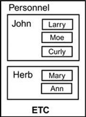
But in an NFNF schema, the dependents would be in a column with a table type, perhaps something like this:
CREATE NF TABLE Personnel
(emp_name VARCHAR(20) NOT NULL PRIMARY KEY,
dependents TABLE
(dependent_name VARCHAR(20) NOT NULL PRIMARY KEY,
emp_name VARCHAR(20) NOT NULL,
..),
..);
We can extend the basic set operators UNION, INTERSECTION, and DIFFERENCE and subsets in a natural way. Extending the relational operations is also not difficult for PROJECTION and SELECTION. The JOIN operators are a bit harder, but if you restrict your algebra to the natural or equijoin, life is easier. The important characteristic is that when these extended relational operations are used on flat tables, they behave like the original relational operations.
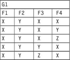
To transform this NFNF table back into a 1NF schema, you would use an UNNEST operator. The unnesting, in this case, would make Dependents into its own table and remove it from Personnel. Although UNNEST is the mathematical inverse to NEST, the operator NEST is not always the mathematical inverse of UNNEST operations. Let’s start with a simple, abstract nested table:
The UNNEST(< subtable >) operation will “flatten” a subtable up one level in the nesting:
The nest operation requires a new table name and its columns as a parameter. This is the extended SQL declaration:
NEST (G1, G2(F3, F4))
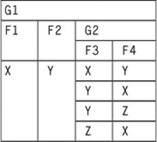
When we try to “re-nest” this step back to the original table, it fails.
There is also the question of how to order the nesting. We put the dependents inside the personnel in the first Personnel example. Children are weak entities; they have to have a parent (a strong entity) to exist. But we could have nested the parents inside the dependents. The problem is that NEST() does not commute. An operation is commutative when (A ![]() B) = (B
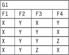
B) = (B ![]() A), if you forgot your high school algebra. Let’s start with a simple flat table:
A), if you forgot your high school algebra. Let’s start with a simple flat table:
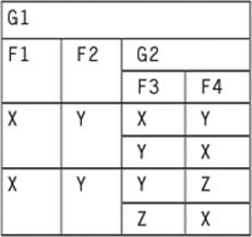
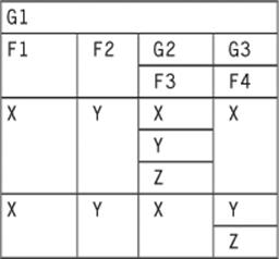
Now, we do two nestlings to create subtables G2 made up of the F3 column and G3 made up of the F4 column. First in this order:
NEST(NEST (G1, G2(F3)) , G3(F4))
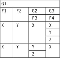
Now in the opposite order:
NEST(NEST (G1, G3(F3)) , G2(F4))
The next question is how to handle missing data. What if Herb’s daughter Mary is lactose-intolerant and has no favorite ice cream flavor in the Personnel table example? The usual NFNF model will require explicit markers instead of a generic missing value.
Another constraint required is for the operators to be objective, which is covered by the partitioned normal form (PNF). This normal form cannot have empty subtables and operations have to be reversible. A little more formally, a relation in PNF is such that its atomic attributes are a superkey of the relation and that any nonatomic component of a tuple of the relation is also in PNF.
12.4 Existing Table-Valued Extensions
Existing SQL products have added some NFNF extensions, but they are not well optimized. The syntax is usually dialect, even though there are some ANSI/ISO standards for them.
12.4.1 Microsoft SQL Server
Microsoft SQL Server 2008 added table-valued parameters and user-defined data types. The syntax lets you declare a table as a type, then use that type name to define a local variable or parameter in stored procedures. According to Microsoft, a table-valued parameter (TVP) is an efficient option for up to 1,000 or so rows. The syntax is straightforward:
CREATE TYPE Payments
AS TABLE (account_nbr CHAR(5) NOT NULL,
payment_amt DECIMAL(12,2));
This is not actually an NFNF implementation; it is more of a shorthand with limitations. You cannot use user-defined data types in a base table declaration! The T-SQL dialect uses a prefixed @ for local variables, both scalars and table variables, so to get a local, temporary table in the session, you have to write:
DECLARE @atm_money Payments;
12.4.2 Oracle Extensions
Oracle has a more powerful implementation than T-SQL, but it cannot handle optimizations without flattening the nested tables. The syntax uses Oracle’s object type in the DDL; there are other collection types in the product, but let’s create an Address_Type for a simple example. This DDL will give us an Address_Type and Address_Book table. The Address_Book is a table of Address_Type, pretty much the same syntax model at we just saw in T-SQL dialect:
CREATE TYPE Address_Type AS OBJECT
(addr_line VARCHAR2(35),
city_name VARCHAR2(25),
state_code CHAR2(2),
zip_code CHAR2(5));
CREATE TYPE Address_Book
AS TABLE OF Address_Type;
So now, to create a table, we just need to specify a column name (emp_addresses in this case) and our newly created type (Address_Book):
CREATE TABLE Personnel
(emp_name VARCHAR2(25),
emp_addresses Address_Book);
To use this table and nested table we first put the addresses objects into a base table, say Personnel. The nested table is now empty, so we have to fill it with INSERT INTO statements using the key column name. To generate a result set we can make use of the table function:
INSERT INTO Personnel(name, emp_addresses)
VALUES ('Fred Flintstone', Address_Book());
INSERT INTO TABLE
(SELECT emp_addresses
FROM Personnel
WHERE emp_name = 'Fred Flintstone')
VALUES ('123 Main', 'Bedrock', 'TX', '78787');
INSERT INTO TABLE
(SELECT emp_addresses
FROM Personnel
WHERE emp_name = 'Fred Flintstone')
VALUES ('12 Lava Ln', 'Slag Town', 'CA', '98989');
INSERT INTO TABLE
(SELECT emp_addresses
FROM Personnel
WHERE emp_name = 'Fred Flintstone')
VALUES ('77 Cave Ct', 'Pre-York', 'NY', '12121');
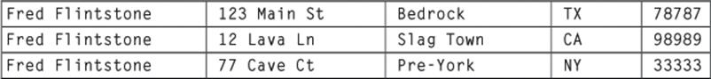
To see the results, we can flatten the nesting with a simple query. The emp_addresses table is treated something like a derived table expression, but there is an implied join condition:
SELECT T1.emp_name, T2.*
FROM Personnel AS T1,
TABLE(T1.emp_addresses) AS T2;
Concluding Thoughts
Multivalue databases is probably a better name than nonfirst normal form databases for this family of products. It is better to define something by what it is by its nature and not as the negative of something else. Most database programmers have classes on the relational model, but nobody outside a niche has any awareness of any other models, such as the multivalue one discussed here.
All materials on the site are licensed Creative Commons Attribution-Sharealike 3.0 Unported CC BY-SA 3.0 & GNU Free Documentation License (GFDL)
If you are the copyright holder of any material contained on our site and intend to remove it, please contact our site administrator for approval.
© 2016-2026 All site design rights belong to S.Y.A.