Beginning Oracle SQL: For Oracle Database 12c, Third Edition (2014)

Chapter 4. Retrieval: The Basics

In this chapter, you will start to access the seven case tables with SQL. To be more precise, you will learn how to retrieve data from your database. For data retrieval, the SQL language offers the SELECT command, introduced in Section 4.1. SQL statements that use the SELECT command are commonly referred to as queries.

An SQL statement has six main clauses. Three of them—SELECT, WHERE, and ORDER BY—are discussed in this chapter in Sections 4.2, 4.3 and 4.4, respectively. An introduction to the remaining three clauses—FROM, GROUP BY, and HAVING—is postponed until Chapter 8.

You can write queries as independent SQL statements, but queries can also occur inside other SQL statements. These are called subqueries. This chapter introduces subqueries, and then in Chapter 9, we will revisit subqueries to discuss some of their more advanced features.

Null values and their associated three-valued logic—SQL conditions have the three possible outcomes of TRUE, FALSE, or UNKNOWN—are also covered in this chapter in Section 4.9. A thorough understanding of null values and three-valued logic is critical for anyone using the SQL language. Finally, this chapter presents the truth tables of the AND, OR, and NOT operators in Section 4.10, showing how these operators handle three-valued logic.

4.1 Overview of the SELECT Command

We start this chapter with a short recap of what we already discussed in previous chapters. The six main clauses of the SELECT command are shown in Figure 4-1.

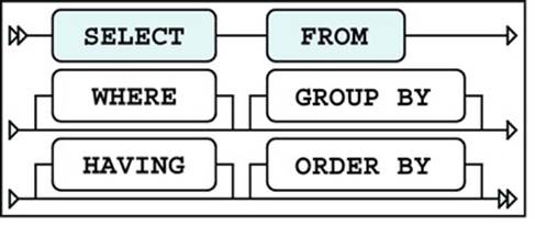
Figure 4-1. The six main clauses of the SELECT command

Figure 4-1 is identical to Figure 2-1, and it illustrates the following main syntax rules of the SELECT statement:

· There is a predefined mandatory order of these six clauses.

· The SELECT and FROM clauses are mandatory.

· WHERE, GROUP BY, HAVING, and ORDER BY are optional clauses.

Table 4-1 is identical to Table 2-1, and it shows high-level descriptions of the main SELECT command clauses.

Table 4-1. The Six Main Clauses of the SELECT Command

According to the ANSI/ISO SQL standard, these six clauses must be processed in the following order: FROM, WHERE, GROUP BY, HAVING, SELECT, ORDER BY. Note that this is not the order in which you must specify them in your queries.

As mentioned in the introduction to this chapter, SQL retrieval statements (using SELECT commands) are commonly referred to as queries. In this chapter, we will focus on queries using three SELECT command statement clauses:

· SELECT: With the SELECT clause of a SELECT command statement, you specify the columns that you want to be displayed in the query result and, optionally, which column headings you prefer to see above the result table. This clause implements the relational projectionoperator, explained in Chapter 1.

· WHERE: The WHERE clause allows you to formulate conditions that must be true in order for a row to be retrieved. In other words, this clause allows you to filter rows from the base tables; as such, it implements the relational restriction operator. You can use various operators in your WHERE clause conditions—such as BETWEEN, LIKE, IN, CASE, NOT, AND, and OR—and make them as complicated as you like.

· ORDER BY: With the ORDER BY clause, you specify the order in which you want to see the rows sorted in the result of your queries.

The FROM clause allows you to specify which tables you want to access. In this chapter, we will work with queries that access only a single table, so the FROM clause in the examples in this chapter simply specifies a single table name. The FROM clause becomes more interesting when you want to access multiple tables in a single query, as described in Chapter 8.

4.2 The SELECT Clause

Let’s start with a straightforward example of a SELECT command statement, shown in Listing 4-1.

Listing 4-1. Issuing a Simple SELECT Command

select * from departments;

DEPTNO DNAME LOCATION MGR
-------- ---------- -------- --------
10 ACCOUNTING NEW YORK 7782
20 TRAINING DALLAS 7566
30 SALES CHICAGO 7698
40 HR BOSTON 7839

The asterisk (*) symbol is used to specify that you would like all columns of the DEPARTMENTS table to be displayed in the column listing for the resultset. Listing 4-2 shows a slightly more complicated query that selects specific columns from the EMPLOYEES table and uses a WHEREclause to specify a condition for the rows retrieved.

Listing 4-2. Selecting Specific Columns

select ename, init, job, msal
from employees
where deptno = 30;

ENAME INIT JOB MSAL
-------- ----- -------- --------
ALLEN JAM SALESREP 1600
WARD TF SALESREP 1250
MARTIN P SALESREP 1250
BLAKE R MANAGER 2850
TURNER JJ SALESREP 1500
JONES R ADMIN 800

Let’s look at the syntax (the statement construction rules of a language) of this statement more closely. You have a lot of freedom in this area. For example, you can enter an entire SQL command statement in a single line, spread a SQL command statement over several lines, and use as many spaces and tabs as you like. New lines, spaces, and tabs are commonly referred to as white space. The amount of white space in your SQL statements is meaningless to the Oracle DBMS.

Tip It is a good idea to define some SQL statement layout standards and stick to them. This increases both the readability and the maintainability of your SQL statements. At this point, our SQL statements are short and simple, but in real production database environments, SQL statements are sometimes several pages long. Recall from Chapter 2 that you may also use SQL Developer formatting techniques to help you organize the layout of your SQL statements.

In the SELECT clause, white space is mandatory after the keyword SELECT. The columns (or column expressions) are separated by commas; therefore, white space is not mandatory. However, as you can see in Listing 4-2, spaces after the commas enhance readability.

White space is also mandatory after the keywords FROM and WHERE. Again, any additional white space is not mandatory, but it might enhance readability. For example, you can use spaces around the equal sign in the WHERE clause.

Column Aliases

By default, the column names of the table are displayed above your query result. If you don’t like those names—for example, because they do not adequately describe the meaning of the column in the specific context of your query—you can specify different result column headings. You include the heading you want to appear, called a column alias, in the SELECT clause of your query, as shown in the example in Listing 4-3.

Listing 4-3. Changing Column Headings

select ename, init, msal salary
from employees
where deptno = 30;

ENAME INIT SALARY
-------- ----- --------
ALLEN JAM 1600
WARD TF 1250
MARTIN P 1250
BLAKE R 2850
TURNER JJ 1500
JONES R 800

In this example, there is no comma between MSAL and SALARY. This small detail has a great effect, as the result in Listing 4-3 shows: SALARY is used instead of MSAL as a column heading (compare this with the result shown in Listing 4-2).

By the way, the ANSI/ISO SQL standard also supports the optional keyword AS between any column name and its corresponding column heading (column alias). Using this keyword enhances readability. In other words, you can also formulate the query in Listing 4-3 as follows:

select ename, init, msal AS salary
from employees
where deptno = 30;

The DISTINCT Keyword

Sometimes, your query results contain duplicate rows. You can eliminate such rows by adding the keyword DISTINCT immediately after the keyword SELECT, as demonstrated in Listing 4-4.

Listing 4-4. Using DISTINCT to Eliminate Duplicate Rows

select DISTINCT job, deptno
from employees;

JOB DEPTNO
-------- --------
ADMIN 10
ADMIN 30
DIRECTOR 10
MANAGER 10
MANAGER 20
MANAGER 30
SALESREP 30
TRAINER 20

8 rows selected.

Without the addition of the DISTINCT keyword, this query would produce 14 rows, because the EMPLOYEES table contains 14 rows. Remove the keyword DISTINCT from the first line of the query in Listing 4-4, and then execute the query again to see the difference.

Note Using DISTINCT in the SELECT clause might incur some performance overhead, because the Oracle DBMS must sort the result in order to eliminate the duplicate rows.

Column Expressions

Instead of column names, you can also specify column expressions in the SELECT clause. For example, Listing 4-5 shows how you can derive the range of the salary grades in the SALGRADES table, by selecting the difference between upper limits and lower limits.

Listing 4-5. Using a Simple Expression in a SELECT Clause

select grade, upperlimit - lowerlimit
from salgrades;

GRADE UPPERLIMIT-LOWERLIMIT
-------- ---------------------
1 500
2 199
3 599
4 999
5 6998

In the next example, shown in Listing 4-6, we concatenate the employee names with their initials into a single column, and also calculate each employee’s yearly salary by multiplying their monthly salary value by 12.

Listing 4-6. Another Example of Using Expressions in a SELECT Clause

select init||' '||ename name
, 12 * msal yearsal
from employees
where deptno = 10;

NAME YEARSAL
-------------------------------- --------
AB CLARK 29400
CC KING 60000
TJA MILLER 15600

Now take a look at the rather odd query shown in Listing 4-7.

Listing 4-7. Selecting an Expression with Literals

select 3 + 4 from departments;

3+4
--------
7
7
7
7

The query result might look strange at first; however, it makes sense when you think about it. The outcome of the expression 3+4 is calculated for each row of the DEPARTMENTS table. This is done four times, because there are four departments and we did not specify a WHERE clause. Because the expression 3+4 does not contain any variables, the result (7) is obviously the same for every department row.

The DUAL Table

It makes more sense to execute queries (that do not refer to any particular schema object (table or view), such as the one shown in Listing 4-7, against a dummy table, with only one row and one column. You could create such a table yourself, but the Oracle DBMS supplies a standard dummy table for this purpose, named DUAL, which is stored in the data dictionary. Because the Oracle DBMS knows that the DUAL table contains only one single row, you usually get better performance results by using the DUAL table rather than a dummy table that you created yourself.

Tip In 10g and above, the Oracle DBMS treats the use of DUAL like a function call that simply evaluates the expression used in the column list. This provides even better performance results than directly accessing the DUAL table.

Listing 4-8 shows two examples of DUAL table usage. Note that the contents of this DUAL table are totally irrelevant; you use only the property that the DUAL table contains a single row.

Listing 4-8. Using the DUAL Table

select 123 * 456 from dual;

123*456
--------
56088

select sysdate from dual;

SYSDATE
-----------
21-JAN-2014

The second query in Listing 4-8 shows an example of using the system date. You can refer to the system date in Oracle with the keyword SYSDATE. Actually, to be more precise, SYSDATE is a function that returns the system date. These functions are also referred to as pseudo columns. See Appendix A of this book for examples of other such pseudo columns.

Listing 4-9 shows an example of using SYSDATE to derive the age of an employee, based on the date of birth stored in the BDATE column of the EMPLOYEES table.

Listing 4-9. Using the System Date

select ename, (sysdate-bdate)/365
from employees
where empno = 7839;

ENAME (SYSDATE-BDATE)/365
-------- -------------------
KING 51.83758

Note The results of your queries using SYSDATE depend on the precise moment the command was run; therefore, when you execute the examples, the results will not be the same as those shown in Listings 4-8 and 4-9.

Null Values in Expressions

You should always consider the possibility of null values occurring in expressions. In case one or more variables in an expression evaluate to a null value, the result of the expression as a whole becomes unknown. We will discuss this area of concern in more detail later in this chapter, in Section 4.9. As a preview, please look at the result of the query in Listing 4-10.

Listing 4-10. The Effect of Null Values in Expressions

select ename, msal, comm, 12*msal + comm
from employees
where empno < 7600;

ENAME MSAL COMM 12*MSAL+COMM
-------- -------- -------- ------------
SMITH 800
ALLEN 1600 300 19500
WARD 1250 500 15500
JONES 2975

As you can see, the total yearly salary (including commission) for two out of four employees is unknown, because the commission column of those employees contains a null value.

4.3 The WHERE Clause

With the WHERE clause, you can specify a condition to filter the rows for the result. We distinguish simple and compound conditions.

Simple conditions typically contain one of the SQL comparison operators listed in Table 4-2.

Table 4-2. SQL Comparison Operators

Expressions containing comparison operators constitute statements that can evaluate to TRUE or FALSE. At least, that’s how things are in mathematics (logic), as well as in our intuition. (In Section 4.9, you will see that null values make things slightly more complicated in SQL, but for the moment, we won’t worry about them.)

Listing 4-11 shows an example of a WHERE clause with a simple condition.

Listing 4-11. A WHERE Clause with a Simple Condition

select ename, init, msal
from employees
where msal >= 3000;

ENAME INIT MSAL
-------- ----- --------
SCOTT SCJ 3000
KING CC 5000
FORD MG 3000

Listing 4-12 shows another example of a WHERE clause with a simple condition, this time using the <> (not equal to) operator.

Listing 4-12. Another Example of a WHERE Clause with a Simple Condition

select dname, location
from departments
where location <> 'CHICAGO';

DNAME LOCATION
---------- --------
ACCOUNTING NEW YORK
TRAINING DALLAS
HR BOSTON

Compound conditions consist of multiple subconditions, combined with logical operators. In Section 4.5 of this chapter, you will see how to construct compound conditions by using the logical operators AND, OR, and NOT.

4.4 The ORDER BY Clause

The result of a query is a table; that is, a set of rows. The order in which these rows appear in the result typically depends on two aspects:

· The strategy chosen by the optimizer to access the data

· The operations chosen by the optimizer to produce the desired result

This means that it is sometimes difficult to predict the order of the rows in the result. In any case, the order is not guaranteed to be the same under all circumstances.

If you insist on getting the resulting rows of your query back in a guaranteed order, you must use the ORDER BY clause in your SELECT command statements. Figure 4-2 shows the syntax of this clause.

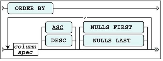
Figure 4-2. ORDER BY clause syntax diagram

As Figure 4-2 shows, you can specify multiple sort specifications, separated by commas. Each sort specification consists of a column specification (or column expression), optionally followed by the keyword DESC(descending), in case you want to sort in descending order. Without this addition, the default sorting order is ASC (ascending). ASC is underlined in Figure 4-2 to denote that it is the default.

The column specification may consist of a single column name or a column expression. To refer to columns in the ORDER BY clause, you can use any of the following:

· Regular column names

· Column aliases defined in the SELECT clause (especially useful in case of complex expressions in the SELECT clause)

· Column ordinal numbers

Column ordinal numbers in the ORDER BY clause have no relationship with the order of the columns in the database; they are dependent on only the SELECT clause of your query. Try to avoid using ordinal numbers in the ORDER BY clause. Using column aliases instead increases SQL statement readability, and ensures your ORDER BY clauses also become independent of the SELECT clauses of your queries.

Listing 4-13 shows how you can sort query results on column combinations. As you can see, the query result is sorted on department number, and then on employee name for each department.

Listing 4-13. Sorting Results with ORDER BY

select deptno, ename, init, msal
from employees
where msal < 1500
order by deptno, ename;

DEPTNO ENAME INIT MSAL
-------- -------- ---- --------
10 MILLER TJA 1300
20 ADAMS AA 1100
20 SMITH N 800
30 JONES R 800
30 MARTIN P 1250
30 WARD TF 1250

Listing 4-14 shows how you can reverse the default sorting order by adding the DESC keyword to your ORDER BY clause.

Listing 4-14. Sorting in Descending Order with ORDER BY ... DESC

select ename, 12*msal+comm as yearsal
from employees
where job = 'SALESREP'
order by yearsal desc;

ENAME YEARSAL
-------- --------
ALLEN 19500
TURNER 18000
MARTIN 16400
WARD 15500

When sorting, null values cause trouble (when don’t they, by the way?). How should columns with missing information be sorted? The rows need to go somewhere, so you need to decide. You have four options as to how to treat null values when sorting:

· Always as first values (regardless of the sorting order)

· Always as last values (regardless of the sorting order)

· As low values (lower than any existing value)

· As high values (higher than any existing value)

Figure 4-2 shows how you can explicitly indicate how to treat null values in the ORDER BY clause for each individual column expression.

Let’s try to find out Oracle’s default behavior for sorting null values. See Listing 4-15 for a first test.

Listing 4-15. Investigating the Ordering of Null Values

select evaluation
from registrations
where attendee = 7788
order by evaluation;

EVALUATION
----------
4
5

The null value in the result is tough to see; however, it is the third row. If you change the ORDER BY clause to specify a descending sort, the result becomes as shown in Listing 4-16.

Listing 4-16. Testing the Ordering of Null Values

select evaluation
from registrations
where attendee = 7788
order by evaluation DESC;

EVALUATION
----------

5
4

Listings 4-15 and 4-16 show that Oracle treats null values, by default, as high values. In other words, the default behavior is as follows:

· NULLS LAST is the default for ASC.

· NULLS FIRST is the default for DESC.

4.5 AND, OR, and NOT

You can combine simple and compound conditions into more complicated compound conditions by using the logical operators AND and OR. If you use the AND operator, you indicate that each row should evaluate to TRUE for both conditions. If you use the OR operator, only one of the conditions needs to evaluate to TRUE. Sounds easy enough, doesn’t it?

Well, the fact is that we use the words and and or in a rather sloppy way in spoken languages. The listener easily understands our precise intentions from the context, intonation, or body language. This is why there is a risk of making mistakes when translating questions from a natural language, such as English, into queries in a formal language, such as SQL.

Tip It is not uncommon to see discussions (mostly after the event) about misunderstandings in the precise wording of the original question in any natural language. Therefore, you should always try to sharpen your question in English as much as possible before trying to convert those questions into SQL statements. In cases of doubt, ask clarifying questions for this purpose.

Therefore, in SQL, the meaning of the two keywords AND and OR must be defined very precisely, without any chance for misinterpretation. You will see the formal truth tables of the AND, OR, and NOT operators in Section 4.10 of this chapter, after the discussion of null values. First, let’s experiment with these three operators and look at some examples.

The OR Operator

Consider the operator OR. We can make a distinction between the inclusive and the exclusive meaning of the word. Is it alright if both conditions evaluate to TRUE, or would it be alright if only one of the two conditions evaluates to TRUE? In natural languages, this distinction is almost always implicit. For example, suppose that you want to know when someone can meet with you, and the answer you get is “next Thursday or Friday.” In this case, you probably interpret the OR in its exclusive meaning.

What about SQL—is the OR operator inclusive or exclusive? Listing 4-17 shows the answer.

Listing 4-17. Combining Conditions with OR

select code, category, duration
from courses
where category = 'BLD'
or duration = 2;

CODE CAT DURATION
---- --- --------
JAV BLD 4
PLS BLD 1
XML BLD 2
RSD DSG 2

In this example, you can see that the OR operator in SQL is inclusive; otherwise, the third row wouldn’t show up in the result. The XML course belongs to the BLD course category (so the first condition evaluates to TRUE) and its duration is two days (so the second condition also evaluates to TRUE).

Another point of note regarding the evaluation order for an OR operator is that conditions are evaluated in order until a TRUE condition is found. All subsequent conditions are ignored. This is due to the fact that for an OR operator to be satisfied, only one condition must evaluate to TRUE. So, even if you had many OR conditions, evaluation will stop as soon as the first TRUE condition is met.

In the upcoming discussion of the NOT operator, you will see how to construct an exclusive OR.

Figure 4-3 illustrates the differences between the AND and OR operators when represented pictorially with a Venn diagram. When the OR operator is used, satisfying either condition will result in a record being returned. However, when the AND operator is used, all conditions must be satisfied before a record is returned.

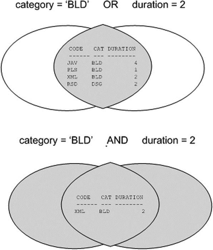
Figure 4-3. OR and AND Venn Diagram

The AND Operator and Operator Precedence Issues

There is a possible problem if your compound conditions contain a mixture of AND and OR operators. See Listing 4-18 for an experiment with a query against the DUAL table.

Listing 4-18. Combining Conditions with OR and AND

select 'is true ' as condition
from dual
where 1=1 or 1=0 and 0=1;

CONDITION
---------
is true

The compound condition in Listing 4-18 consists of three rather trivial, simple conditions, evaluating to TRUE, FALSE, and FALSE, respectively. But what is the outcome of the compound predicate as a whole, and why? Apparently, the compound predicate evaluates to TRUE; otherwise,Listing 4-18 would have returned the message “no rows selected.”

In such cases, the result depends on the operator precedence rules. You can interpret the condition of Listing 4-18 in two ways, as follows:

Listing 4-18 obviously shows an overall result of TRUE. The Oracle DBMS evaluates the expressions in the order that will require the fewest conditional checks. This decision is based on the demographics of your data and is an advanced topic not covered in this book.

With compound conditions, it is always better to use parentheses to indicate the order in which you want the operations to be performed, rather than relying on implicit language precedence rules. Listing 4-19 shows two variants of the query from Listing 4-18, using parentheses in theWHERE clause.

Listing 4-19. Using Parentheses to Force Operator Precedence

select 'is true ' as condition
from dual
where (1=1 or 1=0) and 0=1;

no rows selected

select 'is true ' as condition
from dual
where 1=1 or (1=0 and 0=1);

CONDITION
---------
is true

Caution Remember that you can use white space to beautify your SQL commands; however, never allow an attractive SQL command layout (for example, with suggestive indentations) to confuse you. Tabs, spaces, and new lines may increase statement readability, but they don’t change the meaning of your SQL statements in any way.

The NOT Operator

You can apply the NOT operator to any arbitrary condition to negate that condition. Listing 4-20 shows an example.

Listing 4-20. Using the NOT Operator to Negate Conditions

select ename, job, deptno
from employees
where NOT deptno > 10;

ENAME JOB DEPTNO
-------- -------- --------
CLARK MANAGER 10
KING DIRECTOR 10
MILLER ADMIN 10

In this simple case, you could achieve the same effect by removing the NOT operator and changing the comparison operator > into <=, as shown in Listing 4-21.

Listing 4-21. Equivalent Query Without Using the NOT Operator

select ename, job, deptno
from employees
where deptno <= 10;

ENAME JOB DEPTNO
-------- -------- --------
CLARK MANAGER 10
KING DIRECTOR 10
MILLER ADMIN 10

The NOT operator becomes more interesting and useful in cases where you have complex compound predicates with AND, OR, and parentheses. In such cases, the NOT operator gives you more control over the correctness of your commands.

In general, the NOT operator should be placed in front of the condition. Listing 4-22 shows an example of illegal syntax and a typical error message when NOT is positioned incorrectly.

Listing 4-22. Using the NOT Operator in the Wrong Place

select ename, job, deptno
from employees
where deptno NOT > 10;
where deptno NOT > 10
*
ERROR at line 3:
ORA-00920: invalid relational operator

There are some exceptions to this rule. As you will see in Section 4.6, the SQL operators BETWEEN, IN, and LIKE have their own built-in negation option.

Tip Just as you should use parentheses to avoid confusion with AND and OR operators in complex compound conditions, it is also a good idea to use parentheses to specify the precise scope of the NOT operator explicitly. See Listing 4-23 for an example.

By the way, do you remember the discussion about inclusive and exclusive OR? Listing 4-23 shows how you can construct an exclusive OR condition in an SQL statement by explicitly excluding the possibility that both OR condition evaluations evaluate to TRUE (on the fourth line). That’s why the XML course is now missing. Compare the result with Listing 4-17.

Listing 4-23. Constructing the Exclusive OR Operator

select code, category, duration
from courses
where (category = 'BLD' or duration = 2)
and not (category = 'BLD' and duration = 2);

CODE CAT DURATION
---- --- --------
JAV BLD 4
PLS BLD 1
RSD DSG 2

Just as in mathematics, you can eliminate parentheses from SQL expressions. The following two queries are logically equivalent:

select * from employees where NOT (ename = 'BLAKE' AND init = 'R')
select * from employees where ename <> 'BLAKE' OR init <> 'R'

In the second version, the NOT operator disappeared, the negation is applied to the two comparison operators, and last, but not least, the AND changes into an OR. You will look at this logical equivalence in more detail in one of the exercises at the end of this chapter.

4.6 BETWEEN, IN, and LIKE

Section 4.3 introduced the WHERE clause, and Section 4.5 explained how you can combine simple and compound conditions in the WHERE clause into more complicated compound conditions by using the logical operators AND, OR, and NOT. This section introduces three new operators you can use in simple conditions: BETWEEN, IN, and LIKE.

The BETWEEN Operator

The BETWEEN operator does not open up new possibilities; it only allows you to formulate certain conditions a bit more easily and more readably. See Listing 4-24 for an example.

Listing 4-24. Using the BETWEEN Operator

select ename, init, msal
from employees
where msal between 1300 and 1600;

ENAME INIT MSAL
-------- ----- --------
ALLEN JAM 1600
TURNER JJ 1500
MILLER TJA 1300

This example shows that the BETWEEN operator includes both border values (1300 and 1600) of the interval.

The BETWEEN operator has its own built-in negation option. Therefore, the following three SQL expressions are logically equivalent:

where msal NOT between 1000 and 2000
where NOT msal between 1000 and 2000
where msal < 1000 OR msal > 2000

The IN Operator

With the IN operator, you can compare a column or the outcome of a column expression against a list of values. Using the IN operator is also a simpler way of writing a series of OR conditions. Instead of writing empno = 7499 OR empno = 7566 OR empno = 7788, you simply use an IN-list. See Listing 4-25 for an example.

Listing 4-25. Using the IN Operator

select empno, ename, init
from employees
where empno in (7499,7566,7788);

EMPNO ENAME INIT
-------- -------- -----
7499 ALLEN JAM
7566 JONES JM
7788 SCOTT SCJ

Just like BETWEEN, the IN operator also has its own built-in negation option. The example in Listing 4-26 produces all course registrations that do not have an evaluation value of 3, 4, or 5.

Listing 4-26. Using the NOT IN Operator

select * from registrations
where evaluation NOT IN (3,4,5);

ATTENDEE COUR BEGINDATE EVALUATION
-------- ---- --------- ----------
7876 SQL 12-APR-99 2
7499 JAV 13-DEC-99 2

Check for yourself that the following four expressions are logically equivalent:

where evaluation NOT in (3,4,5)
where NOT evaluation in (3,4,5)
where NOT (evaluation=3 OR evaluation=4 OR evaluation=5)
where evaluation<>3 AND evaluation<>4 AND evaluation<>5

A rather obvious requirement for the IN operator is that all of the values you specify between the parentheses must have the same (relevant) datatype.

The LIKE Operator

You typically use the LIKE operator in the WHERE clause of your queries in combination with a search pattern. In the example shown in Listing 4-27, the query returns all courses that have something to do with SQL, using the search pattern %SQL%.

Listing 4-27. Using the LIKE Operator with the Percent Character

select * from courses
where description LIKE '%SQL%';

CODE DESCRIPTION TYP DURATION
---- ------------------------------ --- --------
SQL Introduction to SQL GEN 4
PLS Introduction to PL/SQL BLD 1

Two characters have special meaning when you use them in a string (the search pattern) after the LIKE operator. These two characters are commonly referred to as wildcards:

%: A percent sign after the LIKE operator means zero, one, or more arbitrary characters (see Listing 4-27).

_: An underscore after the LIKE operator means exactly one arbitrary character.

Note If the LIKE operator (with its two wildcard characters) provides insufficient search possibilities, you can use the REGEXP_LIKE function and regular expressions. See Chapter 5 for information about using regular expressions.

The query shown in Listing 4-28 returns all employees with an uppercase A as the second character in their name.

Listing 4-28. Using the LIKE Operator with the Percent and Underscore Characters

select empno, init, ename
from employees
where ename like '_A%';

EMPNO INIT ENAME
-------- ----- --------
7521 TF WARD
7654 P MARTIN

Just like the BETWEEN and IN operators, the LIKE operator also features a built-in negation option; in other words, you can use WHERE . . . NOT LIKE . . . .

The following queries show two special cases: one using LIKE without wildcards and one using the % character without the LIKE operator.

select * from employees where ename like 'BLAKE'
select * from employees where ename = 'BL%'

Both queries will be executed by Oracle, without any complaints or error messages. However, in the first example, we could have used the equal sign (=) instead of the LIKE operator to get the same results. In the second example, the percent sign (%) has no special meaning, since it doesn’t follow the LIKE operator, so it is very likely we would get back the “no rows selected” message.

If you really want to search for actual percent sign or underscore characters with the LIKE operator, you need to suppress the special meaning of those characters. You can do this with the ESCAPE option of the LIKE operator, as demonstrated in Listing 4-29.

Listing 4-29. Using the ESCAPE Option of the LIKE Operator

select empno, begindate, comments
from history
where comments like '%0\%%' escape '\';

EMPNO BEGINDATE COMMENTS
-------- ----------- ----------------------------------------------------
7566 01-JUN-1989 From accounting to human resources; 0% salary change
7788 15-APR-1985 Transfer to human resources; 0% salary raise

The WHERE clause in Listing 4-29 is used to filter the result set to include only those comments that include a textual reference to 0% in the COMMENTS column of the HISTORY table. The backslash (\) suppresses the special meaning of the second percent sign in the search string. Note that you can pick a character other than the backslash to use as the ESCAPE character.

4.7 CASE Expressions

You can tackle complicated procedural problems with CASE expressions. Oracle supports two CASE expression types: simpleCASE expressions and searchedCASE expressions.

Figure 4-4 illustrates the syntax of the simple CASE expression. With this type of CASE expression, you specify an input expression to be compared with the values in the WHEN ... THEN loop. The implicit comparison operator is always the equal sign. The left operand is always the input expression, and the right operand is the value from the WHEN clause.

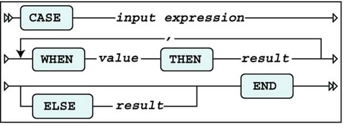
Figure 4-4. Simple CASE expression syntax diagram

Figure 4-5 shows the syntax of the searched CASE expression. The power of this type of CASE expression is that you don’t specify an input expression, but instead specify complete conditions in the WHEN clause. Therefore, you have the freedom to use any logical operator in each individual WHEN clause.

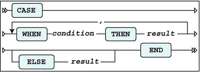
Figure 4-5. Searched CASE expressions syntax diagram

CASE expressions are evaluated as follows:

· Oracle evaluates the WHEN expressions in the order in which you specified them, and returns the THEN result of the first condition evaluating to TRUE. Note that Oracle does not evaluate the remaining WHEN clauses; therefore, the order of the WHEN expressions is important.

· If none of the WHEN expressions evaluates to TRUE, Oracle returns the ELSE expression.

· If you didn’t specify an ELSE expression, Oracle returns a null value.

Obviously, you must handle datatypes in a consistent way. The input expressions and the THEN results in the simple CASE expression (Figure 4-4) must have the same datatype, and in both CASE expression types (Figures 4-4 and 4-5), the THEN results should have the same datatype, too.

Listing 4-30 shows a straightforward example of a simple CASE expression, which doesn’t require any explanation.

Listing 4-30. Simple CASE Expression Example

select attendee, begindate
, case evaluation
when 1 then 'bad'
when 2 then 'mediocre'
when 3 then 'ok'
when 4 then 'good'
when 5 then 'excellent'
else 'not filled in'
end
from registrations
where course = 'S02';

ATTENDEE BEGINDATE CASEEVALUATIO
-------- --------- -------------
7499 12-APR-99 good
7698 12-APR-99 good
7698 13-DEC-99 not filled in
7788 04-OCT-99 not filled in
7839 04-OCT-99 ok
7876 12-APR-99 mediocre
7902 04-OCT-99 good
7902 13-DEC-99 not filled in
7934 12-APR-99 excellent

Listing 4-31 shows an example of a searched CASE expression.

Listing 4-31. Searched CASE Expression Example

select ename, job
, case when job = 'TRAINER' then ' 10%'
when job = 'MANAGER' then ' 20%'
when ename = 'SMITH' then ' 30%'
else ' 0%'
end as raise
from employees
order by raise desc, ename;

ENAME JOB RAISE
-------- -------- -----
BLAKE MANAGER 20%
CLARK MANAGER 20%
JONES MANAGER 20%
ADAMS TRAINER 10%
FORD TRAINER 10%
SCOTT TRAINER 10%
SMITH TRAINER 10%
ALLEN SALESREP 0%
JONES ADMIN 0%
KING DIRECTOR 0%
MARTIN SALESREP 0%
MILLER ADMIN 0%
TURNER SALESREP 0%
WARD SALESREP 0%

In Listing 4-31, note that SMITH gets only a 10% raise, despite the fourth line of the query. This is because he is a trainer, which causes the second line to result in a match; therefore, the remaining WHEN expressions are not considered.

Note CASE expressions may contain other CASE expressions. The only limitation is that a single CASE may have a maximum of 255 conditional expressions. Even though you can create large CASE expressions, take care to not use so many embedded conditions that your logic is hard to follow.

CASE expressions are very powerful and flexible; however, they sometimes become rather long. That’s why Oracle offers several functions that you could interpret as abbreviations (or shorthand notations) for CASE expressions, such as COALESCE and NULLIF (both of these functions are part of the ANSI/ISO SQL standard), NVL, NVL2, and DECODE. We will look at some of these functions in the next chapter.

4.8 Subqueries

Section 4.6 introduced the IN operator. This section introduces the concept of subqueries by starting with an example of the IN operator.

Suppose you want to launch a targeted e-mail campaign, because you have a brand-new course that you want to promote. The target audience for the new course is the developer community, so you want to know who attended one or more build (BLD category) courses in the past. You could execute the following query to get the desired result:

select attendee
from registrations
where course in ('JAV','PLS','XML')

This solution has at least two problems. To start with, you have looked at the COURSES table to check which courses belong to the BLD course category, apparently (evidenced by the JAV, PLS, and XML course listings in the WHERE clause). However, the original question was not referring to any specific courses; it referred to BLD courses. This lookup trick is easy in our demo database, which has a total of only ten courses, but it might be problematic, or even impossible, in real information systems. Another problem is that the solution is rather rigid. Suppose you want to repeat the e-mail promotion one year later for another new course. In that case, you may need to revise the query to reflect the current set of BLD courses.

A much better solution to this problem is to use a subquery. This way, you leave it up to the Oracle DBMS to query the COURSES table, by replacing the list of course codes between the parentheses (JAV, PLS, and XML) with a query that retrieves the desired course codes for you. Listing 4-32 shows the subquery for this example.

Listing 4-32. Using a Subquery to Retrieve All BLD Courses

select attendee
from registrations
where course in (select code
from courses
where category = 'BLD');

ATTENDEE
--------
7499
7566
7698
7788
7839
7876
7788
7782
7499
7876
7566
7499
7900

This eliminates both problems with the initial solution with the hard-coded course codes. Oracle first substitutes the subquery between the parentheses with its result—a number of course codes—and then executes the main query. (Consider “first substitutes ... and then executes ...” conceptually; the Oracle optimizer could actually decide to execute the SQL statement in a different way.)

Apparently, 13 employees attended at least one build course in the past (see Listing 4-32). Is that really true? Upon closer investigation, you can see that some employees apparently attended several build courses, or maybe some employees even attended the same build course twice. In other words, the conclusion about the number of employees (13) was too hasty. To retrieve the correct number of employees, you should use SELECTDISTINCT in the main query to eliminate duplicates.

The Joining Condition

It is always your own responsibility to formulate subqueries in such a way that you are not comparing apples with oranges. For example, the next variant of the query shown in Listing 4-33 does not result in an error message; however, the result is erroneous.

Listing 4-33. Comparing Apples with Oranges

select attendee
from registrations
where EVALUATION in (select DURATION
from courses
where category = 'BLD');

ATTENDEE
--------
7900
7788
7839
7900
7521
7902
7698
7499
7499
7876

This example compares evaluation numbers (from the main query) with course durations from the subquery. Just try to translate this query into an English sentence....

Fortunately, the Oracle DBMS does not discriminate between meaningful and meaningless questions. You have only two constraints:

· The datatypes must match, or the Oracle DBMS must be able to make them match with implicit datatype conversion.

· The subquery should not select too many column values per row.

When a Subquery Returns Too Many Values

What happens when a subquery returns too many values? Look at the query in Listing 4-34 and the resulting error message.

Listing 4-34. Error: Subquery Returns Too Many Values

select attendee
from registrations
where course in
(select course, begindate
from offerings
where location = 'CHICAGO');
(select course, begindate
*
ERROR at line 4:
ORA-00913: too many values

The subquery in Listing 4-34 returns (COURSE, BEGINDATE) value pairs, which cannot be compared with COURSE values. However, it is certainly possible to compare attribute combinations with subqueries in SQL. The query in Listing 4-34 was an attempt to find all employees who ever attended a course in Chicago.

In our data model, course offerings are uniquely identified by the combination of the course code and the begin date. Therefore, you can correct the query as shown in Listing 4-35.

Listing 4-35. Fixing the Error from Listing 4-34

select attendee
from registrations
where (course, begindate) in
(select course, begindate
from offerings
where location = 'CHICAGO');

ATTENDEE
--------
7521
7902
7900

Note Subqueries may, in turn, contain other subqueries. This principle is known as subquery nesting, and there is no practical limit to the number of subquery levels you might want to create in Oracle SQL. But be aware that at a certain level of nesting, you will probably lose the overview.

Comparison Operators in the Joining Condition

So far, we have explored subqueries with the IN operator. However, you can also establish a relationship between a main query and its subquery by using one of the comparison operators (=, <, >, <=, >=, <>), as demonstrated in Listing 4-36. In that case, there is one important difference: the subquery must return precisely one row. This additional constraint makes sense if you take into consideration how these comparison operators work: they are able to compare only a single left operand with a single right operand.

Listing 4-36. Using a Comparison Operator in the Joining Condition

select ename, init, bdate
from employees
where bdate > (select bdate
from employees
where empno = 7876);

ENAME INIT BDATE
-------- ----- ---------
JONES JM 02-APR-67
TURNER JJ 28-SEP-68
JONES R 03-DEC-69

The query in Listing 4-36 returns all employees who are younger than employee 7876. The subquery will never return more than one row, because EMPNO is the primary key of the EMPLOYEES table.

In case there is no employee with the employee number specified, you receive the “no rows selected” message. You might expect an error message like “single row subquery returns no rows” (actually, this error message once existed in Oracle, many releases ago), but apparently there is no error returned. See Listing 4-37 for an example.

Listing 4-37. When the Subquery Returns No Rows

select ename, init, bdate
from employees
where bdate > (select bdate
from employees
where empno = 99999);

no rows selected

The subquery (returning no rows, or producing an empty set) is treated like a subquery returning one row instead, containing a null value. In other words, SQL treats this situation as if there were an employee 99999 with an unknown date of birth. This may sound strange; however, this behavior is fully compliant with the ANSI/ISO SQL standard.

When a Single-Row Subquery Returns More Than One Row

In case the subquery happens to produce multiple rows, the Oracle DBMS reacts with the error message shown in Listing 4-38.

Listing 4-38. Error: Single-Row Subquery Returns More Than One Row

select ename, init, bdate
from employees
where bdate > (select bdate
from employees
where ename = 'JONES');
where bdate > (select bdate
*
ERROR at line 3:
ORA-01427: single-row subquery returns more than one row

In this example, the problem is that we have two employees with the same name (Jones). Note that you always risk this outcome, unless you make sure to use an equality comparison against a unique column of the table accessed in the subquery, as in the example in Listing 4-36.

So far, we have investigated subqueries only in the WHERE clause of the SELECT statement. Oracle SQL also supports subqueries in other SELECT statement clauses, such as the FROM clause and the SELECT clause. Chapter 9 will revisit subqueries.

4.9 Null Values

If a column (in a specific row of a table) contains no value, we say that such a column contains a null value. The term null value is actually slightly misleading, because it is an indicator of missing information. Null marker would be a better term, because a null value is not a value.

There can be many different reasons for missing information. Sometimes, an attribute is inapplicable; for example, only sales representatives are eligible for commission. An attribute value can also be unknown; for example, the person entering data did not know certain values when the data was entered. And, sometimes, you don’t know whether an attribute is applicable or inapplicable; for example, if you don’t know the job of a specific employee, you don’t know whether a commission value is applicable. The REGISTRATIONS table provides another good example. A null value in the EVALUATION column can mean several things: the course did not yet take place, the attendee had no opinion, the attendee refused to provide her opinion, the evaluation forms are not yet processed, and so on.

It would be nice if you could represent the reason why information is missing, but SQL supports only one null value, and according to Ted Codd’s Rule 3: Systematic Treatment of Missing Information (see Chapter 1) null values can have only one context-independent meaning.

Caution Don’t confuse null values with the number zero (0), a series of one or more spaces, or even an empty string. Although an empty string ('') is formally different from a null value, Oracle sometimes interprets empty strings as null values (see Chapter 6 for some examples). However, you should never rely on this (debatable) interpretation of empty strings. You should always use the reserved word NULL to refer to null values in your SQL commands. Furthermore, the Oracle documentation states that empty strings may no longer be interpreted as NULL at some point in the future.

Null Value Display

By default, null values are displayed on your computer screen as “nothing,” as shown earlier in Listings 4-15 and 4-16. You can change this behavior in SQL Developer at the session level.

You can specify how null values appear at the session level by modifying the Display NULL Value AS environment setting, available in the SQL Developer Preferences dialog box, shown in Figure 4-6. Select the Tools Preferences menu option to open this dialog box.

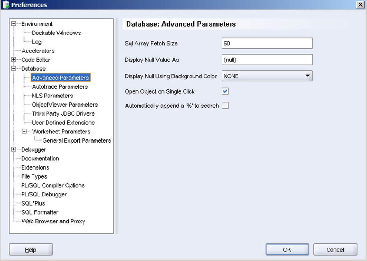
Figure 4-6. The SQL Developer Preferences dialog box

The Nature of Null Values

Null values sometimes behave counter-intuitively. Compare the results of the two queries in Listing 4-39.

Listing 4-39. Comparing Two “Complementary” Queries

select empno, ename, comm
from employees
where comm > 400;

EMPNO ENAME COMM
-------- -------- --------
7521 WARD 500
7654 MARTIN 1400

select empno, ename, comm
from employees
where comm <= 400;

EMPNO ENAME COMM
-------- -------- --------
7499 ALLEN 300
7844 TURNER 0

The first query in Listing 4-39 returns 2 employees, so you might expect to see the other 12 employees in the result of the second query, because the two WHERE clauses complement each other. However, the two query results actually are not complementary.

If Oracle evaluates a condition, there are three possible outcomes: the result can be TRUE, FALSE, or UNKNOWN. In other words, the SQL language is using three-valued logic.

Only those rows for which the condition evaluates to TRUE will appear in the result—no problem. However, the EMPLOYEES table contains several rows for which both conditions in Listing 4-39 evaluate to UNKNOWN. Therefore, these rows (ten, in this case) will not appear in either result.

Just to stress the nonintuitive nature of null values in SQL, you could say the following:

In SQL, NOT is not “not”

The explanation of this (case-sensitive) statement is that in three-valued logic, the NOT operator is not the complement operator anymore:

NOT TRUE is equivalent with FALSE
not TRUE is equivalent with FALSE OR UNKNOWN

The IS NULL Operator

Suppose you are looking for all employees except the lucky ones with a commission greater than 400. In that case, the second query in Listing 4-39 does not give you the correct answer, because you would expect to see 12 employees instead of 2. To fix this query, you need the SQL IS NULL operator, as shown in Listing 4-40.

Listing 4-40. Using the IS NULL Operator

select empno, ename, comm
from employees
where comm <= 400
or comm is null;

EMPNO ENAME COMM
-------- -------- --------
7369 SMITH
7499 ALLEN 300
7566 JONES
7698 BLAKE
7782 CLARK
7788 SCOTT
7839 KING
7844 TURNER 0
7876 ADAMS
7900 JONES
7902 FORD
7934 MILLER

Note Oracle SQL provides some functions with the specific purpose of handling null values in a flexible way (such as NVL and NVL2). These functions are covered in the next chapter.

The IS NULL operator—just like BETWEEN, IN, and LIKE—has its own built-in negation option. See Listing 4-41 for an example.

Listing 4-41. Using the IS NOT NULL Operator

select ename, job, msal, comm
from employees
where comm is not null;

ENAME JOB MSAL COMM
-------- -------- -------- --------
ALLEN SALESREP 1600 300
WARD SALESREP 1250 500
MARTIN SALESREP 1250 1400
TURNER SALESREP 1500 0

Note The IS NULL operator always evaluates to TRUE or FALSE. UNKNOWN is an impossible outcome.

Null Values and the Equality Operator

The ISNULL operator has only one operand: the preceding column name (or column expression). Actually, it is a pity that this operator is not written as IS_NULL (with an underscore instead of a space) to stress the fact that this operator has just a single operand. In contrast, the equality operator (=) has two operands: a left operand and a right operand.

Watch the rather subtle syntax difference between the following two queries:

select * from registrations where evaluation IS null
select * from registrations where evaluation = null

If you were to read both queries aloud, you might not even hear any difference. However, the seemingly innocent syntax change has definite consequences for the query results. They don’t produce error messages, because both queries are syntactically correct.

If one (or both) of the operands being compared by the equality comparison operator (=) evaluates to a null value, the result is UNKNOWN. In other words, you cannot say that a null value is equal to a null value. The following shows the conclusions:

This explains why the query in Listing 4-42 doesn’t return all 14 rows of the EMPLOYEES table.

Listing 4-42. Example of a Counterintuitive WHERE Clause

select ename, init
from employees
where comm = comm;

ENAME INIT
-------- -----
ALLEN JAM
WARD TF
MARTIN P
TURNER JJ

In mathematical logic, we call expressions always evaluating to TRUE a tautology. The example in Listing 4-42 shows that certain trivial tautologies from two-valued logic (such as COMM = COMM) don’t hold true in SQL.

Null Value Pitfalls

Null values in SQL often cause trouble. You must be aware of their existence in the database and their odds of being generated by Oracle in (intermediate) results, and you must continuously ask yourself how you want them to be treated in the processing of your SQL statements. Otherwise, the correctness of your queries will be debatable, to say the least.

You have already seen that null values in expressions generally cause those expressions to produce a null value. In the next chapter, you will learn how the various SQL functions handle null values.

It is obvious that there are many pitfalls in the area of missing information. It may be possible to circumvent at least some of these problems by properly designing your databases. In one of his books, Ted Codd, the “inventor” of the relational model, even proposed introducing two types of null values: applicable and inapplicable. This would imply the need for a four-valued logic (see The Relational Model for Database Management: Version 2 by Ted Codd (Addison-Wesley, 1990)).

Tip If you are interested in more details about null values (or other theoretical information about relational databases and pitfalls in SQL), the books written by Chris Date are the best starting point for further exploration. In particular, his Relational Database: Selected Writings series (Addison-Wesley, 1986) is brilliant. Chris Date’s ability to write in an understandable, entertaining, and fascinating way about these topics far exceeds others in the field.

Here’s a brain-twister to finish this section about null values: why does the query in Listing 4-43 produce “no rows selected”? There are registrations with evaluation values 4 and 5, for sure....

Listing 4-43. A Brain-Twister

select * from registrations
where evaluation not in (1,2,3,NULL);

no rows selected

The following WHERE clause:

where evaluation not in (1,2,3,NULL)

is logically equivalent with the following “iterated AND” condition:

where evaluation <> 1
AND evaluation <> 2
AND evaluation <> 3
AND evaluation <> NULL

If you consider a row with an EVALUATION value of 1, 2, or 3, it is obvious that out of the first three conditions, one of them returns FALSE, and the other two return TRUE. Therefore, the complete WHERE clause returns FALSE.

If the EVALUATION value is NULL, all four conditions return UNKNOWN. Therefore, the end result is also UNKNOWN. So far, there are no surprises.

If the EVALUATION value is 4 or 5 (the remaining two allowed values), the first three conditions all return TRUE, but the last condition returns UNKNOWN. So you have the following expression:

(TRUE) and (TRUE) and (TRUE) and (UNKNOWN)

This is logically equivalent with UNKNOWN, so the complete WHERE clause returns UNKNOWN. However, if you were to change the WHERE clause to read:

where evaluation not in (1,2,3)
and evaluation is not null

then the new result would return any rows with an evaluation value of 4 or 5, but no other rows.

4.10 Truth Tables

Section 4.5 of this chapter showed how to use the AND, OR, and NOT operators to build compound conditions. In that section, we didn’t worry too much about missing information and null values, but we are now in a position to examine the combination of three-valued logic and compound conditions. This is often a challenging subject, because three-valued logic is not always intuitive. The most reliable way to investigate compound conditions is to use truth tables.

Table 4-3 shows the truth table of the NOT operator. In truth tables, UNK is commonly used as an abbreviation for UNKNOWN.

Table 4-3. Truth Table of the NOT Operator

In Table 4-3, Op1 stands for the operand. Since the NOT operator works on a single operand, the truth table needs three rows to describe all possibilities. Note that the negation of UNK is UNK.

Table 4-4 shows the truth table of the AND and OR operators; Op1 and Op2 are the two operands, and the truth table shows all nine possible combinations.

Table 4-4. Truth Table of the AND and OR Operators

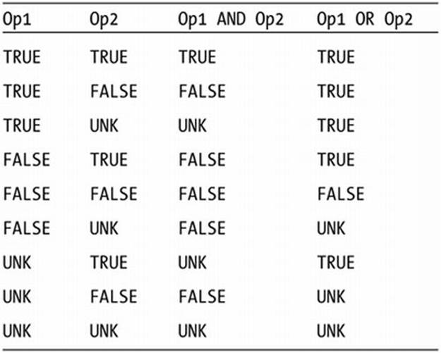
Note that the AND and OR operators are symmetric; that is, you can swap Op1 and Op2 without changing the operator outcome.

If you are facing complicated compound conditions, truth tables can be very useful to rewrite those conditions into simpler, logically equivalent, expressions.

4.11 Exercises

These exercises assume you have access to a database schema with the seven case tables (see Appendix A of this book). You can download the scripts to create this schema from this book’s catalog page on the Apress website. The exact URL ishttp://www.apress.com/9781430271970. Look in the “Source Code/Downloads” section of the catalog page for a link to the download.

When you’re done with the exercises, check your answers against ours. We give our answers in Appendix B.

1. Provide the code and description of all courses with an exact duration of four days.

2. List all employees, sorted by job, and per job by age (from young to old).

3. Which courses have been held in Chicago and/or in Seattle?

4. Which employees attended both the Java course and the XML course? (Provide their employee numbers.)

5. List the names and initials of all employees, except for R. Jones.

6. Find the number, job, and date of birth of all trainers and sales representatives born before 1960.

7. List the numbers of all employees who do not work for the training department.

8. List the numbers of all employees who did not attend the Java course.

9. Which employees have subordinates? Which employees don’t have subordinates?

10.Produce an overview of all general course offerings (course category GEN) in 1999.

11.Provide the name and initials of all employees who have ever attended a course taught by N. Smith. Hint: Use subqueries, and work “inside out” toward the result; that is, retrieve the employee number of N. Smith, then search for the codes of all courses he ever taught, and so on.

12.How could you redesign the EMPLOYEES table to avoid the problem that the COMM column contains null values meaning not applicable?

13.In Section 4.9, you saw the following statement: In SQL, NOT is not “not.” What is this statement trying to say?

14.At the end of Section 4.5, you saw the following statement.

The following two queries are logically equivalent:

select * from employees where NOT (ename = 'BLAKE' AND init = 'R')
select * from employees where ename <> 'BLAKE' OR init <> 'R'

Prove this, using a truth table. Hint: Use P as an abbreviation for ename = 'BLAKE', and use Q as an abbreviation for init = 'R'.