Expert Oracle SQL: Optimization, Deployment, and Statistics (2014)
PART 1. Basic Concepts
CHAPTER 3. Basic Execution Plan Concepts
Now that you know what the CBO is and what it does, you need to begin understanding how to interpret its output: the execution plan. You will often hear an execution plan referred to as an explain plan because the SQL explain plan statement is a key part of one the most important ways to view an execution plan. This chapter looks in detail at the explain plan statement and other ways of viewing execution plans.
But there is little point in displaying execution plans if you can’t understand what is displayed, and I will explain the process of interpreting execution plans in this chapter. Unfortunately, some execution plans are extremely complex, so I will look at the more advanced topics of execution plan interpretation in Chapter 8 after covering a little more groundwork.
Returning to this chapter, let us get started with a look at the various views that hold information about execution plans.
Displaying Execution Plans
Execution plans are to be found in several places in an Oracle database, but the following three places are the most important for the purposes of this book.
· SYS.PLAN_TABLE$: This system-owned global temporary table is usually referred to via the public synonym PLAN_TABLE and contains the results of EXPLAIN PLAN statements.
· V$SQL_PLAN: This view shows the execution plans of statements that are currently running or have recently completed running. The data that the view displays is held in the cursor cachethat is part of the shared pool.
· DBA_HIST_SQL_PLAN: This view shows a useful subset of execution plans that were executed in the past. The data that the view displays is held in the AWR and is collected from the shared pool by the MMON background process.
Although it is possible to look at the table and the two views directly, it is inconvenient to do so. This is particularly true for the OTHER_XML column that, as you might guess, contains unformatted XML. It is far easier to use functions from the DBMS_XPLAN package that present the execution plans in a more human readable format. In the following sections I will discuss how to interpret the default output of three of the package’s functions; I will look at non-default output formats in Chapters 4 and 8.
Displaying the Results of EXPLAIN PLAN
The raison d’être for the EXPLAIN PLAN SQL statement is to generate an execution plan for a statement without actually executing the statement. The EXPLAIN PLAN statement only writes a representation of the execution plan to a table. It doesn’t display anything itself. For that, you have to use the DBMS_XPLAN.DISPLAY function. This function takes several arguments, all of which are optional; I will use the defaults for now. The intention is to pass the results of the function to the TABLE operator. Listing 3-1 shows an example that performs an EXPLAIN PLAN for a query using tables from the SCOTT example schema and then displays the results using DBMS_XPLAN.DISPLAY.
Listing 3-1. Join of EMP and DEPT tables
SET LINES 200 PAGESIZE 0 FEEDBACK OFF
EXPLAIN PLAN
FOR
SELECT e.*
,d.dname
,d.loc
,(SELECT COUNT (*)
FROM scott.emp i
WHERE i.deptno = e.deptno)
dept_count
FROM scott.emp e, scott.dept d
WHERE e.deptno = d.deptno;
SELECT * FROM TABLE (DBMS_XPLAN.display);
Plan hash value: 4153889731
---------------------------------------------------------------------------
| Id | Operation | Name | Rows | Bytes | Cost (%CPU)| Time |
---------------------------------------------------------------------------
| 0 | SELECT STATEMENT | | 14 | 1638 | 7 (15)| 00:00:01 |
| 1 | SORT AGGREGATE | | 1 | 13 | | |
|* 2 | TABLE ACCESS FULL| EMP | 1 | 13 | 3 (0)| 00:00:01 |
|* 3 | HASH JOIN | | 14 | 1638 | 7 (15)| 00:00:01 |
| 4 | TABLE ACCESS FULL| DEPT | 4 | 120 | 3 (0)| 00:00:01 |
| 5 | TABLE ACCESS FULL| EMP | 14 | 1218 | 3 (0)| 00:00:01 |
---------------------------------------------------------------------------
Predicate Information (identified by operation id):
---------------------------------------------------
2 - filter("I"."DEPTNO"=:B1)
3 - access("E"."DEPTNO"="D"."DEPTNO")
Note
-----
- dynamic sampling used for this statement (level=2)
The statement being explained shows the details of each employee together with details of the department, including the estimated count of employees in the department obtained from a correlated subquery in the select list. The output of DBMS_XPLAN.DISPLAY begins with a plan hash value. If two plans have the same hash value they will be the same plan. In fact, the same execution plan will have the same hash value on different databases, provided that the operations, object names, and predicates are all identical.
After the plan hash value you can see the operation table, which provides details of how the runtime engine is expected to set about executing the SQL statement.
· The first column is the ID. This is just a number to uniquely identify the operations in the statement for use by other parts of the plan. You will notice that there is an asterisk in front of operations with IDs 2 and 3. This is because they are referred to later in the output. For the sake of brevity I will say “operation 2” rather than “The operation with ID 2” from now on.
· The second column is the operation. There are some 200 operation codes, very few of which are officially documented, and the list grows longer with each release. Fortunately, the vast majority of operations in the vast majority of execution plans come from a small subset of a couple of dozen that will become familiar to you as you read this book, if they aren’t already.
· The third column in the operation table is called name. This rather non-descript column heading refers to the name of the database object that is being operated on, so to speak. This column isn’t applicable to all operations and so is often blank, but in the case of a TABLE ACCESS FULL operation it is the name of the table being scanned.
· The next column is rows. This column provides the estimated number of rows that the operation is finally going to produce, a figure often referred to as a cardinality estimate. So, for example, you can see that operation 2 uses the TABLE ACCESS FULL operation onEMP and will read the same number of rows as ID 5 that performs the same operation on the same object. However, ID 5 returns all 14 rows in the table while operation 2 is expected to return one row. You will see the reason for this discrepancy shortly. Sometimes individual operations are executed more than once in the course of a single execution of a SQL statement. It is important to understand that the estimated row count usually applies to a single invocation of that operation and not the total number of rows returned by all invocations. In this case, operations 1 and 2 correspond to the subquery in the select list and are expected to return an average of about one row each time they are invoked.
· The bytes column shows an estimate of the number of bytes returned by one invocation of the operation. In other words, it is the average number of rows multiplied by the average size of a row.
· The cost column and the time column both display the estimated elapsed time for the statement. The cost column expresses this elapsed time in terms of single-block read units, and the time column expresses it in more familiar terms. When larger values are displayed it is possible to work out from these figures how long the CBO believes a single-block read will take by dividing time by cost. Here the small numbers and rounding make that difficult. You can also see that the cost column shows an estimate of the percentage of time that the operation will spend on the CPU as opposed to reading data from disk.
ROUNDING ISSUES
The numbers displayed in this table are always integers or seconds, but in fact the CBO keeps estimates in fractions. The rows column is rounded up and is almost always at least one, even if the CBO believes that the chances of a row being returned by the operation are slim to none. The cost column is rounded up to the nearest whole number, and the time column is rounded up the nearest second. So as a rule of thumb, always read a cardinality estimate of 1 as meaning “0 or 1.”
There are other columns that you might see in the operation table. These include columns relating to temporary space utilization, partition elimination, parallel query operations, and so on. However, these are not shown here because they aren’t relevant to this query.
Following the operation table you can see a section on predicates. In this query there are two predicates.
· The first one listed relates to operation 2. This is a filter predicate, which means that the predicate is applied to rows after the operation has generated them but before they are output. In this case the rows are rejected from the TABLE ACCESS FULL operation unless the column DEPTNO matches a particular value. But what value? The value :B1 looks for all the world to be a bind variable, but there aren’t any bind variables in this query! In fact, if you try and match up the operation to the original SQL text you will see that the table with an alias of I is, in fact, from a correlated subquery and the “variable” is actually just the corresponding DEPTNO appropriate to that invocation of the correlated subquery; in other words, it is the value from the table with alias E.
· The second predicate listed is an access predicate. This means that it is actually used as part of the execution of the operation, not just applied at the end like a filter predicate. In this case the HASH JOIN of operation 3 uses the predicate to actually perform the join.
The final section listed is a human readable note. This lists information that might be useful and that doesn’t have a place elsewhere in the plan. In this case, there are no statistics for the tables in the data dictionary, and so dynamic sampling was used to generate some statistics on the fly.
EXPLAIN PLAN May Be Misleading
When you use EXPLAIN PLAN you might expect that when you actually run the statement the execution plan that the runtime engine uses will match that from the immediately preceding EXPLAIN PLAN call. This is a dangerous assumption! Let me provide one scenario where this may not be the case.
· You run a statement. The CBO generates a plan based on the statistics available at the time and saves it in the cursor cache for the runtime engine to use.
· You gather (or set) statistics without specifying NO_INVALIDATE=FALSE. As a consequence, the execution plan saved in the cursor cache is not invalidated.
· You issue EXPLAIN PLAN. The CBO generates a plan based on the new statistics.
· You run your statement. The CBO doesn’t generate a new plan, as there is a valid execution plan already in the cursor cache. The runtime engine uses the saved plan based on the older statistics.
This isn’t the only scenario where EXPLAIN PLAN may be misleading. I will look at a feature known as bind variable peeking in Chapter 8. It is also worth bearing in mind that, for some reason, possibly security related, the SQL*Plus AUTOTRACE feature uses EXPLAIN PLAN rather than attempting to retrieve the actual execution plan from the cursor cache. So AUTOTRACE can be misleading as well.
Let us move away from EXPLAIN PLAN now and look at other ways to display execution plans.
Displaying Output from the Cursor Cache
Since the call to EXPLAIN PLAN is potentially misleading, it is very fortunate indeed that actual execution plans from the cursor cache can usually be retrieved either while a statement is running or shortly thereafter. The code in Listing 3-2 actually runs a SQL statement and then retrieves the plan from the cursor cache. By default, DBMS_XPLAN.DISPLAY_CURSOR retrieves the plan from the most recently executed SQL statement of the calling session.
Listing 3-2. Looking at execution plans in the cursor cache
SELECT 'Count of sales: ' || COUNT (*) cnt
FROM sh.sales s JOIN sh.customers c USING (cust_id)
WHERE cust_last_name = 'Ruddy';
SELECT * FROM TABLE (DBMS_XPLAN.display_cursor);
Count of sales: 1385
SELECT * FROM TABLE (DBMS_XPLAN.display_cursor);
SQL_ID d4sba28503nxy, child number 0
-------------------------------------
SELECT 'Count of sales: ' || COUNT (*) cnt FROM sh.sales s JOIN
sh.customers c USING (cust_id) WHERE cust_last_name = 'Ruddy'
Plan hash value: 1818178872
-------------------------------------------------------------------------------------
| Id | Operation | Name |X| Cost (%CPU)| Time | Pstart| Pstop |
-------------------------------------------------------------------------------------
| 0 | SELECT STATEMENT | |X| 832 (100)| | | |
| 1 | SORT AGGREGATE | |X| | | | |
|* 2 | HASH JOIN | |X| 832 (1)| 00:00:08 | | |
|* 3 | TABLE ACCESS FULL | CUSTOMERS |X| 423 (1)| 00:00:04 | | |
| 4 | PARTITION RANGE ALL| |X| 407 (0)| 00:00:05 | 1 | 28 |
| 5 | TABLE ACCESS FULL | SALES |X| 407 (0)| 00:00:05 | 1 | 28 |
-------------------------------------------------------------------------------------
Predicate Information (identified by operation id):
---------------------------------------------------
2 - access("S"."CUST_ID"="C"."CUST_ID")
3 - filter("CUST_LAST_NAME"='Ruddy')
Note
-----
- this is an adaptive plan
You will note that the output from this call looks a little different. The column in the operation table labeled “X” doesn’t appear in reality. I have suppressed the rows and bytes columns so that the output fits on the page.
USE OF THE SH EXAMPLE SCHEMA AND THE CURSOR CACHE
· You will need SELECT privileges on V$SESSION, V$SQL, and V$SQL_PLAN to use the DBMS_XPLAN.DISPLAY_CURSOR function. Generally, I would recommend that any user doing diagnostic work is granted the SELECT_CATALOG_ROLE.
· Be aware that the SQL*Plus command SET SERVEROUTPUT ON interferes with DBMS_XPLAN.DISPLAY_CURSOR when called with no arguments.
· Use of the SH schema requires Oracle Enterprise Edition with the partitioning option.
· Although not required I will be using ANSI join syntax when accessing the SH schema (and for most examples from now on). In this case ANSI syntax is more concise than traditional syntax because the CUST_ID join column is named identically in both the SH.SALESand SH.CUSTOMERS tables.
The output begins with a line that identifies the SQL_ID of the statement. This is a useful piece of information unfortunately not provided by DBMS_XPLAN.DISPLAY. The child number indicates the specific child cursor that is being displayed.
THE TERM “CURSOR”
The word “cursor” is one of a few terms that Oracle uses in too many different contexts. My use of the term here has nothing to do with the PL/SQL data type or any related client-side concepts. When discussing the CBO and the runtime engine, the term “parent cursor” refers to information about the text of a SQL statement. The term “child cursor” refers to saved execution plan and security contexts. Child cursors are numbered and start at zero when a SQL statement is first parsed.
The next section displayed is a snippet of the SQL statement with whitespace compressed. For longer statements, the snippet is a truncated version of the code. After that there is the plan hash value and the operation table as with DBMS_XPLAN.DISPLAY.
You can see that in this case the operation table has two extra columns: pstart and pstop. These columns were not present in Listing 3-1 because no partitioned tables were involved. In Listing 3-2 the range of partitions accessed is listed for the SH.SALES table. In this case all 28 partitions are accessed because there is no predicate involving the partitioning column.
The predicate section should look familiar, as it’s very similar to that in Listing 3-1.
The note section indicates that the plan is adaptive. I will discuss adaptive plans, a new feature of Oracle 12cR1, in Chapter 6.
Displaying Execution Plans from the AWR
The limitation of using the cursor cache as a source of execution plan information lies in the term “cache.” This word suggests that the plan may disappear, and so it will if space in the shared pools starts to run short. Fortunately, the MMON process saves most long-running plans in the AWR.Listing 3-3 shows how you can retrieve an execution plan that may have long gone from the cursor cache.
Listing 3-3. Execution plan of an MMON statement
SELECT * FROM TABLE (DBMS_XPLAN.display_awr ('6xvp6nxs4a9n4'));
SQL_ID 6xvp6nxs4a9n4
--------------------
select nvl(sum(space),0) from recyclebin$ where ts# = :1
Plan hash value: 1168251937
-----------------------------------------------------------------------------------------------
| Id | Operation | Name | Rows | Bytes | Cost (%CPU)| Time |
-----------------------------------------------------------------------------------------------
| 0 | SELECT STATEMENT | | | | 1 (100)| |
| 1 | SORT AGGREGATE | | 1 | 26 | | |
| 2 | TABLE ACCESS BY INDEX ROWID| RECYCLEBIN$ | 1 | 26 | 1 (0)| 00:00:01 |
| 3 | INDEX RANGE SCAN | RECYCLEBIN$_TS | 1 | | 1 (0)| 00:00:01 |
-----------------------------------------------------------------------------------------------
What I have done here is retrieve a SQL statement that is used by the MMON process itself to monitor space. It is executed on all 11gR2 and 12cR1 databases, and since the SQL_ID of a statement is invariant across databases the above query should work for you if you have an 11gR2 or 12cR1 database.
You can see that although there is clearly a predicate in the statement, there is no predicate section in this output. If you check the definition of the view DBA_HIST_SQL_PLAN you will see columns ACCESS_PREDICATES and FILTER_PREDICATES, but as of 12cR1 these are always NULL. This is a nuisance that I have heard multiple people complain about, but there are apparently insurmountable technical issues preventing the population of these columns.
Understanding Operations
Operations are parts of an execution plan that the CBO generates for the runtime engine to execute. To investigate performance issues you need to understand what they do, how they interact, and how long they take. Let me address these issues one by one.
What an Operation Does
Unfortunately, Oracle doesn’t document all the operations in an execution plan (although from 12cR1 the SQL Tuning Guide introduces quite a few), and we are left to our own devices to work out what they actually do. I will cover the most important operations involving table access and joins in Part 3, but even if I could claim that I knew and understood them all (which I can’t), I wouldn’t have the space here to document them. Quite often you can work out what an operation does by referring back to your original statement, but be careful with this. For example, what do you think the SORT AGGREGATE operation in Listing 3-1 does? There is an aggregate function, COUNT, in the statement, and it would be a correct assumption that the SORT AGGREGATE function counts rows on input and produces that count on output. However, you may be put off by the word SORT. Where does sorting come into the picture? The answer is that it doesn’t! I have done a fair amount of testing, and I have come to the conclusion that a SORT AGGREGATE operation never sorts; just run a query like the one in Listing 3-3 a few times from SQL*Plus withAUTOTRACE and you will see that after the initial parse there is no sort!
How Operations Interact
In common with many people, the first question I asked when I was shown my first execution plan was “Where do I start?” A second question was implied: “Where would the runtime engine start?” Many people answer these questions by saying, “the topmost operation amongst the furthest indented,” or something like that. In Oracle 8i this was an oversimplification. After release 9i came out with the hash-join-input-swapping feature that I have already mentioned en passant, that sort of explanation became positively misleading. A correct, if somewhat glib, answer is that you start with the operation that has an ID of 0, i.e., you start at the top! To help explain where to go from there, you actually do need to understand all this indenting stuff. The operations are organized into a tree structure, and operation 0 is the root of the tree. The indentation indicates the parent-child relationships in an intuitive way. Figure 3-1 shows how you might draw the execution plan shown in Listing 3-1 to emphasize the parent-child relationships.
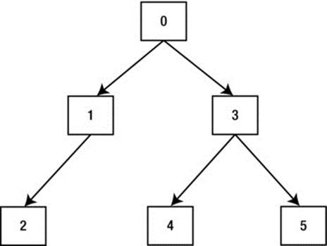
Figure 3-1. Parent-child relationships in an execution plan
Operation 0 makes one or more coroutine calls to operations 1 and 3 to generate rows, operation 1 makes coroutine calls to operation 2, and operation 3 makes coroutine calls to operations 4 and 5. The idea is that a child operation collects a small number of rows and then passes them back to its parent. If the child operation isn’t complete it waits to be called again to continue.
THE CONCEPT OF COROUTINES
You may be comfortable with the concept of subroutine calls but be less comfortable with the concept of coroutines. If this is the case then it may help to do some background reading on coroutines, as this may help you understand execution plans better.
Let me go through the specific operations in Listing 3-1 the way the runtime engine would.
Operation 0: SELECT STATEMENT
The runtime engine begins with the SELECT STATEMENT itself. This particular operation always has at least one child and calls the last child first. That is, it calls the child with the highest ID—in this case operation 3. It waits for the HASH JOIN to return rows, and, for each row returned, it calls operation 1 to evaluate the correlated subquery in the select list. Operation 1 adds the extra column, and the now complete row is output. If the HASH JOIN isn’t finished it is called again to retrieve more rows.
Operation 1: SORT AGGREGATE
Operations 1 and 2 relate to the correlated subquery in the select list. I have highlighted the correlated subquery and the associated operations in Listing 3-1. Operation 1 is called multiple times during the course of the SQL statement execution and on each occasion is passed as input theDEPTNO from the main query. It calls its child, operation 2, passing the DEPTNO parameter, to perform a TABLE ACCESS FULL and pass rows back. All SORT AGGREGATE does is to count these rows and discard them. When the count has been returned it passes its single-row, single-column output to its parent: operation 0. You can see that the estimated cardinality for this operation is 1, which confirms the understanding of this operation’s function.
Operation 2: TABLE ACCESS FULL
Because operation 1 is called multiple times during the course of the SQL statement and operation 1 always calls operation 2 once, operation 2 is called multiple times throughout the course of the statement as well. It performs a TABLE ACCESS FULL on each occasion. As rows are returned from the operation, but before being returned to operation 1, the filter predicate is applied; the DEPTNO from the row is matched with the DEPTNO input parameter, and the row is discarded if it does not match.
Operation 3: HASH JOIN
This operation performs a join of the EMP and DEPT columns. The operation starts off by calling its first child, operation 4, and as rows are returned they are placed into an in-memory hash cluster. Once all rows from DEPT have been returned and operation 4 is complete, operation 5 begins. As rows from operation 5 are returned they are matched with rows returned from operation 4, and, assuming one or more rows match, they are returned to operation 0 for further processing. In the case of a HASH JOIN (or any join for that matter) there are always exactly two child operations, and they are each invoked once per invocation of the join.
Operations 4 and 5: TABLE FULL SCANs
These operations perform full table scans on the EMP and DEPT tables and just pass their results back to their parent, operation 3. There are no predicates on these operations and, in this case, no child operations.
How Operations Interact Wrap Up
You can see that in reality there are multiple operations in progress at any one time. As rows are returned from operation 5 they are joined by operation 3 and passed back to operation 0 that then invokes operation 1, and indirectly operation 2 as well. The “topmost innermost” operation is operation 2, which was the last to start and almost the last to finish, so that blows that theory.
How Long Do Operations Take?
I have to balance being emphatic with nagging, but let me remind you again that at this stage I am just talking about how long the CBO thinks that operations will take to run, not how long they actually take to run in practice. Even the figures presented fromDBMS_XPLAN.DISPLAY_CURSOR and DBMS_XPLAN.DISPLAY_AWR are still the initial estimates (in the default display) rather than the actual elapsed times. Much of the job of analyzing SQL statement performance lies in identifying the difference between the initial estimates and the reality in practice. I’ll come onto identifying the actual cardinalities and runtimes in Chapter 4.
I have already stated that the cardinality estimate (the column with heading “rows”) is based upon a single invocation. The cost and time columns are also based on single invocations. If you look at Listing 3-1 again you will see that the cost for operation 2 and operation 5 are the same despite the fact that operation 2 is invoked multiple times and operation 5 just once. I am not sure why the figures are presented in this way, but there it is.
INLIST ITERATOR AND PARTITION RANGE OPERATIONS
One of the reasons it is so difficult to explain how to read an execution plan is that there are so many exceptions. In the case of the INLIST ITERATOR and the PARTITION RANGE operators, the rows, bytes, cost, and time columns reported by the child operation (in fact all descendants) reflect the accumulated cost of all invocations rather than those of individual calls.
The cost/time for a parent operation includes the cost of its child operations. So in Listing 3-1 you can see that the cost of operation 3 is 7, while the cost of its two child operations, 4 and 5, are 3 each. This means that the HASH JOIN itself is expected to have an overhead of 1 (all CPU it seems…that makes sense).
But hold on. The SELECT STATEMENT itself has a cost of 7. Where has the cost of the subqueries disappeared to? These have a cost of 3 each, and the runtime engine does several of them. This is simply a bug. If you want to see another bug take a look at the CPU percentages reported for the costs of operation 0 in Listings 3-2 and 3-3. These are 100%, and for operation 0 they are always 100% in the case of DBMS_XPLAN.DISPLAY_CURSOR and DBMS_XPLAN.DISPLAY_AWR. These sorts of anomalies abound, and I only point these issues out because when you first try to understand execution plans you are likely to assume that these anomalies reflect a fundamental lack of understanding on your part. Not in these cases.
Summary
In this chapter I have introduced, with examples, the techniques for displaying and interpreting some simple SQL statements with basic formatting. Even with these simple examples there is a lot still left unexplained, but some of these questions will be answered when I have covered a few more concepts.
The good news is that much of the anomalous behavior that we see when looking at the CBO’s initial estimates disappears when we look at actual statistics produced by the runtime engine. So let us get on with that in Chapter 4.