Oracle Database 12c DBA Handbook (2015)

In Chapter 6, we talked about bigfile tablespaces and how they not only allow the total size of the database to be much larger than in previous versions of Oracle, but also ease administration by moving the maintenance point from the datafile to the tablespace.

In Chapter 4, I presented an overview of Automatic Storage Management (ASM) and how it can ease administration, enhance performance, and improve availability. The DBA can add one or more disk volumes to a rapidly growing database without bringing down the instance.

In this chapter, we’ll revisit many of these database features, but with an emphasis on how they can be leveraged in a VLDB (Very Large Database) environment. Although these features surely provide benefits in all Oracle installations, they are especially useful in databases whose most heavily used resource is the amount of disk space allocated. First, we’ll review the concepts behind bigfile tablespaces and delve more deeply into how they are constructed using a new ROWID format. I’ll also show how transportable tablespaces are a distinct advantage in a VLDB environment because they bypass some of the export/import steps required in versions prior to Oracle9i to move the contents of a tablespace from one database to another. When tablespaces in a VLDB environment approach the exabyte size, both the extra space required for a traditional export and import operation and the time it takes to perform the export may become prohibitive. If you are using Oracle Database 11g or Oracle Database 12c, your tablespaces may even be transportable between different hardware and software platforms with minimal or no extra effort.

Next, we will review the various types of nontraditional (non-heap-based) tables that are often leveraged in a VLDB environment. Index-organized tables (IOTs) combine the best features of a traditional table with the fast access of an index into one segment; we’ll review some examples of how IOTs can now be partitioned in Oracle 12c. Global temporary tables dramatically reduce space usage in the undo tablespace and redo logs for recovery purposes because the table contents only persist for the duration of a transaction or a session. External tables make it easy to access data in a non-Oracle format as if the data was in a table; as of Oracle 10g, external tables can be created using Oracle Data Pump (see Chapter 13 for an in-depth discussion of Data Pump). Finally, the amount of space occupied by a table can be dramatically reduced by using an internal compression algorithm when the rows are loaded using direct-path SQL*Loader and CREATE TABLE AS SELECT statements.

Table and index partitioning not only improves query performance but tremendously improves the manageability of tables in a VLDB environment by allowing you to perform maintenance operations on one partition while users may be accessing other partitions of the table. We will cover all the different types of partitioning schemes, including some of the partitioning features first introduced in Oracle 10g: hash-partitioned global indexes, list-partitioned IOTs, and LOB support in all types of partitioned IOTs. Oracle 11g brought even more partitioning options to the table: composite list-hash, list-list, list-range, and range-range. Other new partitioning schemes in Oracle Database 11g and Oracle Database 12c include automated interval partitioning, reference partitioning, application-controlled partitioning, and virtual column partitioning.

Bitmap indexes, available since Oracle 7.3, provide query benefits not only for tables with columns of low cardinality, but also for special indexes called bitmap join indexes that pre-join two or more tables on one or more columns. Oracle 10g removed one of the remaining obstacles for using bitmap indexes in a heavy, single-row insert, update, or delete environment: mitigating performance problems due to bitmap index fragmentation issues.

Creating Tablespaces in a VLDB Environment

The considerations for creating tablespaces in a small database (terabyte range or smaller) also apply to VLDBs: Spread out I/O across multiple devices, use a logical volume manager (LVM) with RAID capabilities, or use ASM. In this section, I will present more detail and examples for bigfile tablespaces. Because a bigfile tablespace contains only one datafile, the ROWID format for objects stored in a bigfile tablespace is different, allowing for a tablespace size as large as eight million terabytes, depending on the tablespace’s block size.

Bigfile tablespaces are best suited for an environment that uses ASM, Oracle Managed Files (OMF), and Recovery Manager (RMAN) with a fast recovery area. See Chapter 6 for a detailed review of ASM; Chapter 14 presents RMAN from a command-line and Enterprise Manager Cloud Control perspective and leverages the fast recovery area for all backups. Finally, Chapter 6 describes OMF from a space-management perspective.

In the next few sections, I will present an in-depth look at creating a bigfile tablespace and specifying its characteristics; in addition, I will discuss the impact of bigfile tablespaces on both initialization parameters and data dictionary views. Finally, I will show you how the DBVERIFY utility has been revised as of Oracle 10g to allow you to analyze a single bigfile datafile using parallel processes.

Bigfile Tablespace Basics

Using bigfile tablespaces with a block size of 32KB, a datafile can be as large as 128 terabytes, with a maximum database size of 8 exabytes (EB). In contrast, a database using only smallfile tablespaces can have a maximum datafile size of 128 gigabytes (GB) and therefore a maximum database size of 8 petabytes (PB). Because a bigfile tablespace can only have one datafile, you never need to decide whether to add a datafile to the single datafile for the tablespace; once you turn on AUTOEXTEND, the single datafile will only increase in size at the increment you specify. If you are using ASM and OMF, you won’t even need to know the name of the single datafile.

Given that the maximum number of datafiles in a database on most platforms is 65,533, and the number of blocks in a bigfile tablespace datafile is 2³², you can calculate the maximum amount of space (M) in a single Oracle database as the maximum number of datafiles (D) multiplied by the maximum number of blocks per datafile (F) multiplied by the tablespace block size (B):

M = D * F * B

Therefore, the maximum database size, given the maximum block size and the maximum number of datafiles, is

65,533 datafiles * 4,294,967,296 blocks per datafile * 32,768 block size = 9,223,231,299,366,420,480 = 8EB

For a smallfile tablespace, the number of blocks in a smallfile tablespace datafile is only 2²². Therefore, our calculation yields

65,535 datafiles * 4,194,304 blocks per datafile * 32,768 block size = 9,007,061,815,787,520 = 8PB

In Table 18-1, you can see a comparison of maximum datafile sizes for smallfile tablespaces and bigfile tablespaces given the tablespace block size. If for some reason your database size approaches 8EB, you may want to consider either some table archiving or splitting the database into multiple databases based on function. With even the largest commercial Oracle databases in the petabyte (PB) range in 2015, you may very well not bump up against the 8EB limit any time in the near future!

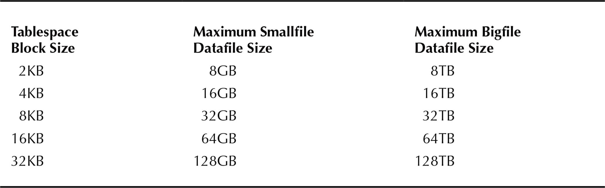
TABLE 18-1. Maximum Tablespace Datafile Sizes

Creating and Modifying Bigfile Tablespaces

Here is an example of creating a bigfile tablespace in a non-ASM environment:

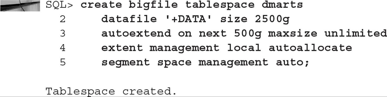
In the example, you can see that EXTENT MANAGEMENT and SEGMENT SPACE MANAGEMENT are explicitly set, even though AUTO is the default for segment space management; bigfile tablespaces must be created as locally managed with automatic segment space management. Because the default allocation policy for both bigfile and smallfile tablespaces is AUTOALLOCATE, you don’t need to specify it either. As a rule of thumb, AUTOALLOCATE is best for tablespaces whose table usage and growth patterns are indeterminate; as I’ve pointed out in Chapter 6, you use UNIFORM extent management only if you know the precise amount of space you need for each object in the tablespace as well as the number and size of extents.

Even though the datafile for this bigfile tablespace is set to autoextend indefinitely, the disk volume where the datafile resides may be limited in space; when this occurs, the tablespace may need to be relocated to a different disk volume. Therefore, you can see the advantages of using ASM: You can easily add another disk volume to the disk group where the datafile resides, and Oracle will automatically redistribute the contents of the datafile and allow the tablespace to grow—all of this occurring while the database (and the tablespace itself) is available to users.

By default, tablespaces are created as smallfile tablespaces; you can specify the default tablespace type when the database is created or at any time with the ALTER DATABASE command, as in this example:

Bigfile Tablespace ROWID Format

To facilitate the larger address space for bigfile tablespaces, a new extended ROWID format is used for rows of tables in bigfile tablespaces. First, we will review the ROWID format for smallfile tablespaces in previous versions of Oracle and for Oracle 12c. The format for a smallfile ROWID consists of four parts:

Table 18-2 defines each part of a smallfile ROWID.

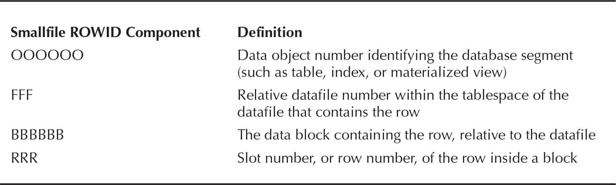
TABLE 18-2. Smallfile ROWID Format

In contrast, a bigfile tablespace only has one datafile, and its relative datafile number is always 1024. Because the relative datafile number is fixed, it is not needed as part of the ROWID; as a result, the part of the ROWID used for the relative datafile number can be used to expand the size of the block number field. The concatenation of the smallfile relative datafile number (FFF) and the smallfile data block number (BBBBBB) results in a new construct called an encoded block number. Therefore, the format for a bigfile ROWID consists of only three parts:

Table 18-3 defines each part of a bigfile ROWID.

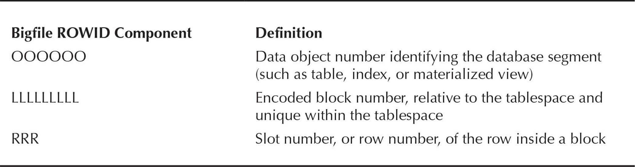
TABLE 18-3. Bigfile ROWID Format

DBMS_ROWID and Bigfile Tablespaces

Because two different types of tablespaces can now coexist in the database along with their corresponding ROWID formats, some changes have occurred to the DBMS_ROWID package.

The names of the procedures in the DBMS_ROWID package are the same and operate as before, except for a new parameter, TS_TYPE_IN, which identifies the type of tablespace to which a particular row belongs: TS_TYPE_IN can be either BIGFILE or SMALLFILE.

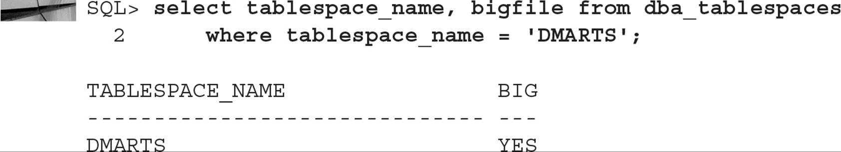
For an example of extracting ROWIDs from a table in a bigfile tablespace, we have a table called OE.ARCH_ORDERS in a bigfile tablespace named DMARTS:

As with tables in smallfile tablespaces in previous versions of Oracle and in Oracle 12c, we can use the pseudo-column ROWID to extract the entire ROWID, noting that the format of the ROWID is different for bigfile tables, even though the length of the ROWID stays the same. This query will also extract the block number in decimal format:

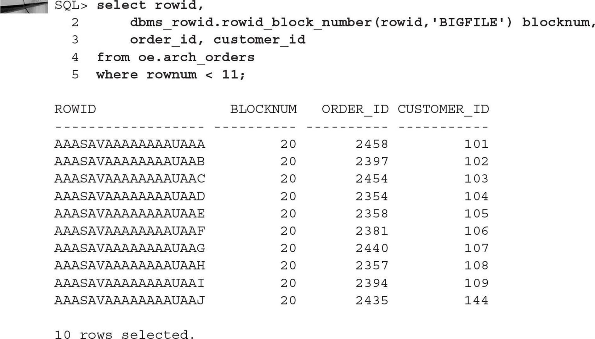
For the row with the ORDER_ID of 2358, the data object number is AAASAV, the encoded block number is AAAAAAAAU, and the row number of the row, or slot, in the block is AAE; the translated decimal block number is 20.

NOTE

ROWIDs use base-64 encoding.

The other procedures in the DBMS_ROWID package that use the variable TS_TYPE_IN to specify the tablespace type are ROWID_INFO and ROWID_RELATIVE_FNO.

The procedure ROWID_INFO returns five attributes for the specified ROWID via output parameters. In Table 18-4 you can see the parameters of the ROWID_INFO procedure.

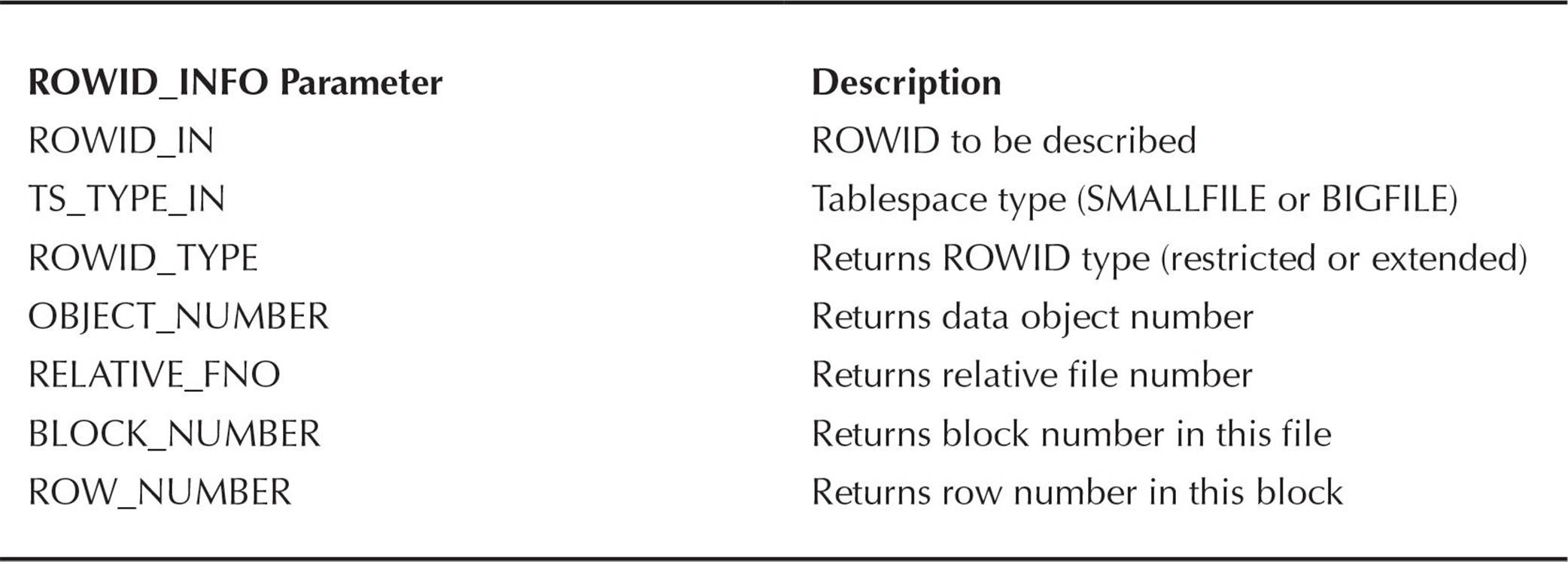
TABLE 18-4. ROWID_INFO Parameters

In the following example, we’ll use an anonymous PL/SQL block to extract the values for OBJECT_NUMBER, RELATIVE_FNO, BLOCK_NUMBER, and ROW_NUMBER for a row in the table OE.ARCH_ORDERS:

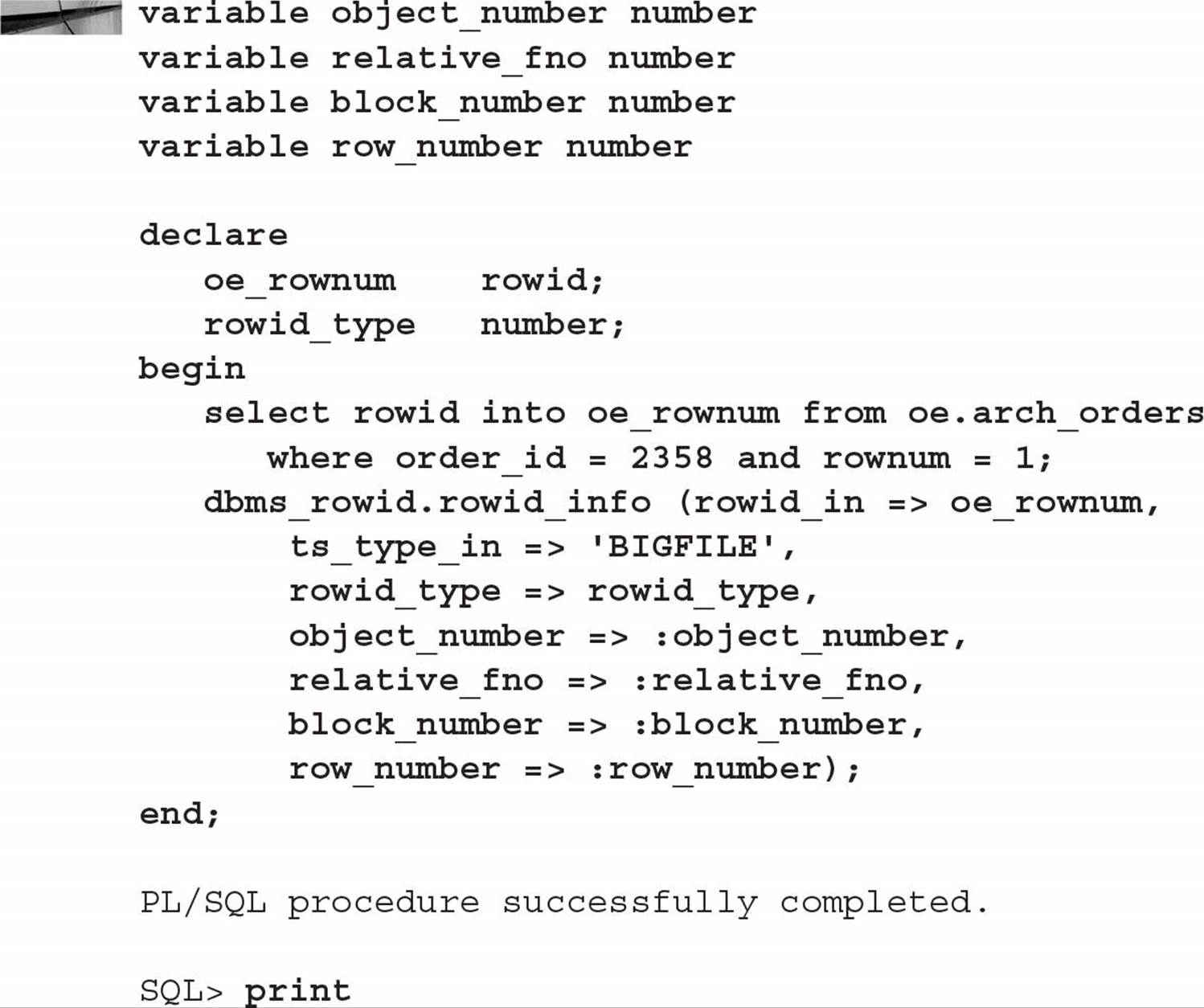
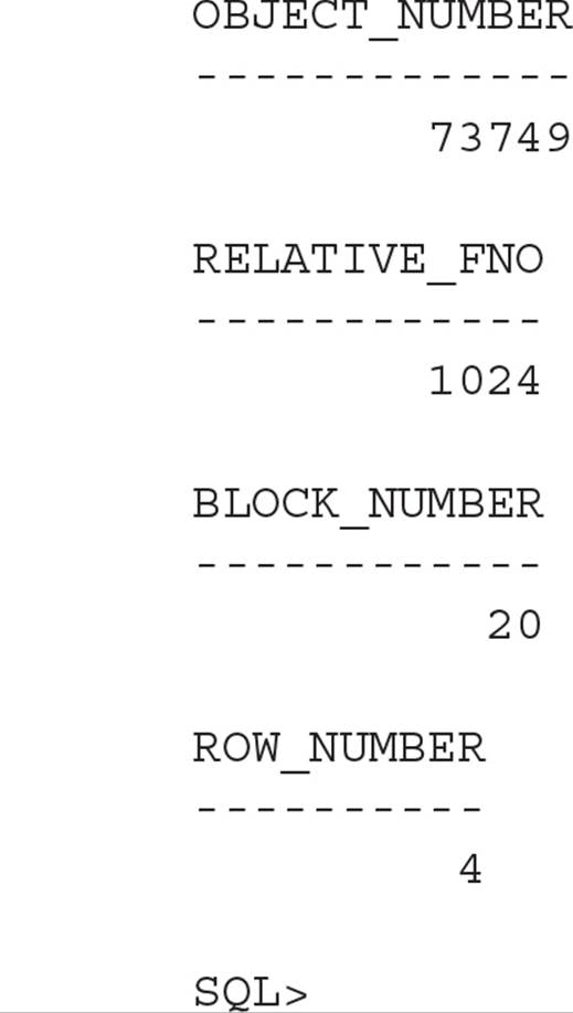
Note that the return value for RELATIVE_FNO is always 1024 for a bigfile tablespace, and the BLOCK_NUMBER is 20, as you saw in the previous example that used the DBMS_ROWID.ROWID_BLOCK_NUMBER function.

Using DBVERIFY with Bigfile Tablespaces

The DBVERIFY utility, available since Oracle version 7.3, checks the logical integrity of an offline or online database. The files can only be datafiles; DBVERIFY cannot analyze online redo log files or archived redo log files. In previous versions of Oracle, DBVERIFY could analyze all of a tablespace’s datafiles in parallel by spawning multiple DBVERIFY commands. However, because a bigfile tablespace has only one datafile, DBVERIFY has been enhanced to analyze parts of a bigfile tablespace’s datafiles in parallel.

Using the dbv command at the Unix or Windows prompt, you can use two new parameters: START and END, representing the first and last block, respectively, of the file to analyze. As a result, you need to know how many blocks are in the bigfile tablespace’s datafile; the dynamic performance view V$DATAFILE comes to the rescue, as you can see in the following example:

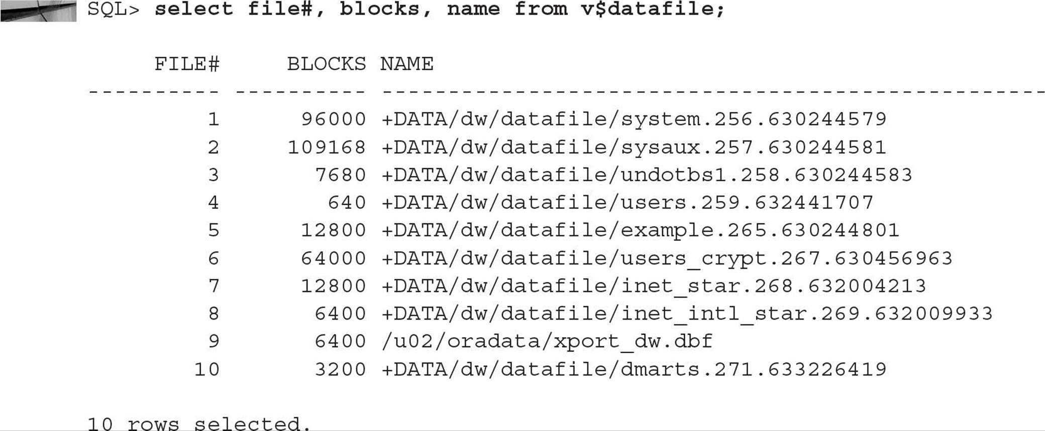
In the next example, you will see how to analyze datafile #9, the datafile for another bigfile tablespace in our database, XPORT_DW. At the operating system command prompt, you can analyze the file with five parallel processes, each processing 500 blocks, except for the last one:

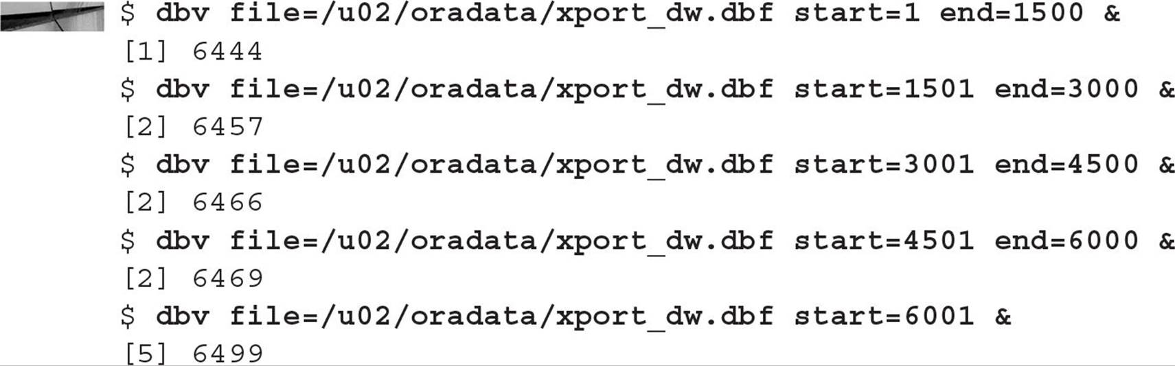
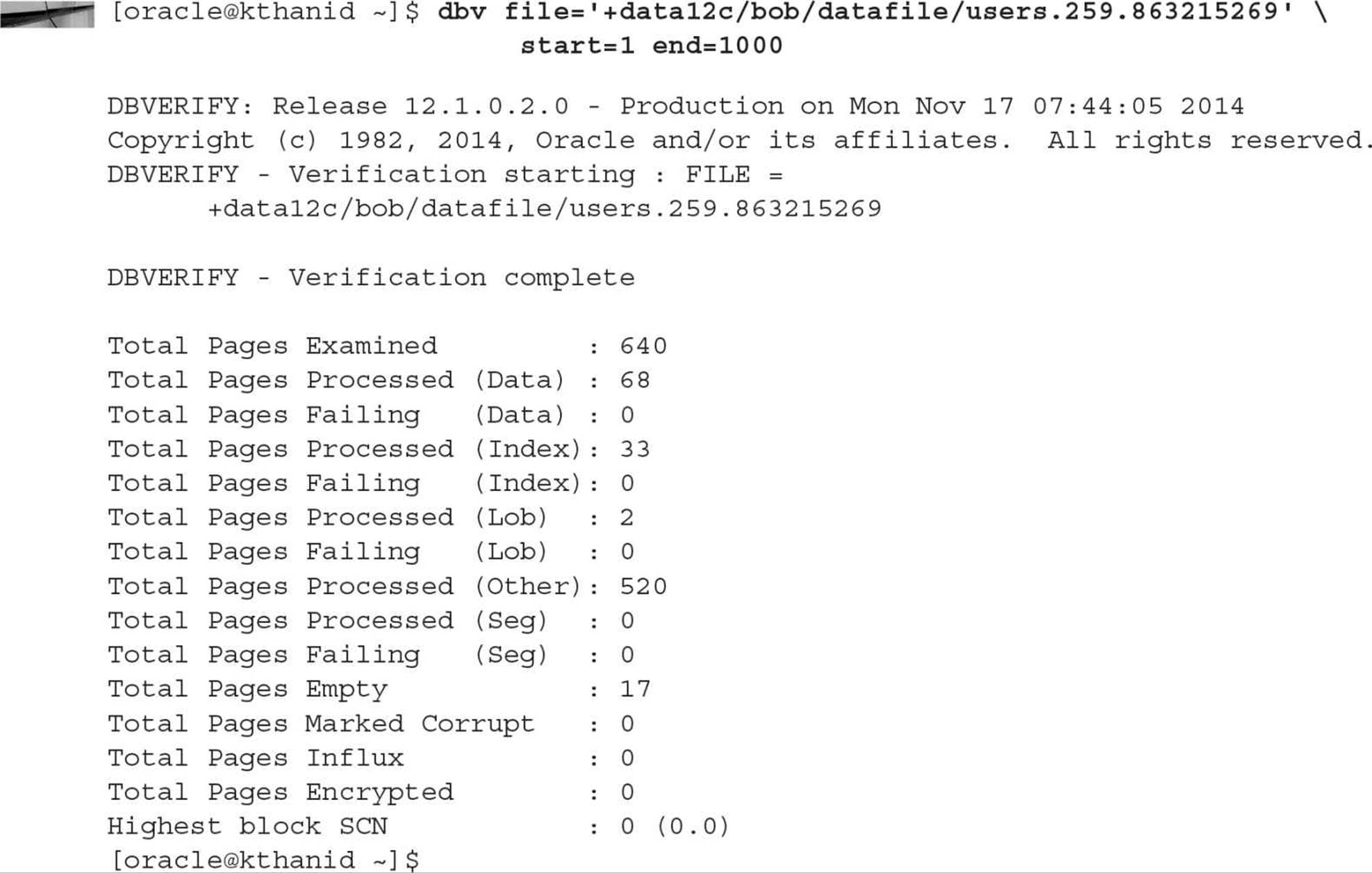
In the fifth command, we did not specify end=; if you do not specify end=, it is assumed that you will be analyzing the datafile from the starting point to the end of the file. All five of these commands run in parallel. You can also run DBVERIFY against datafiles in ASM disk groups, as in this example:

Bigfile Tablespace Initialization Parameter Considerations

Although there are no new initialization parameters specific to bigfile tablespaces, the values of one initialization parameter and a CREATE DATABASE parameter can potentially be reduced because only one datafile is needed for each bigfile tablespace. The initialization parameter is DB_FILES, and the CREATE DATABASE parameter is MAXDATAFILES.

DB_FILES and Bigfile Tablespaces

As you already know, DB_FILES is the maximum number of datafiles that can be opened for this database. If you use bigfile tablespaces instead of smallfile tablespaces, the value of this parameter can be lower; as a result, because there are fewer datafiles to maintain, memory requirements are a bit lower in the System Global Area (SGA).

MAXDATAFILES and Bigfile Tablespaces

When creating a new database or a new control file, you can use the MAXDATAFILES parameter to control the size of the control file section allocated to maintain information about datafiles. Using bigfile tablespaces, you can make the size of the control file and the space needed in the SGA for datafile information smaller; more importantly, the same value for MAXDATAFILES using bigfile tablespaces means that the total database size can be larger.

Bigfile Tablespace Data Dictionary Changes

The changes to data dictionary views due to bigfile tablespaces include a new row in DATABASE_PROPERTIES and a new column in DBA_TABLESPACES and USER_TABLESPACES.

DATABASE_PROPERTIES and Bigfile Tablespaces

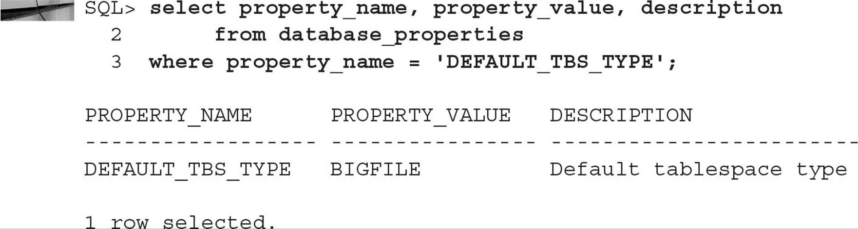
The data dictionary view DATABASE_PROPERTIES, as the name implies, contains a number of characteristics about the database, such as the names of the default and permanent tablespaces and various National Language Settings (NLS). Because of bigfile tablespaces, there is a new property in DATABASE_PROPERTIES called DEFAULT_TBS_TYPE that indicates the default tablespace type for the database if no type is specified in a CREATE TABLESPACE command. In the following example, you can find out the default new tablespace type:

*_TABLESPACES, V$TABLESPACE, and Bigfile Tablespaces

The data dictionary views DBA_TABLESPACES and USER_TABLESPACES have a new column called BIGFILE. The value of this column is YES if the corresponding tablespace is a bigfile tablespace, as you saw in the query against DBA_TABLESPACES earlier in this chapter. The dynamic performance view V$TABLESPACE also contains this column.

Advanced Oracle Table Types

Many other table types provide benefits in a VLDB environment. Index-organized tables, for example, eliminate the need for both a table and its corresponding index, replacing them with a single structure that looks like an index but contains data like a table. Global temporary tables create a common table definition available to all database users; in a VLDB, a global temporary table shared by thousands of users is preferable to each user creating their own definition of the table, potentially putting further space pressure on the data dictionary. External tables allow you to use text-based files outside of the database without actually storing the data in an Oracle table. Partitioned tables, as the name implies, store tables and indexes in separate partitions to keep the availability of the tables high while keeping maintenance time low. Finally, materialized views preaggregate query results from a view and store the query results in a local table; queries that use the materialized view may run significantly faster because the results from executing the view do not need to be re-created. We will cover all these table types to varying levels of detail in the following sections.

Index-Organized Tables

You can store index and table data together in a table known as an index-organized table (IOT). Significant reductions in disk space are achieved with IOTs because the indexed columns are not stored twice (once in the table and once in the index); instead, they are stored once in the IOT along with any non-indexed columns. IOTs are suitable for tables where the primary access method is through the primary key, although creating indexes on other columns of the IOT is allowed, to improve access by those columns.

In the following example, you will create an IOT with a two-part (composite) primary key:

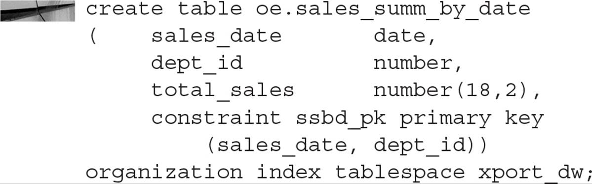
Each entry in the IOT contains a date, a department number, and a total sales amount for the day. All three of these columns are stored in each IOT row, but the IOT is built based on only the date and department number. Only one segment is used to store an IOT; if you build a secondary index on this IOT, a new segment is created.

Because the entire row in an IOT is stored as the index itself, there is no ROWID for each row; the primary key identifies the rows in an IOT. Instead, Oracle creates logical ROWIDs derived from the value of the primary key; the logical ROWID is used to support secondary indexes on the IOT.

If you still want to use an IOT for a frequently accessed set of columns but also include a number of infrequently accessed non-indexed columns, you can include these columns in an overflow segment by specifying the INCLUDING and OVERFLOW TABLESPACE clauses as in this example:

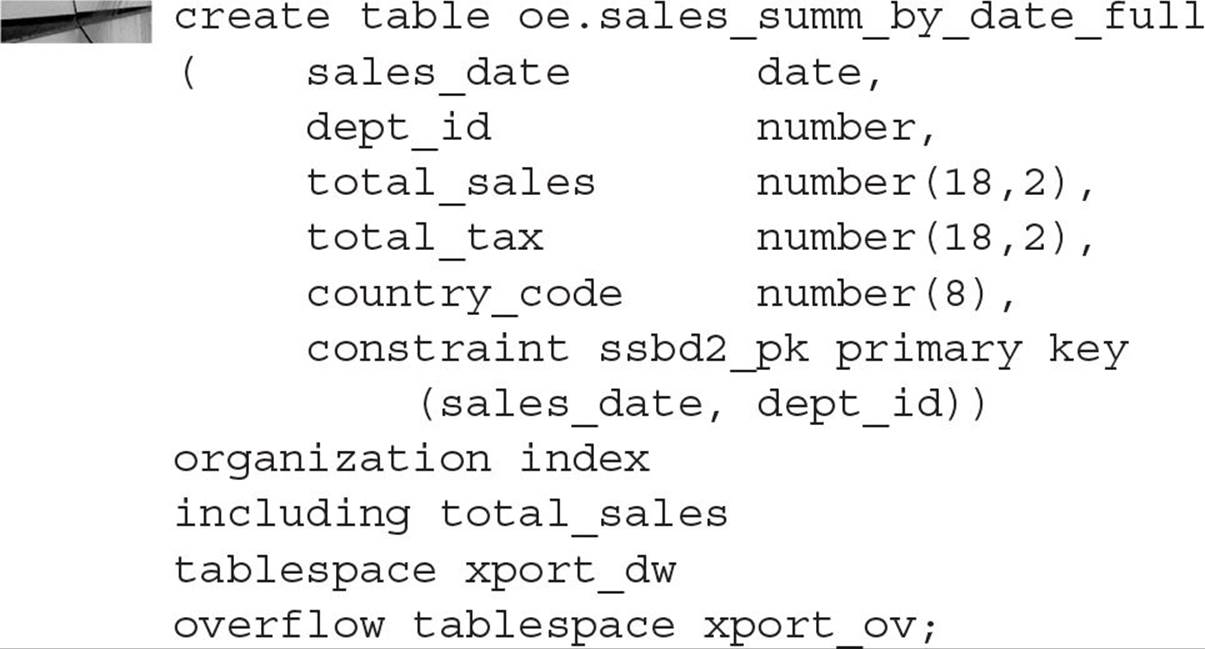
The columns starting with TOTAL_TAX will be stored in an overflow segment in the XPORT_OV tablespace.

No special syntax is required to use an IOT; although it is built and maintained much like an index, it appears as a table to any SQL SELECT statement or other DML statements. Also, IOTs can be partitioned; information about partitioning IOTs is presented later in this chapter, in the section “Partitioned Index-Organized Tables.”

Global Temporary Tables

Temporary tables have been available since Oracle8i. They are temporary in the sense of the data that is stored in the table, not in the definition of the table itself. The command CREATE GLOBAL TEMPORARY TABLE creates a temporary table; all users who have permissions on the table itself can perform DML on a temporary table. However, each user sees their own and only their own data in the table. When a user truncates a temporary table, only the data that they inserted is removed from the table. Global temporary tables are useful in situations where a large number of users need a table to hold temporary data for their session or transaction, while only needing one definition of the table in the data dictionary. Global temporary tables have the added advantage of reducing the need for redo or undo space for the entries in the table in a recovery scenario. The entries in a global temporary table, by their nature, are not permanent and therefore do not need to be recovered during instance or media recovery.

There are two different flavors of temporary data in a temporary table: temporary for the duration of the transaction, and temporary for the duration of the session. The longevity of the temporary data is controlled by the ON COMMIT clause; ON COMMIT DELETE ROWS removes all rows from the temporary table when a COMMIT or ROLLBACK is issued, and ON COMMIT PRESERVE ROWS keeps the rows in the table beyond the transaction boundary. However, when the user’s session is terminated, all of the user’s rows in the temporary table are removed.

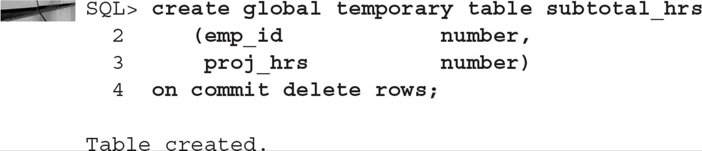
In the following example, you create a global temporary table to hold some intermediate totals for the duration of the transaction. Here is the SQL command to create the table:

For the purposes of this example, you will create a permanent table that holds the total hours by employee by project for a given day. Here is the SQL command for the permanent table:

In the following scenario, you will use the global temporary table to keep the intermediate results, and at the end of the transaction, you will store the totals in the TOTAL_HOURS table. Here is the sequence of commands:

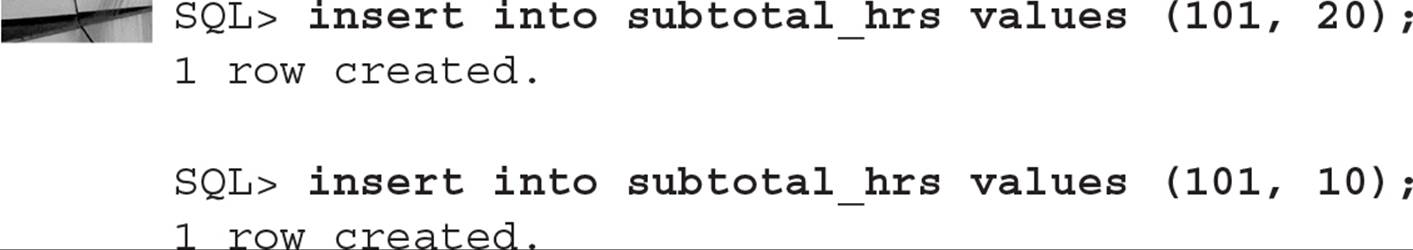
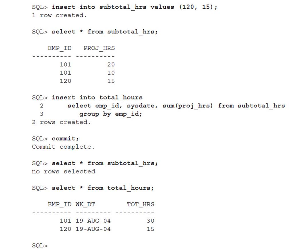
Notice that after the COMMIT, the rows are retained in TOTAL_HOURS but are not retained in SUBTOTAL_HRS because you specified ON COMMIT DELETE ROWS when you created the table.

NOTE

DDL can be performed on a global temporary table as long as there are no sessions currently inserting rows into the global temporary table.

There are a few other things to keep in mind when using temporary tables. Although you can create an index on a temporary table, the entries in the index are dropped along with the data rows, as with a regular table. Also, due to the temporary nature of the data in a temporary table, no recovery-related redo information is generated for DML on temporary tables; however, undo information is created in the undo tablespace and redo information to protect the undo. If all you do is insert and select from your global temporary tables, very little redo is generated. Because the table definition itself is not temporary, it persists between sessions until it is explicitly dropped.

As of Oracle Database 12c, statistics on a global temporary table can be specific to a session. This is important for global temporary tables whose contents and cardinality in one session vary widely from other sessions; in Oracle Database 11g there was only one set of statistics for a global temporary table, which made query optimization more difficult for queries containing global temporary tables.

External Tables

Sometimes you want to access data that resides outside of the database in a text format, but you want to use it as if it were a table in the database. Although you could use a utility such as SQL*Loader to load the table into the database, the data may be quite volatile or your user base’s expertise might not include executing SQL*Loader at the Windows or Unix command line.

To address these needs, you can use external tables, which are read-only tables whose definition is stored within the database but whose data stays external to the database. There are a few drawbacks to using external tables: You cannot index external tables, and you cannot execute UPDATE, INSERT, and DELETE statements against an external table. However, in a data warehouse environment where an external table is read in its entirety for a merge operation with an existing table, these drawbacks do not apply.

You might use an external table to gather employee suggestions in a web-based front end that does not have access to the production database; in this example, you will create an external table that references a text-based file containing two fields: the employee ID and the comment.

First, you must create a directory object to point to the operating system directory where the text file is stored. In this example, you will create the directory EMPL_COMMENT_DIR to reference a directory on the Unix file system, as follows:

The text file in this directory is called empl_sugg.txt, and it looks like this:

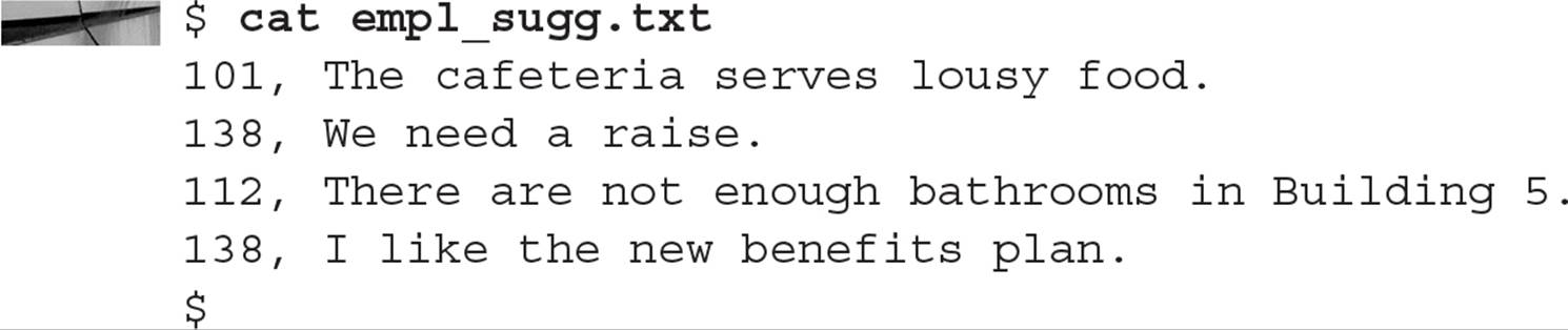
Because this text file has two fields, you will create the external table with two columns, the first being the employee number and the second being the text of the comments. Here is the CREATE TABLE command:

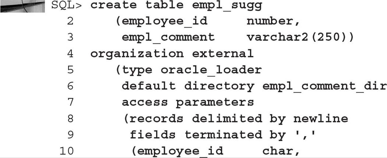
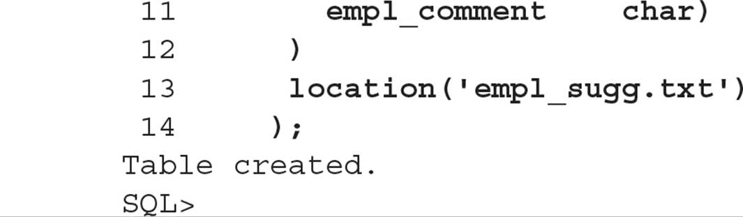
The first three lines of the command look like a standard CREATE TABLE command. The ORGANIZATION EXTERNAL clause specifies that this table’s data is stored external to the database. Using the oracle_loader clause specifies the access driver to create and to load an external table as read-only. The file specified in the LOCATION clause, empl_sugg.txt, is located in the Oracle directory empl_comment_dir, which you created earlier. The access parameters specify that each row of the table is on its own line in the text file and that the fields in the text file are separated by a comma.

NOTE

Using an access driver of oracle_datapump instead of oracle_loader allows you to unload your data to an external table; other than this initial unload, the external table is accessible for read access only through the oracle_datapump access driver and has the same restrictions as an external table created with the oracle_loader access driver.

Once the table is created, the data is immediately accessible in a SELECT statement, as if it had been loaded into a real table, as you can see in this example:

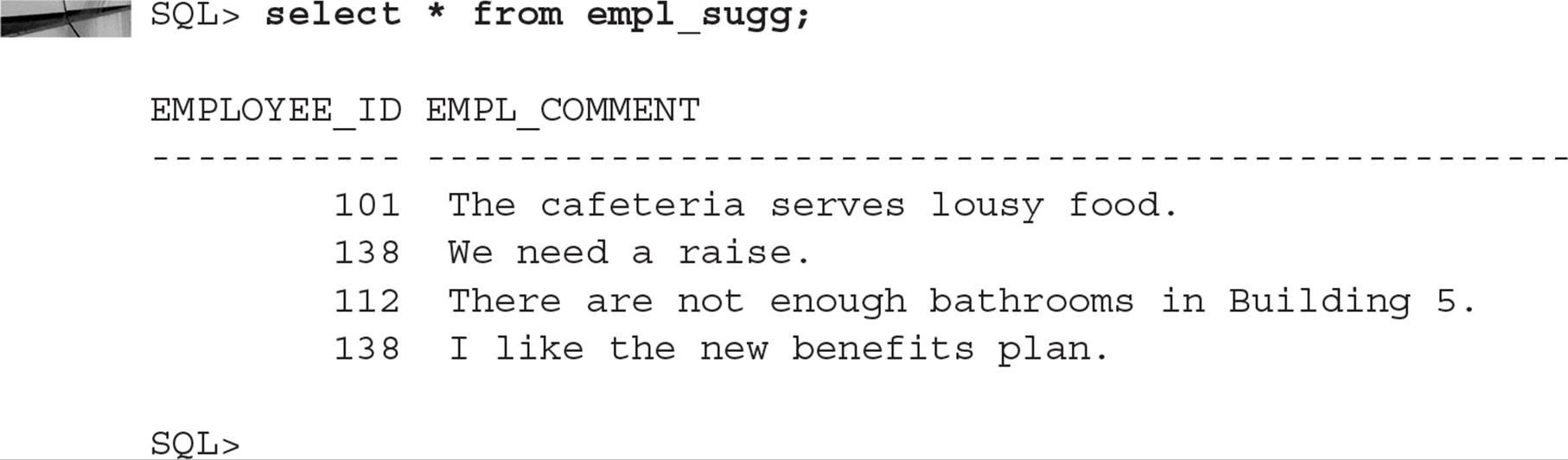
Any changes made to the text file will automatically be available the next time you execute the SELECT statement.

Partitioned Tables

In a VLDB environment, partitioned tables help to make the database more available and maintainable. A partitioned table is split up into more manageable pieces, called partitions, and can be further subdivided into subpartitions. The corresponding indexes on partitioned tables can be nonpartitioned, partitioned the same way as the table, or partitioned differently from the table.

Partitioned tables can also improve the performance of the database: Each partition of a partitioned table can be accessed using parallel execution. Multiple parallel execution servers can be assigned to different partitions of the table or to different index partitions.

For performance reasons, each partition of a table can and should reside in its own tablespace. Other attributes of a partition, such as storage characteristics, can differ; however, the column datatypes and constraints for each partition must be identical. In other words, attributes such as datatype and check constraints are at the table level, not the partition level. Other advantages of storing partitions of a partitioned table in separate tablespaces include the following:

It reduces the possibility of data corruption in more than one partition if one tablespace is damaged.

Each partition can be backed up and recovered independently.

You have more control of partition-to-physical device mapping to balance the I/O load. Even in an ASM environment, you could place each partition in a different disk group; in general, however, Oracle recommends two disk groups, one for user data and the other for flashback and recovery data. There are few reasons to limit a partition to a subset of the tens or hundreds of disks in a typical RAID-based disk group.

Partitioning is transparent to applications, and no changes to SQL statements are required to take advantage of partitioning. However, in situations where specifying a partition would be advantageous, you can specify both the table name and the partition name in a SQL statement; this improves both parse and SELECT performance. Examples of syntax using explicit partition names in a SELECT statement are found later in this chapter, in the section “Splitting, Adding, and Dropping Partitions.”

Creating Partitioned Tables

Several methods of partitioning are available in the Oracle database, and many of them were introduced in Oracle Database 10g, such as list-partitioned IOTs; other methods are new to Oracle 11g, such as composite list-hash, list-list, list-range, and range-range partitioning. In the next few sections, we’ll cover the basics of range partitioning, hash partitioning, list partitioning, six types of composite partitioning, as well as interval partitioning, reference partitioning, application-controlled partitioning, and virtual column partitioning. I’ll also show you how to selectively compress partitions within the table to save on I/O and disk space. Oracle Database 12c adds another new type of partitioning: interval-reference partitioning.

Using Range Partitioning Range partitioning is used to map rows to partitions based on ranges of one or more columns in the table being partitioned. Also, the rows to be partitioned should be fairly evenly distributed among each partition, such as by months of the year or by quarter. If the column being partitioned is skewed (for example, by population within each state code), another partitioning method may be more appropriate.

To use range partitioning, you must specify the following three criteria:

Partitioning method (range)

Partitioning column or columns

Bounds for each partition

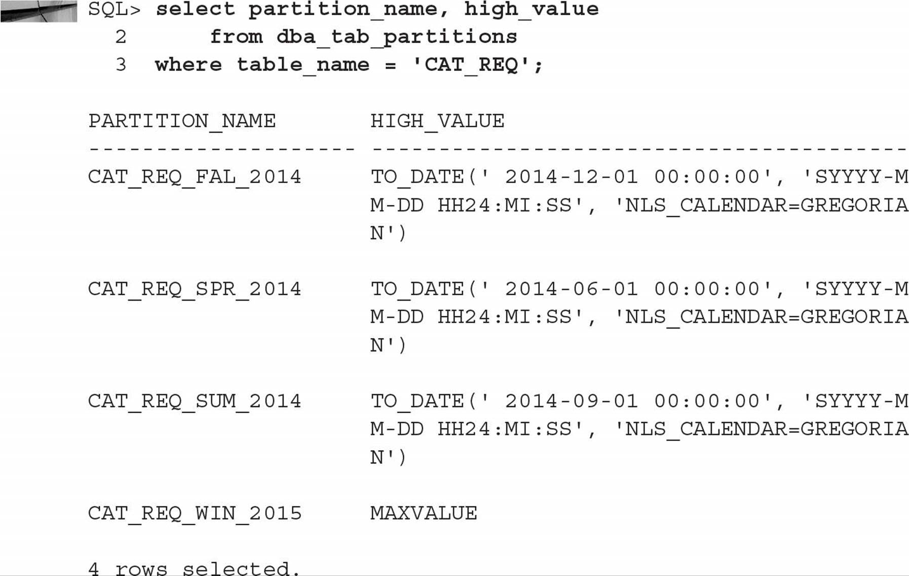
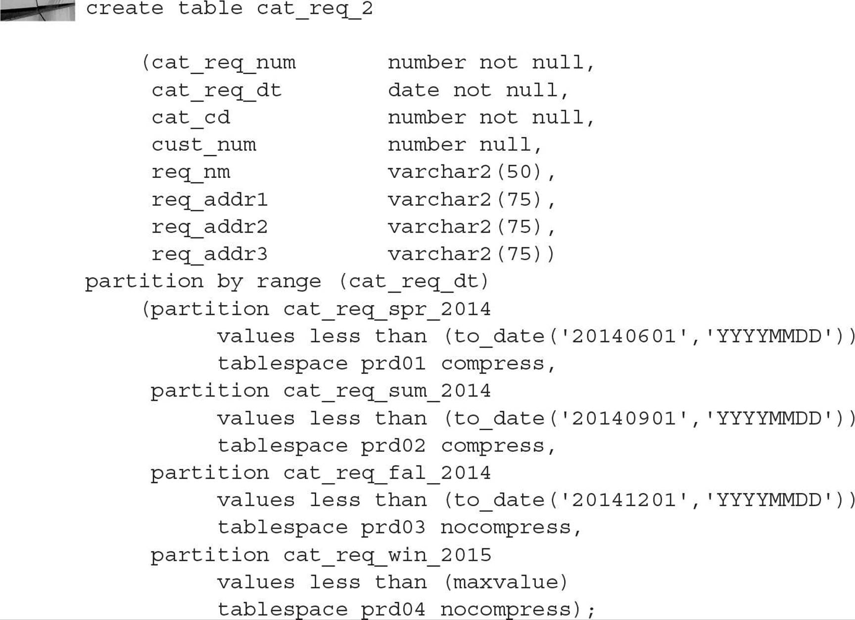
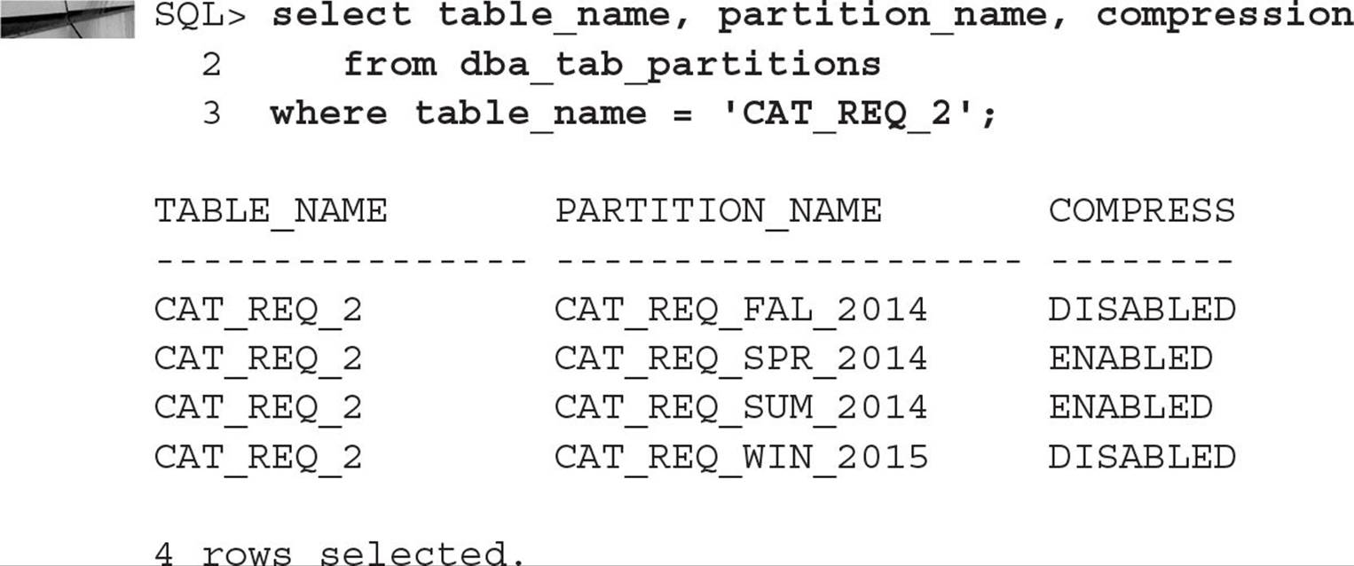
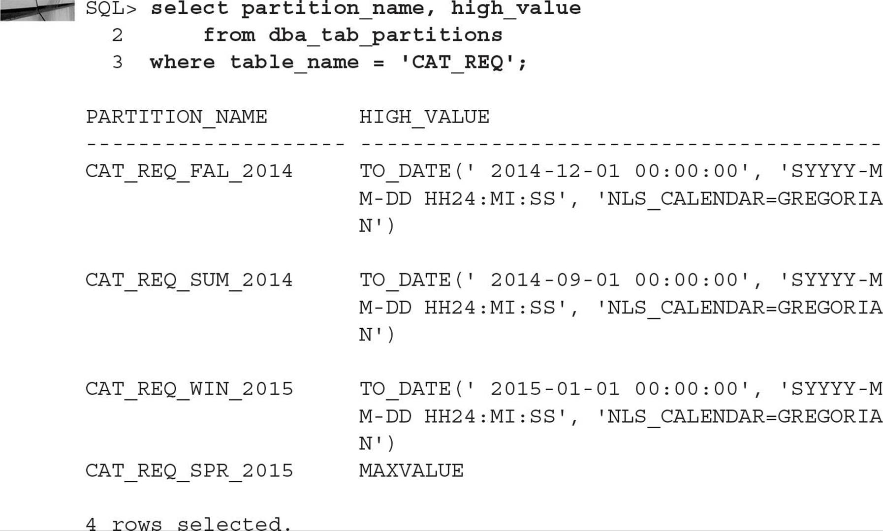
In the following example, you want to partition the catalog request table CAT_REQ by season, resulting in a total of four partitions per year:

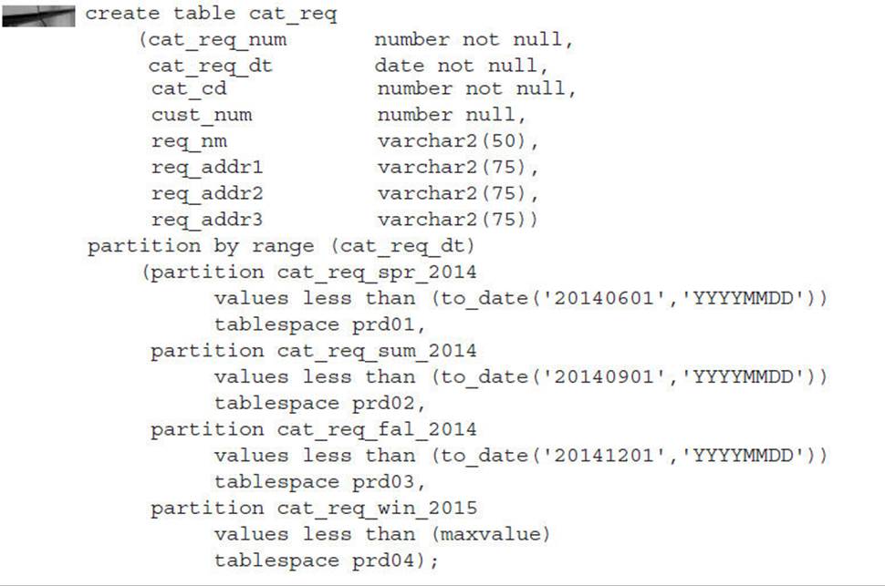
In the preceding example, the partitioning method is RANGE, the partitioning column is REQ_DATE, and the VALUES LESS THAN clause specifies the upper bound that corresponds to the dates for each season of the year: March through May (partition CAT_REQ_SPR_2014), June through August (partition CAT_REQ_SUM_2014), September through November (partition CAT_REQ_FAL_2014), and December through February (partition CAT_REQ_WIN_2015). Each partition is stored in its own tablespace—either PRD01, PRD02, PRD03, or PRD04.

You use MAXVALUE to catch any date values after 12/1/2014; if you had specified TO_DATE(‘20150301’,‘YYYYMMDD’) as the upper bound for the fourth partition, then any attempt to insert rows with date values after 2/28/2015 would fail. On the other hand, any rows inserted with dates before 6/1/2014 would end up in partition CAT_REQ_SPR_2014, even rows with a catalog request date of 10/1/1963! This is one case where the front-end application may provide some assistance in data verification, both at the low end and the high end of the date range.

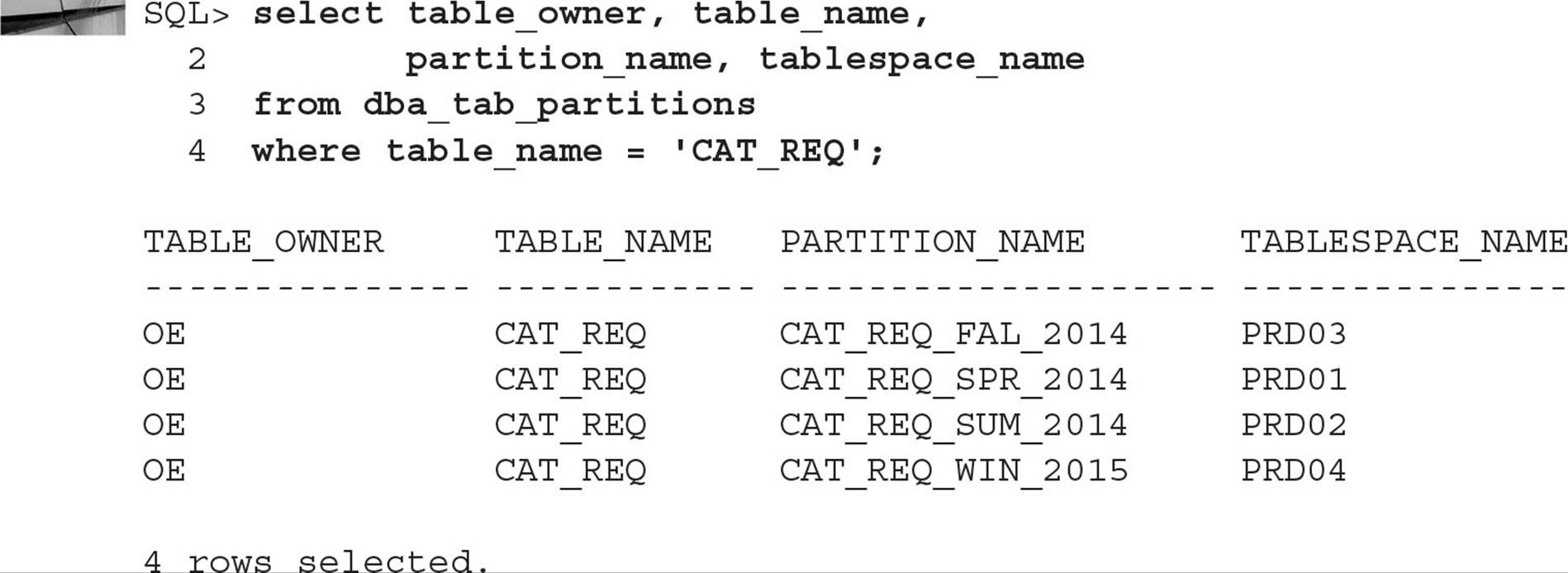
The data dictionary view DBA_TAB_PARTITIONS shows you the partition components of the CAT_REQ table, as you can see in the following query:

Finding out the dates used in the VALUES LESS THAN clause when the partitioned table was created can be done in the same data dictionary view, as you can see in the following query:

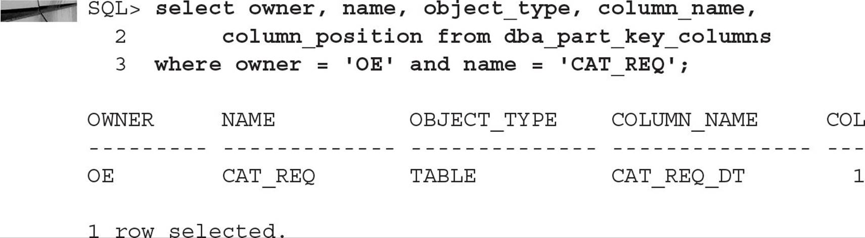
In a similar fashion, you can use the data dictionary view DBA_PART_KEY_COLUMNS to find out the columns used to partition the table, as in the following example:

I will show you how to modify the partitions of a partitioned table later in this chapter, in the section “Managing Partitions.”

Using Hash Partitioning Hash partitioning is a good option if the distribution of your data does not easily fit into a range partitioning scheme or the number of rows in the table is unknown, but you otherwise want to take advantage of the benefits inherent in partitioned tables. Rows are evenly spread out to two or more partitions based on an internal hashing algorithm using the partition key as input. The more distinct the values are in the partitioning column, the better the distribution of rows across the partitions.

To use hash partitioning, you must specify the following three criteria:

Partitioning method (hash)

Partitioning column or columns

The number of partitions and a list of target tablespaces in which to store the partitions

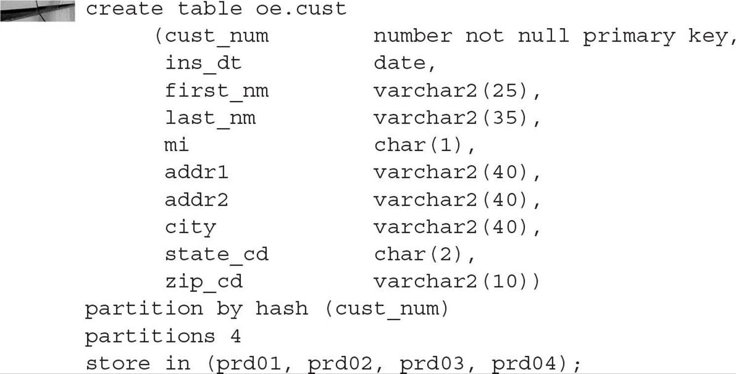
For this example, you are creating a new customer table whose primary key is generated using a sequence. You want the new rows to be evenly distributed across four partitions; therefore, hash partitioning would be the best choice. Here is the SQL you use to create a hash-partitioned table:

You do not necessarily have to specify the same number of partitions as tablespaces; if you specify more partitions than tablespaces, the tablespaces are reused for subsequent partitions in a round-robin fashion. If you specify fewer partitions than tablespaces, the extra tablespaces at the end of the tablespace list are ignored.

If you run the same queries that you ran for range partitioning, you may find some unexpected results, as you can see in this query:

Because you are using hash partitioning, the HIGH_VALUE column is NULL.

TIP

Oracle strongly recommends that the number of partitions in a hash-partitioned table be to a power of 2 to get an even distribution of rows in each table; Oracle uses the low-order bits of the partition key to determine the destination partition for the row.

Using List Partitioning List partitioning gives you explicit control of how each value in the partitioning column maps to a partition by specifying discrete values from the partitioning column. Range partitioning is usually not suitable for discrete values that do not have a natural and consecutive range of values, such as state codes. Hash partitioning is not suitable for assigning discrete values to a particular partition because, by its nature, a hash partition may map several related discrete values into different partitions.

To use list partitioning, you must specify the following three criteria:

Partitioning method (list)

Partitioning column

Partition names, with each partition associated with a discrete list of literal values that place it in the partition

NOTE

As of Oracle 10g, list partitioning can be used for tables with LOB columns.

In the following example, you will use list partitioning to record sales information for the data warehouse into three partitions based on sales region: the Midwest, the western seaboard, and the rest of the country. Here is the CREATE TABLE command:

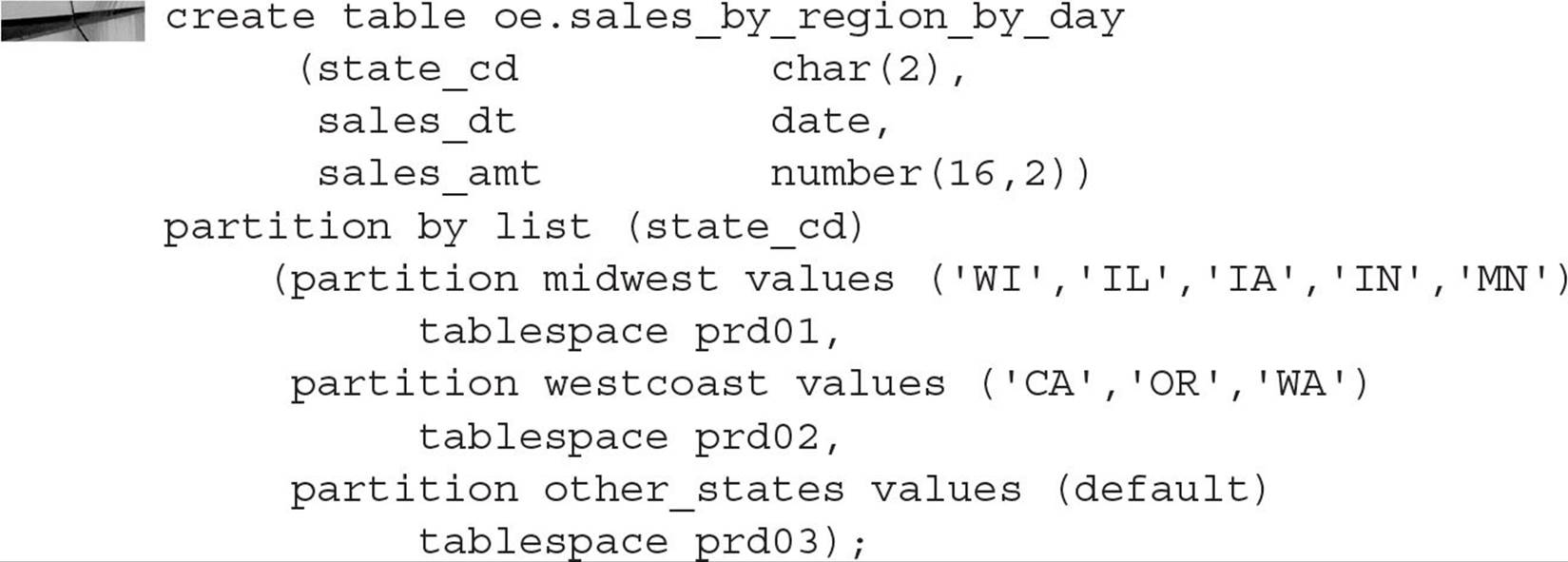
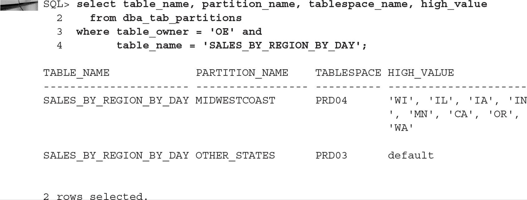
Sales information for Wisconsin, Illinois, and the other Midwestern states will be stored in the MIDWEST partition; California, Oregon, and Washington state will end up in the WESTCOAST partition. Any other value for state code, such as MI, will end up in the OTHER_STATES partition in tablespace PRD03.

Using Composite Range-Hash Partitioning As the name implies, range-hash partitioning uses range partitioning to divide rows first using the range method and then subpartitioning the rows within each range using a hash method. Composite range-hash partitioning is good for historical data with the added benefit of increased manageability and data placement within a larger number of total partitions.

To use composite range-hash partitioning, you must specify the following criteria:

Primary partitioning method (range)

Range partitioning column(s)

Partition names identifying the bounds of the partition

Subpartitioning method (hash)

Subpartitioning column(s)

Number of subpartitions for each partition or subpartition name

In the following example, you will track house and garden tool rentals. Each tool is identified by a unique tool number; at any given time, only about 400 tools are available for rental, although there may be slightly more than 400 on a temporary basis. For each partition, you want to use hash partitioning for each of eight subpartitions, using the tool name in the hashing algorithm. The subpartitions will be spread out over four tablespaces: PRD01, PRD02, PRD03, and PRD04. Here is the CREATE TABLE command to create the range-hash partitioned table:

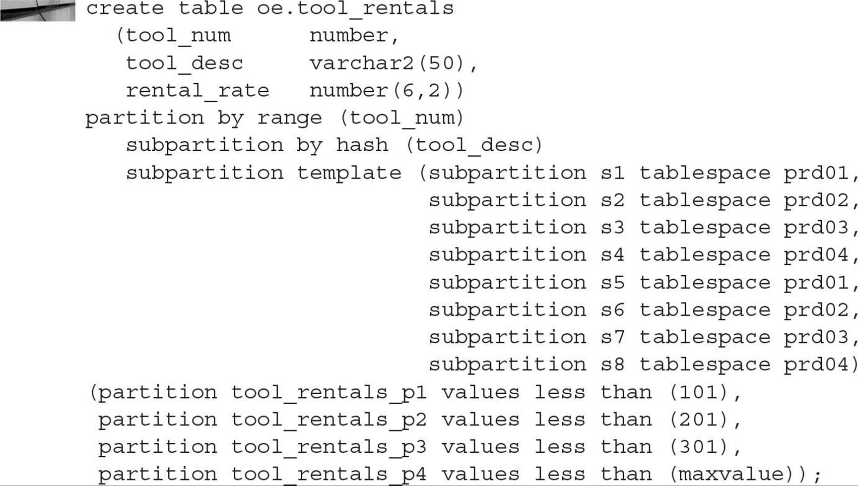
The range partitions are logical only; there are a total of 32 physical partitions, one for each combination of logical partition and subpartition in the template list. Note the SUBPARTITION TEMPLATE clause; the template is used for creating the subpartitions in every partition that doesn’t have an explicit subpartition specification. It can be a real timesaver and reduce typing errors if the subpartitions are explicitly specified for each partition. Alternatively, you could specify the following clause, if you do not need the subpartitions explicitly named:

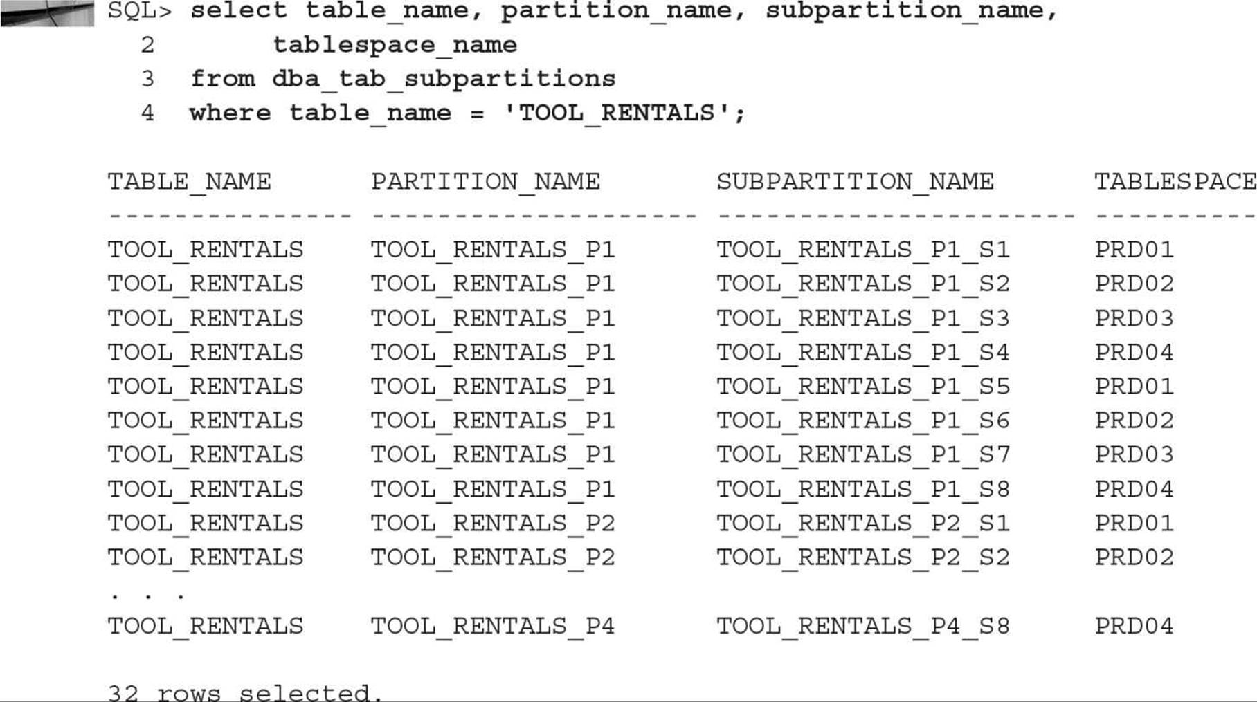
The physical partition information is available in DBA_TAB_SUBPARTITIONS, as for any partitioned table. Here is a query to find out the partition components of the TOOL_RENTALS table:

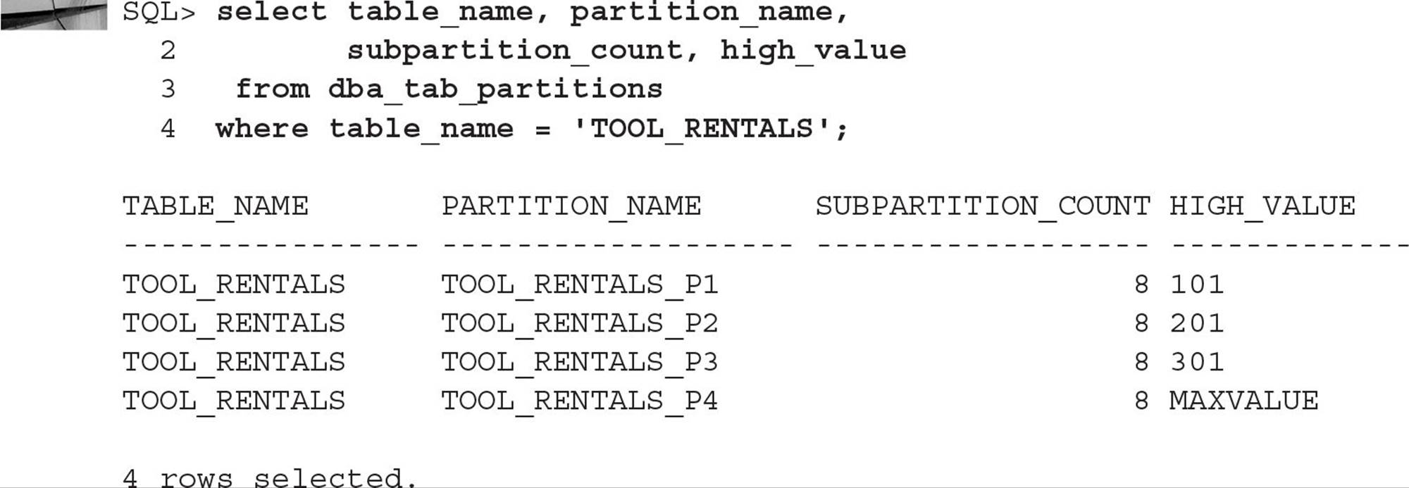
At the logical partition level, you still need to query DBA_TAB_PARTITIONS to obtain the range values, as you can see in the following query:

Also note that either the partition name or subpartition name can be specified to perform manual partition pruning, as in these two examples:

In the first query, a total of eight subpartitions are searched, TOOL_RENTALS_P1_S1 through TOOL_RENTALS_P1_S8; in the second query, only one out of the 32 total subpartitions is searched.

Using Composite Range-List Partitioning Similar to composite range-hash partitioning, composite range-list partitioning uses range partitioning to divide rows first using the range method and then subpartitioning the rows within each range using the list method. Composite range-list partitioning is good for historical data to place the data in each logical partition, further subdividing each logical partition using a discontinuous or discrete set of values.

NOTE

Range-list partitioning was introduced in Oracle 10g.

To use composite range-list partitioning, you must specify the following criteria:

Primary partitioning method (range)

Range partitioning column(s)

Partition names identifying the bounds of the partition

Subpartitioning method (list)

Subpartitioning column

Partition names, with each partition associated with a discrete list of literal values that place it in the partition

In the following example, we will expand on the previous “Sales by Region” list partitioning example and make the partitioned table more scalable by using the sales date for range partitioning, and we will use the state code for subpartitioning. Here is the CREATE TABLE command to accomplish this:

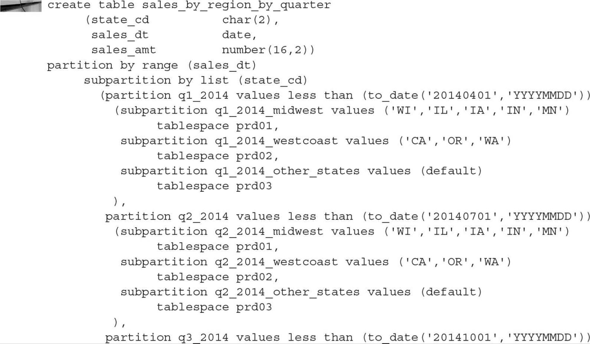
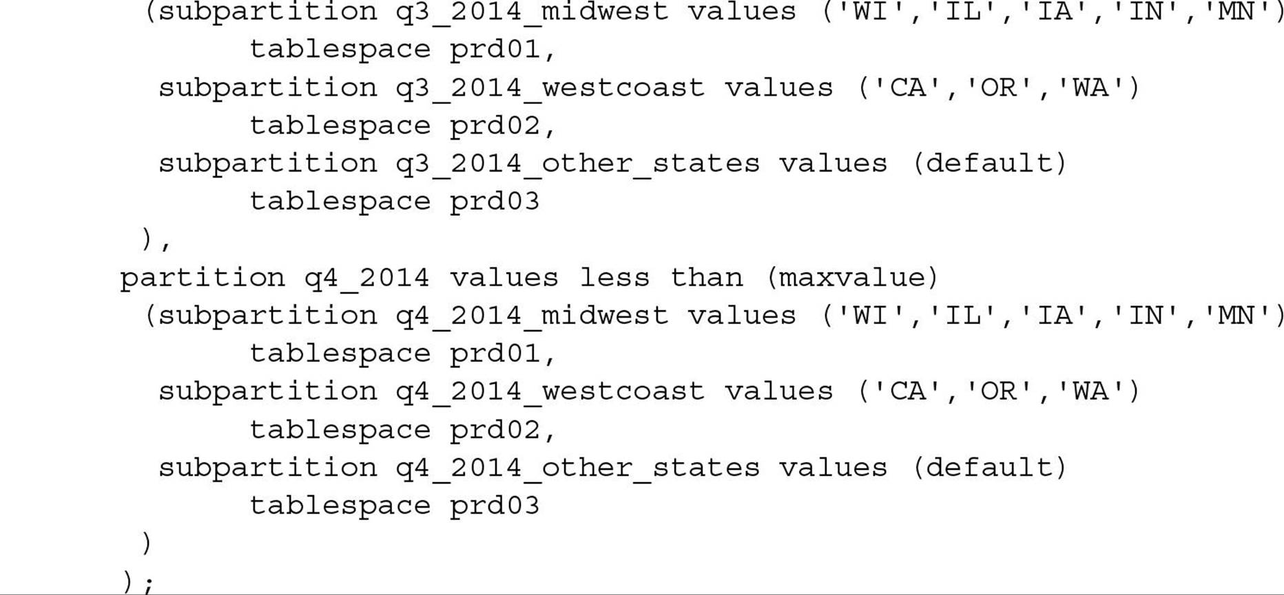
Each row stored in the table SALES_BY_REGION_BY_QUARTER is placed into one of 12 subpartitions, depending first on the sales date, which narrows the subpartition choice to three subpartitions. The value of the state code then determines which of the three subpartitions will be used to store the row. If a sales date falls beyond the end of 2014, it will still be placed in one of the subpartitions of Q4_2014 until you create a new partition and subpartitions for Q1_2015. Reorganizing partitioned tables is covered later in this chapter.

Using Composite List-Hash, List-List, and List-Range Partitioning Using list-hash, list-list, and list-range composite partitioning is similar to using range-hash, range-list, and range-range partitioning as discussed earlier in this section, except that you use the PARTITION BY LIST clause instead of the PARTITION BY RANGE clause as the primary partitioning strategy.

NOTE

Composite list-hash partitioning and all subsequent partitioning methods in this chapter are new as of Oracle 11g.

As an example, we’ll re-create the SALES_BY_REGION_BY_QUARTER table (which uses a range-list scheme) using a list-range partitioning scheme instead, as follows:

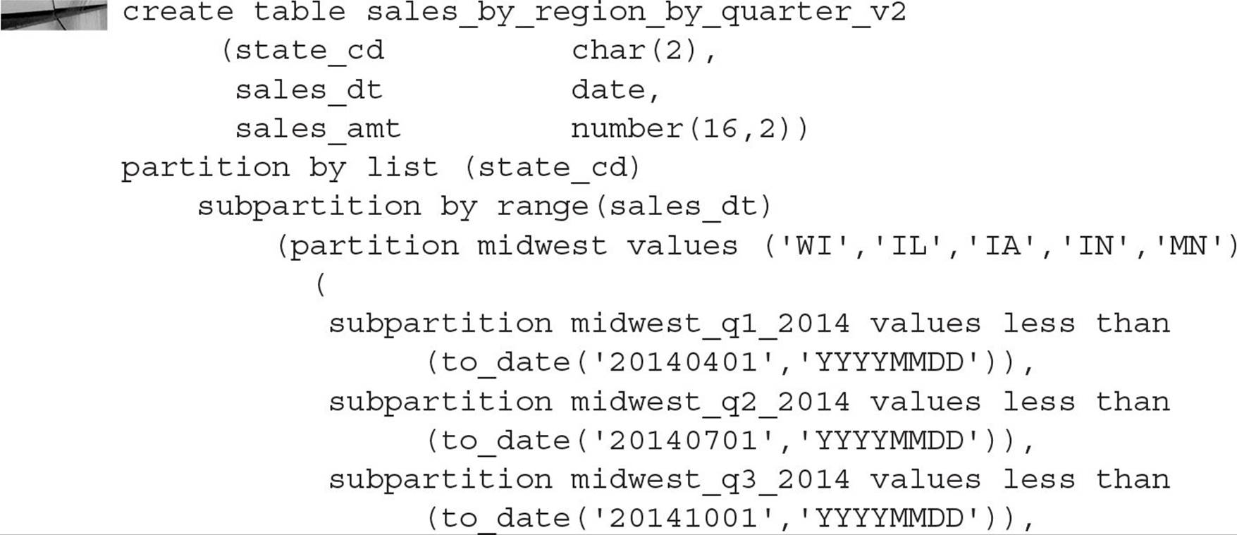
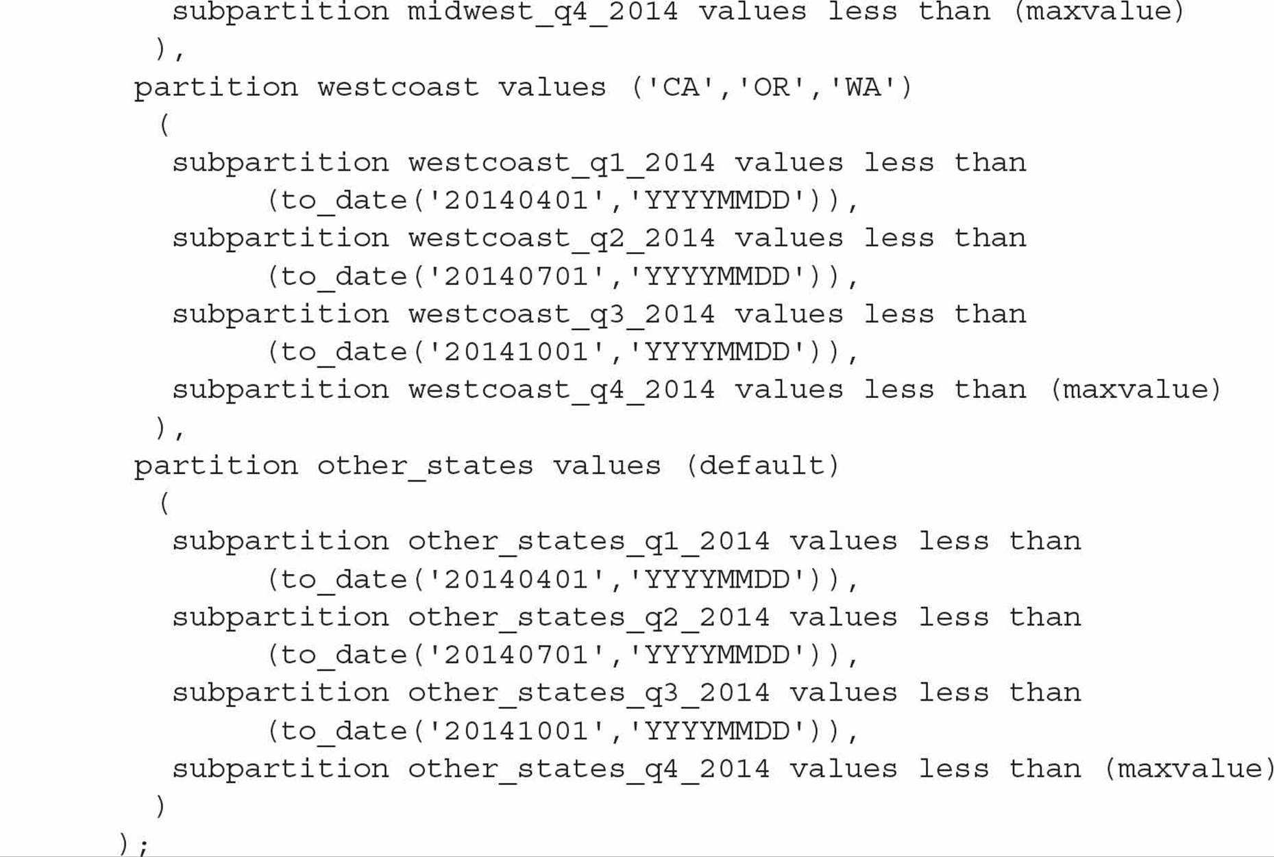
This alternate partitioning scheme makes sense if the regional managers perform their analyses by date only within their regions.

Using Composite Range-Range Partitioning As the name implies, the range-range partitioning method uses a range of values in two table columns. Both columns would otherwise lend themselves to a range-partitioned table, but the columns do not need to have the same datatype. For example, a medical analysis table can use a primary range column of patient birth date, and a secondary range column of patient birth weight in ounces. Here is an example of a patient table using these two attributes:

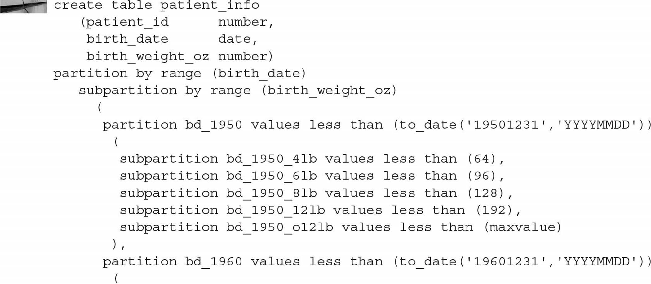
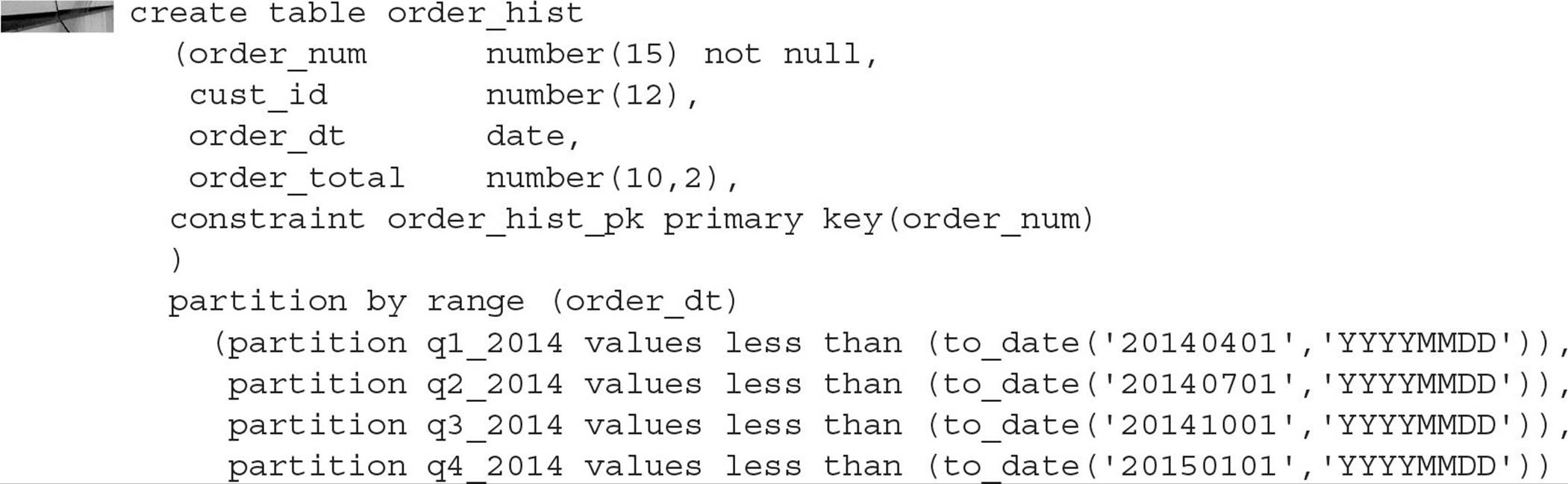
Using Interval Partitioning Interval partitioning automates the creation of new range partitions. For example, November, 2014 will almost certainly follow October, 2014, so using Oracle’s interval partitioning saves you the effort and creates and maintains new partitions when needed. Here is an example of a range-partitioned table with four partitions and an interval definition of one month:

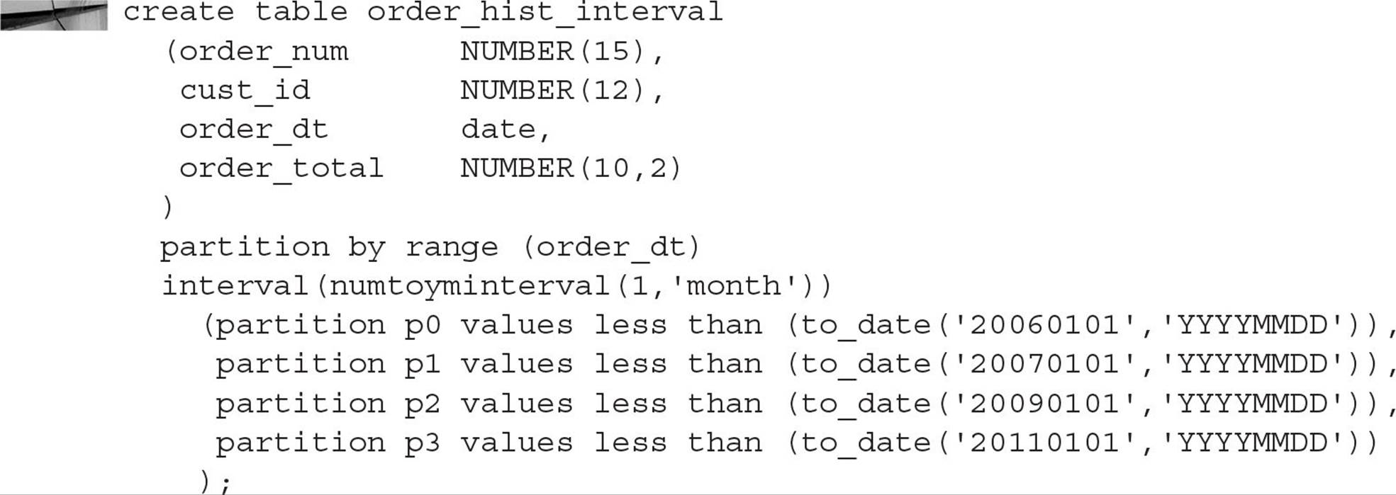
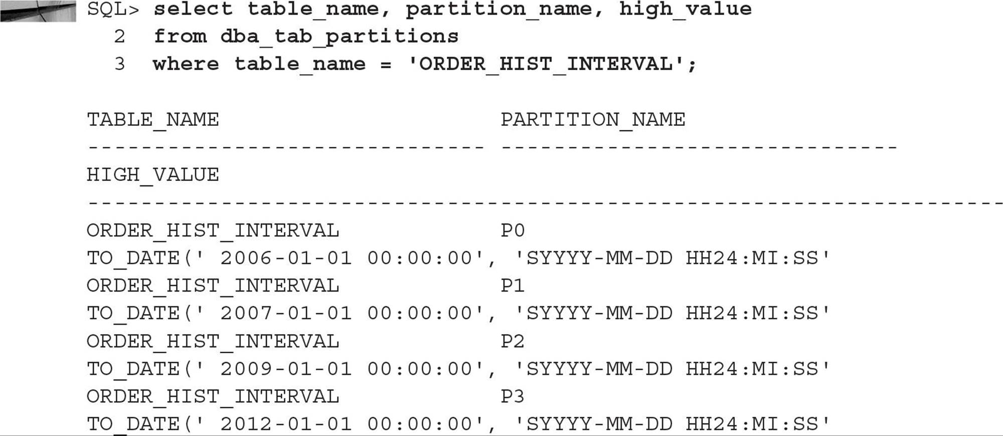
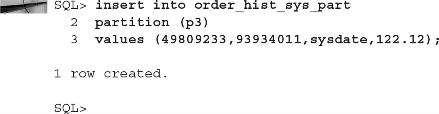
Rows inserted with an ORDER_DT of July 1, 2014, or earlier will reside in one of the four initial partitions of ORDER_HIST_INTERVAL. Rows inserted with an ORDER_DT after July 1, 2014, will trigger the creation of a new partition with a range of one month each; the upper bound of each new partition will always be the first of the month, based on the value of the highest partition’s upper limit. Looking in the data dictionary, this table looks somewhat like a pre-Oracle 11g range-partitioned table:

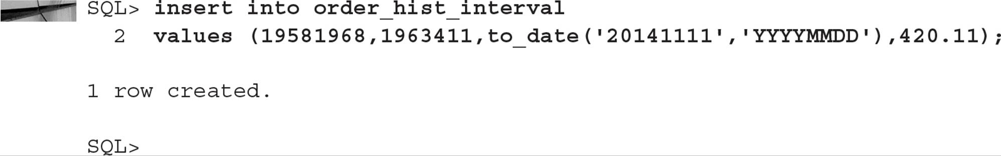
However, suppose you add a row for November 11, 2014, as in this example:

There is now a new partition, as you can see when you query DBA_TAB_PARTITIONS again:

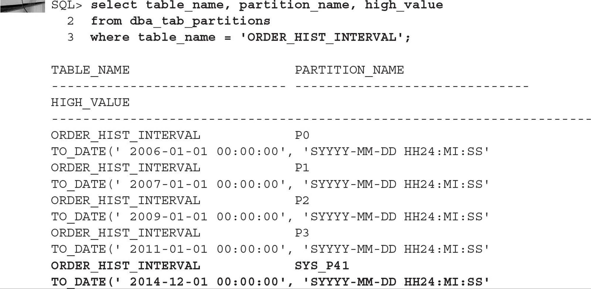
Note that partitions for July, August, September, and October of 2014 will not be created until order history rows are inserted containing dates within those months.

Using Reference Partitioning Reference partitioning leverages the parent-child relationships between tables to optimize partition characteristics and ease maintenance for tables that are frequently joined. In this example, the partitioning defined for the parent table ORDER_HIST is inherited by the ORDER_ITEM_HIST table:

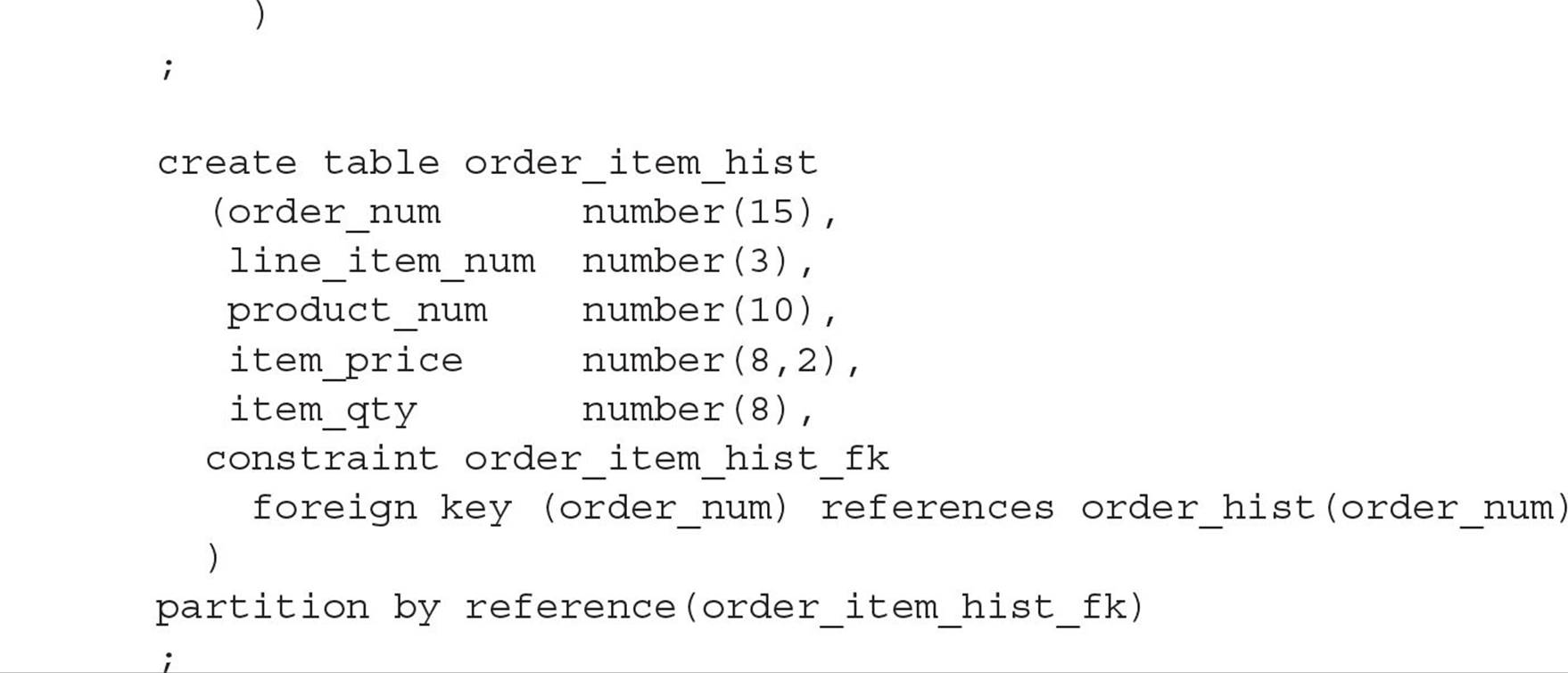
Oracle automatically creates corresponding partitions with the same name for the ORDER_ITEM_HIST as in ORDER_HIST.

Using Interval-Reference Partitioning As you might expect, interval-reference partitioning (new to Oracle Database 12c) combines the features of both interval partitioning and reference partitioning discussed in previous sections. The key difference is that the parent table is interval-partitioned instead of range-partitioned. This gives you yet another option to manage parent-child tables with automated interval partitioning. Here is the example from the previous section rewritten to use interval-reference partitioning:

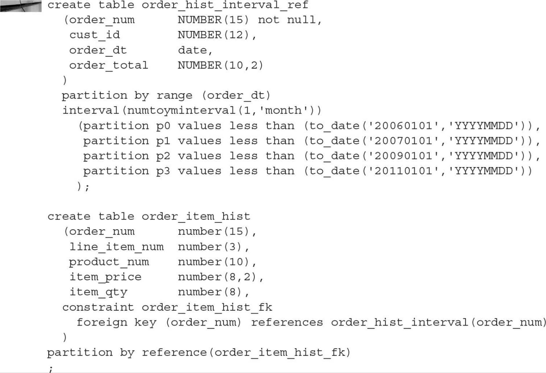
Any partition maintenance in the parent table (ORDER_HIST_INTERVAL) is automatically reflected in the child table (ORDER_ITEM_HIST). For example, converting a partition in the parent table from an interval partition to a conventional partition causes the same transformation in the child table.

Using Application-Controlled (System) Partitioning Application-controlled partitioning, also known as system partitioning, relies on the application logic to place rows into the appropriate partition. Only the partition names and the number of partitions are specified when the table is created, as in this example:

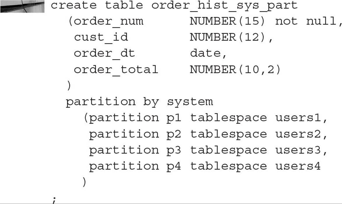
Any INSERT statements on this table must specify the partition number; otherwise, the INSERT will fail. Here is an example:

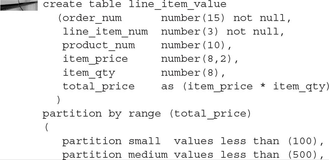
Using Virtual Column Partitioning Virtual columns, available starting in Oracle Database 11g, can also be used as a partition key; any partition method that uses a regular column can use a virtual column. In this example, you create a partitioned table for order items based on the total cost of the line item—in other words, number of items multiplied by the item price:

Using Compressed Partitioned Tables Partitioned tables can be compressed just as nonpartitioned tables can; in addition, the partitions of a partitioned table can be selectively compressed. For example, you may only want to compress the older, less often accessed partitions of a partitioned table and leave the most recent partition uncompressed to minimize the CPU overhead for retrieval of recent data. In this example, you will create a new version of the CAT_REQ table you created earlier in this chapter, compressing the first two partitions only. Here is the SQL command:

You do not have to specify NOCOMPRESS, because it is the default. To find out which partitions are compressed, you can use the column COMPRESSION in the data dictionary table DBA_TAB_PARTITIONS, as you can see in the following example:

Indexing Partitions

Local indexes on partitions reflect the structure of the underlying table and in general are easier to maintain than nonpartitioned or global partitioned indexes. Local indexes are equipartitioned with the underlying partitioned table; in other words, the local index is partitioned on the same columns as the underlying table and therefore has the same number of partitions and the same partition bounds as the underlying table.

Global partitioned indexes are created irrespective of the partitioning scheme of the underlying table and can be partitioned using range partitioning or hash partitioning. In this section, first I’ll show you how to create a local partitioned index; next, I’ll show you how to create both range-partitioned and hash-partitioned global indexes. In addition, I’ll show you how to save space in a partitioned index by using key compression.

Creating Local Partitioned Indexes A local partitioned index is very easy to set up and maintain because the partitioning scheme is identical to the partitioning scheme of the base table. In other words, the number of partitions in the index is the same as the number of partitions and subpartitions in the table; in addition, for a row in a given partition or subpartition, the index entry is always stored in the corresponding index’s partition or subpartition.

Figure 18-1 shows the relationship between a partitioned local index and a partitioned table. The number of partitions in the table is exactly the same as the number of partitions in the index.

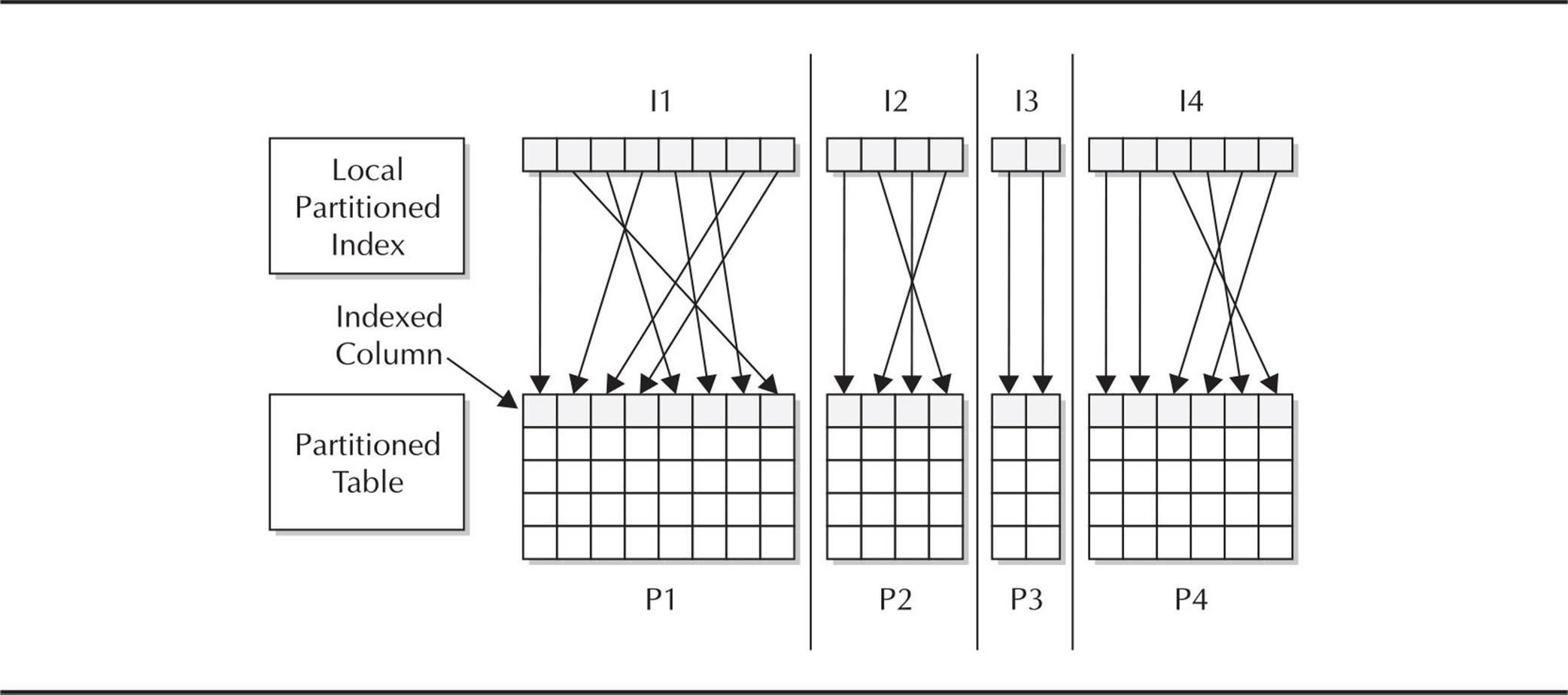
FIGURE 18-1. Local partitioned index on a partitioned table

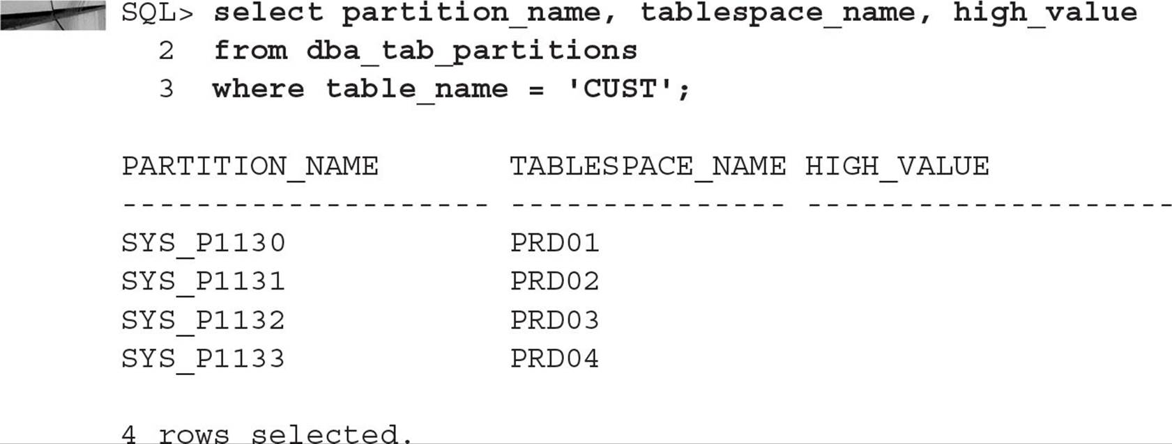
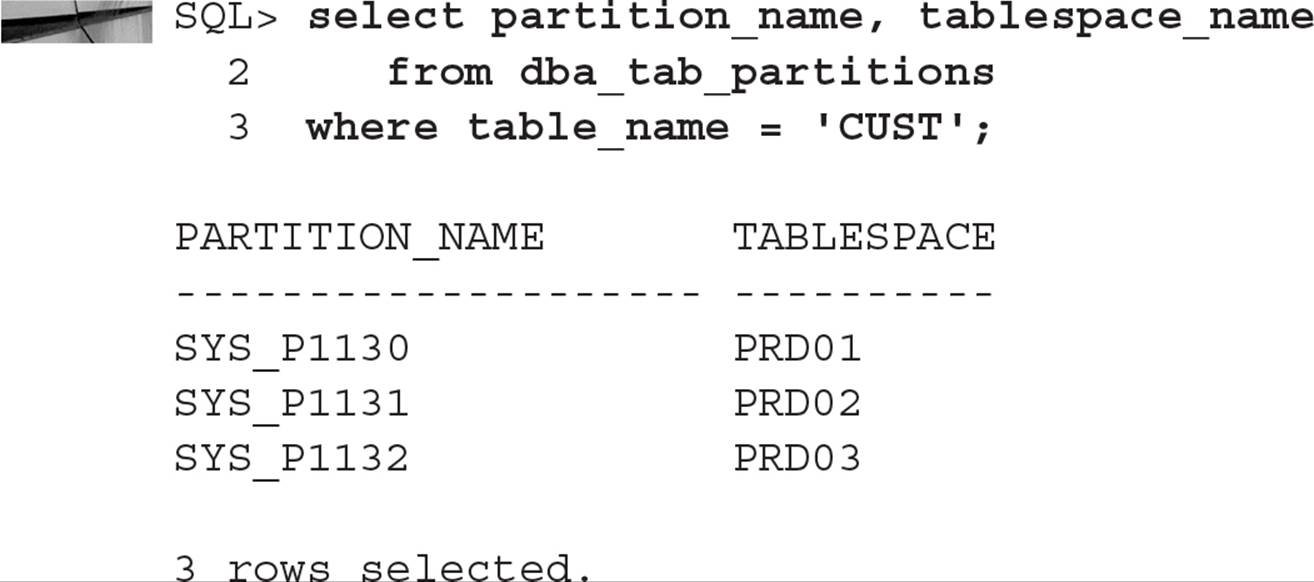
In the following example, you will create a local index on the CUST table you created earlier in the chapter. Here is the SQL statement that retrieves the table partitions for the CUST table:

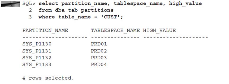
The command for creating the local index on this table is very straightforward, as you can see in this example:

The index partitions are stored in four tablespaces stored outside of an ASM disk group—IDX_1 through IDX_4—to further improve the performance of the table, because each index partition is stored in a tablespace separate from any of the table partitions. You can find out about the partitions for this index by querying DBA_IND_PARTITIONS, as follows:

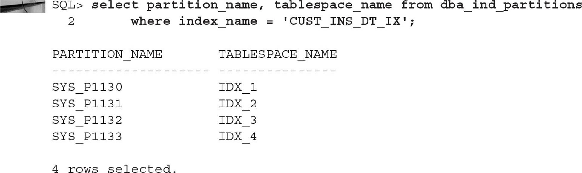
Notice that the index partitions are automatically named the same as their corresponding table partitions. One of the benefits of local indexes is that when you create a new table partition, the corresponding index partition is built automatically; similarly, dropping a table partition automatically drops the index partition without invalidating any other index partitions, as would be the case for a global index.

Creating Range-Partitioned Global Indexes Creating a range-partitioned global index involves rules similar to those you use when creating range-partitioned tables. In a previous example, you created a range-partitioned table called CAT_REQ that contained four partitions based on the CAT_REQ_DT column. In this example, you will create a partitioned global index that will only contain two partitions (in other words, not partitioned the same way as the corresponding table):

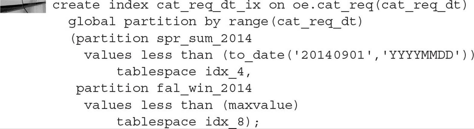
Note that you specify two tablespaces to store the partitions for the index that are different from the tablespaces used to store the table partitions. If any DDL activity occurs on the underlying table, global indexes are marked as UNUSABLE and need to be rebuilt unless you include the UPDATE GLOBAL INDEXES clause (INVALIDATE GLOBAL INDEXES is the default). In the section “Managing Partitions” later in this chapter, we will review the UPDATE INDEX clause when you are performing partition maintenance operations on partitioned indexes.

Figure 18-2 shows the relationship between a partitioned global index and a partitioned table. The number of partitions in the table may or may not be the same as the number of partitions in the index.

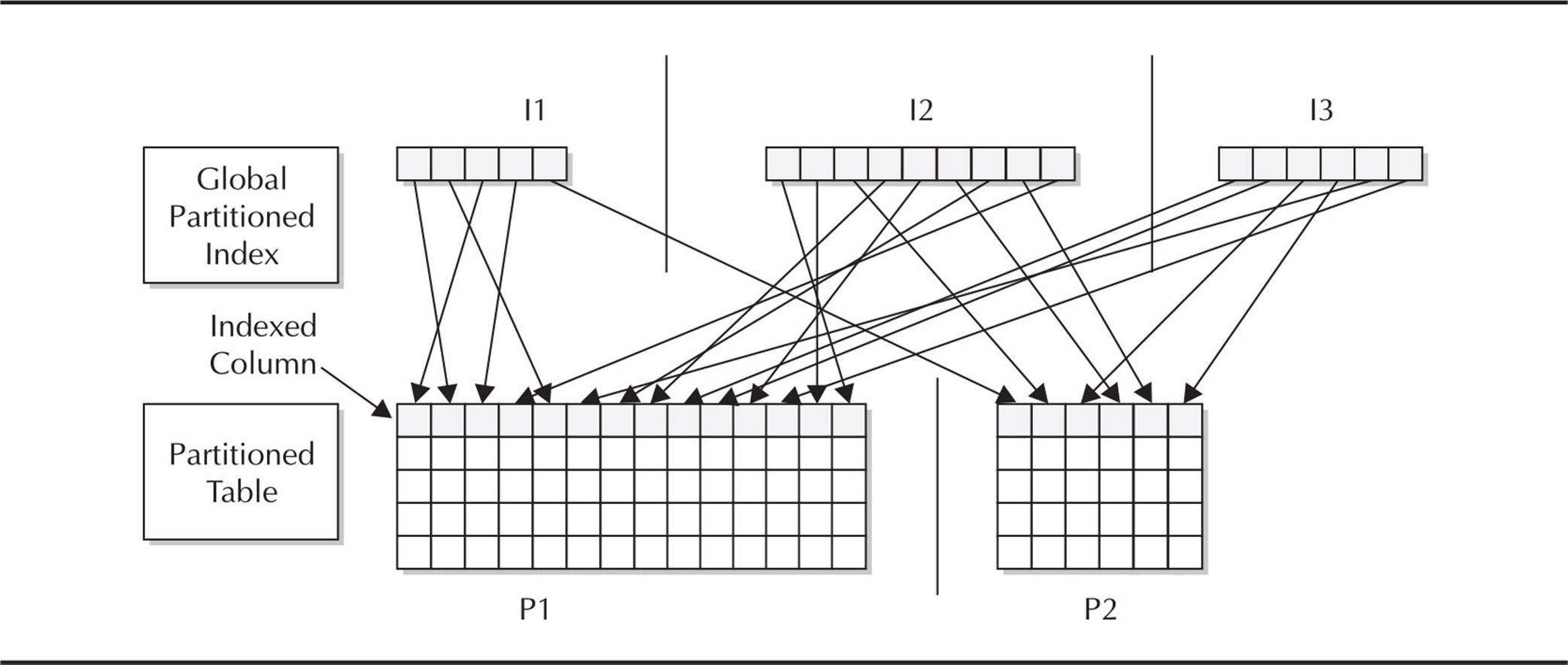
FIGURE 18-2. Global partitioned index on a partitioned table

Creating Hash-Partitioned Global Indexes As with range-partitioned global indexes, hash-partitioned global index CREATE statements share the syntax with hash-partitioned table CREATE statements. Hash-partitioned global indexes can improve performance in situations where a small number of a nonpartitioned index’s leaf blocks are experiencing high contention in an OLTP environment. Queries that use either an equality or IN operator in the WHERE clause can benefit significantly from a hash-partitioned global index.

NOTE

Hash-partitioned global indexes are new as of Oracle 10g.

Building on our example using hash partitioning for the table CUST, you can create a hash-partitioned global index on the ZIP_CD column:

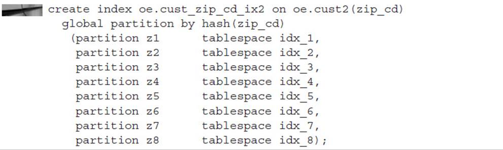
Note that the table CUST2 is partitioned using the CUST_NUM column, and it places its four partitions in PRD01 through PRD04; this index partition uses the ZIP_CD column for the hashing function and stores its eight partitions in IDX_1 through IDX_8.

Creating Nonpartitioned Global Indexes Creating a nonpartitioned global index is the same as creating a regular index on a nonpartitioned table; the syntax is identical. Figure 18-3 shows the relationship between a nonpartitioned global index and a partitioned table.

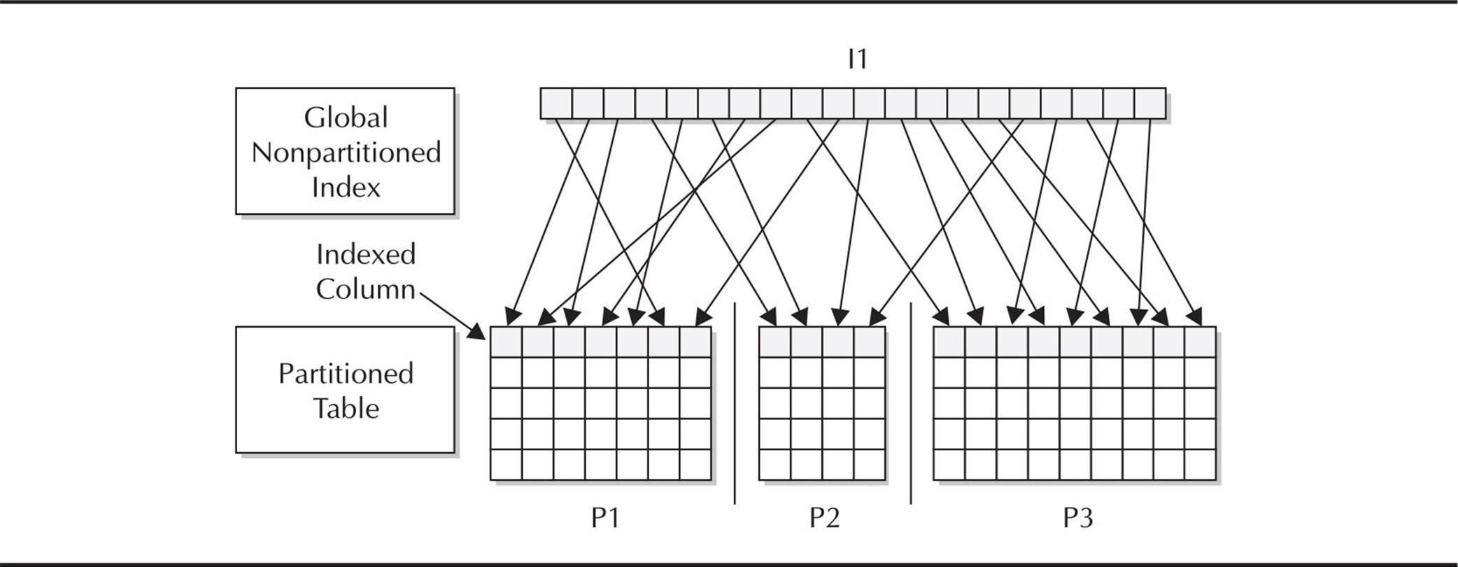
FIGURE 18-3. Global nonpartitioned index on a partitioned table

Using Key Compression on Partitioned Indexes If your index is nonunique and has a large number of repeating values for the index key or keys, you can use key compression on the index just as you can with a traditional nonpartitioned index. When only the first instance of the index key is stored, both disk space and I/O are reduced. In the following example, you can see how easy it is to create a compressed partitioned index:

You can specify that a more active index partition not be compressed by using NOCOMPRESS, which may save a noticeable amount of CPU for recent index entries that are more frequently accessed than the others in the index.

Partitioned Index-Organized Tables

Index-organized tables (IOTs) can be partitioned using either the range, list, or hash partitioning method; creating partitioned index-organized tables is syntactically similar to creating partitioned heap-organized tables. In this section, we’ll cover some of the notable differences in how partitioned IOTs are created and used.

For a partitioned IOT, the ORGANIZATION INDEX, INCLUDING, and OVERFLOW clauses are used as they are for standard IOTs. In the PARTITION clause, you can specify the OVERFLOW clause as well as any other attributes of the overflow segment specific to a partition.

Since Oracle Database 10g, there is no longer the restriction that the set of partitioning columns must be a subset of the IOT’s primary key columns; in addition, LIST partitioning is supported in addition to range and hash partitioning. In previous releases of Oracle, LOB columns were supported only in range-partitioned IOTs; as of Oracle 10g, they are supported in hash and list partitioning methods as well.

Managing Partitions

Fourteen maintenance operations can be performed on a partitioned table, including splitting a partition, merging partitions, and adding a new partition. These operations may or may not be available depending on the partitioning scheme used (range, hash, list, or one of the six composite methods). For composite partitions, these operations sometimes apply to both the partition and the subpartition, and sometimes to the subpartition only.

For partitioned indexes, there are seven different types of maintenance operations that vary depending on both the partitioning method (range, hash, list, or composite) as well as whether the index is a global index or a local index. In addition, each type of partitioned index may support automatic updates when the partitioning scheme is changed, thus reducing the occurrences of unusable indexes.

In the next couple sections, I’ll present a convenient chart for both partitioned tables and partitioned indexes that shows you what kinds of operations are allowed on which partition types. For some of the more common maintenance operations, I’ll give you some examples of how they are used, extending some of the examples I have presented earlier in this chapter.

Maintaining Table Partitions To maintain one or more table partitions or subpartitions, you use the ALTER TABLE command just as you would on a nonpartitioned table. In Table 18-5 are the types of partitioned table operations and the keywords you would use to perform them. The format of the ALTER TABLE command is as follows:

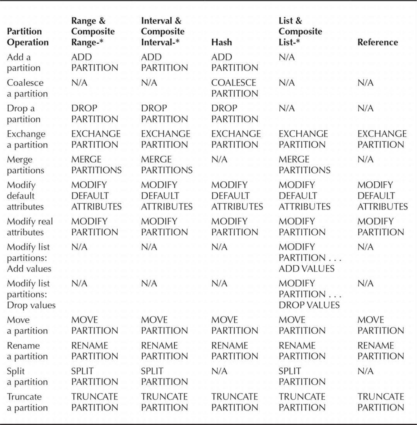
TABLE 18-5. Maintenance Operations for Partitioned Tables

Table 18-6 contains the subpartition table operations.

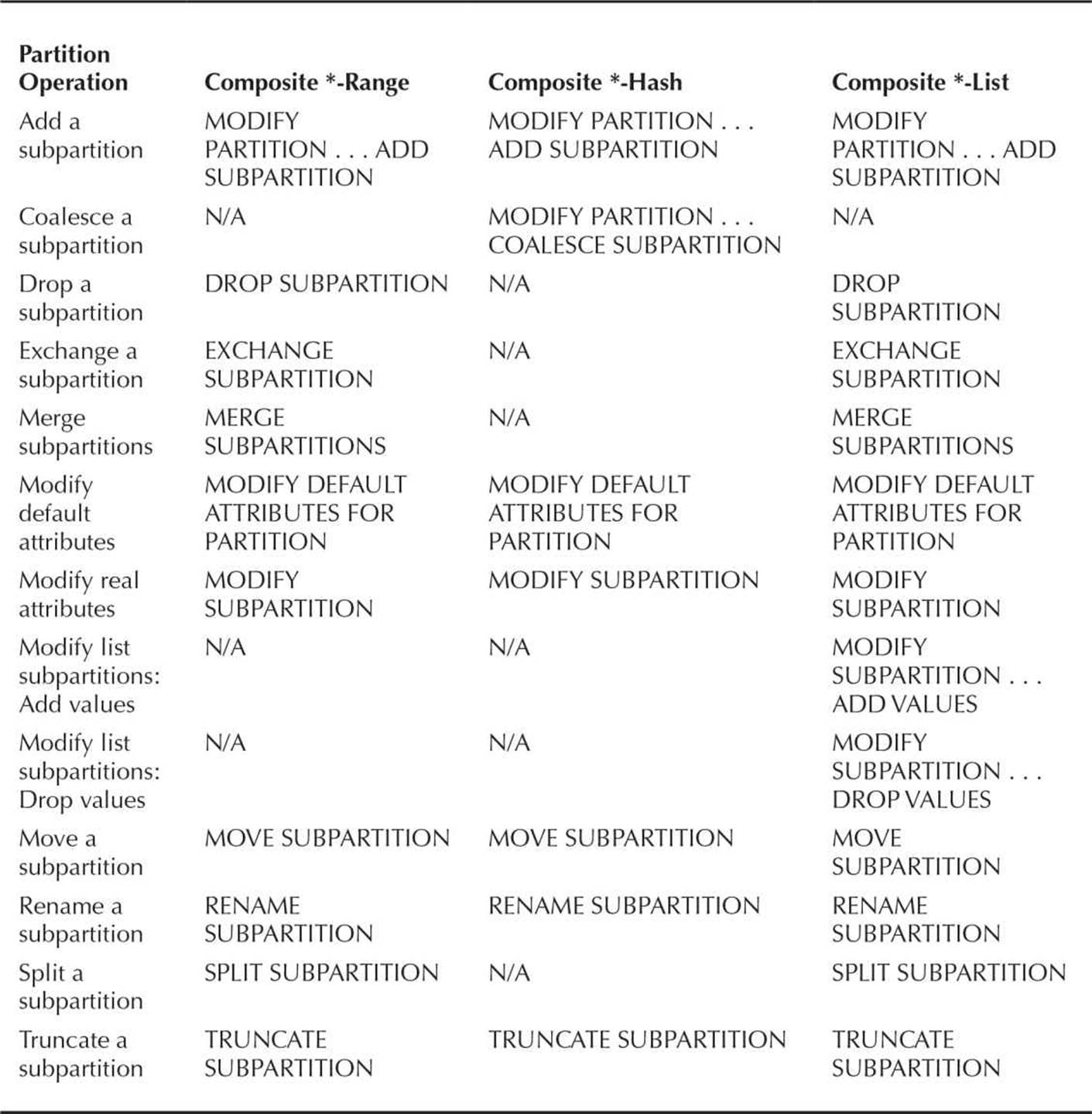
TABLE 18-6. Maintenance Operations for Subpartitions of Partitioned Tables

CAUTION

Using the ADD PARTITION clause only works if there are no existing entries for new partitions in the DEFAULT partition.

In many cases, partitioned table maintenance operations invalidate the underlying index; while you can always rebuild the index manually, you can specify UPDATE INDEXES in the table partition maintenance command. Although the table maintenance operation will take longer, the most significant benefit of using UPDATE INDEXES is to keep the index available during the partition maintenance operation.

Splitting, Adding, and Dropping Partitions In many environments, a “rolling window” partitioned table will contain the latest four quarters’ worth of rows. When the new quarter starts, a new partition is created, and the oldest partition is archived and dropped. In the following example, you will split the last partition of the CAT_REQ table you created earlier in this chapter at a specific date and maintain the new partition with MAXVALUE, back up the oldest partition, and then drop the oldest partition. Here are the commands you can use:

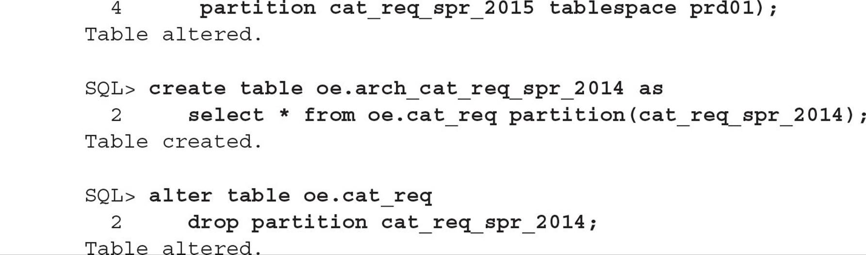
The data dictionary view DBA_TAB_PARTITIONS reflects the new partitioning scheme, as you can see in this example:

Note that if you had dropped any partition other than the oldest partition, the next highest partition “takes up the slack” and contains any new rows that would have resided in the dropped partition; regardless of what partition is dropped, the rows in the partition are no longer in the partitioned table. To preserve the rows, you would use MERGE PARTITION instead of DROP PARTITION.

Coalescing a Table Partition You can coalesce a partition in a hash-partitioned table to redistribute the contents of the partition to the remaining partitions and reduce the number of partitions by one. For the new CUST table you created earlier in this chapter, you can do this in one easy step:

The number of partitions in CUST is now three instead of four:

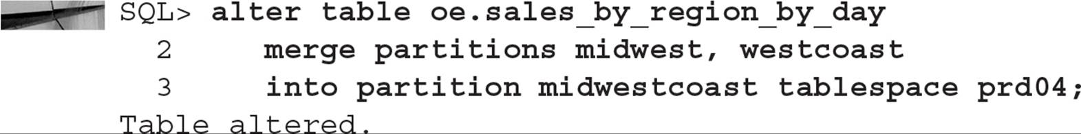
Merging Two Table Partitions You may find out through various Oracle advisors that one partition of a partitioned table is infrequently used or not used at all; in this situation, you may want to combine two partitions into a single partition to reduce your maintenance effort. In this example, you will combine the partitions MIDWEST and WESTCOAST in the partitioned table SALES_BY_REGION_BY_DAY into a single partition, MIDWESTCOAST:

Looking at the data dictionary view DBA_TAB_PARTITIONS, you can see that the table now has only two partitions:

Maintaining Index Partitions To maintain one or more index partitions or subpartitions, you use the ALTER INDEX command just as you would on a nonpartitioned index. Table 18-7 lists the types of partitioned index operations and the keywords you would use to perform them for the different types of partitioned indexes (range, hash, list, and composite). The format of the ALTER INDEX command is

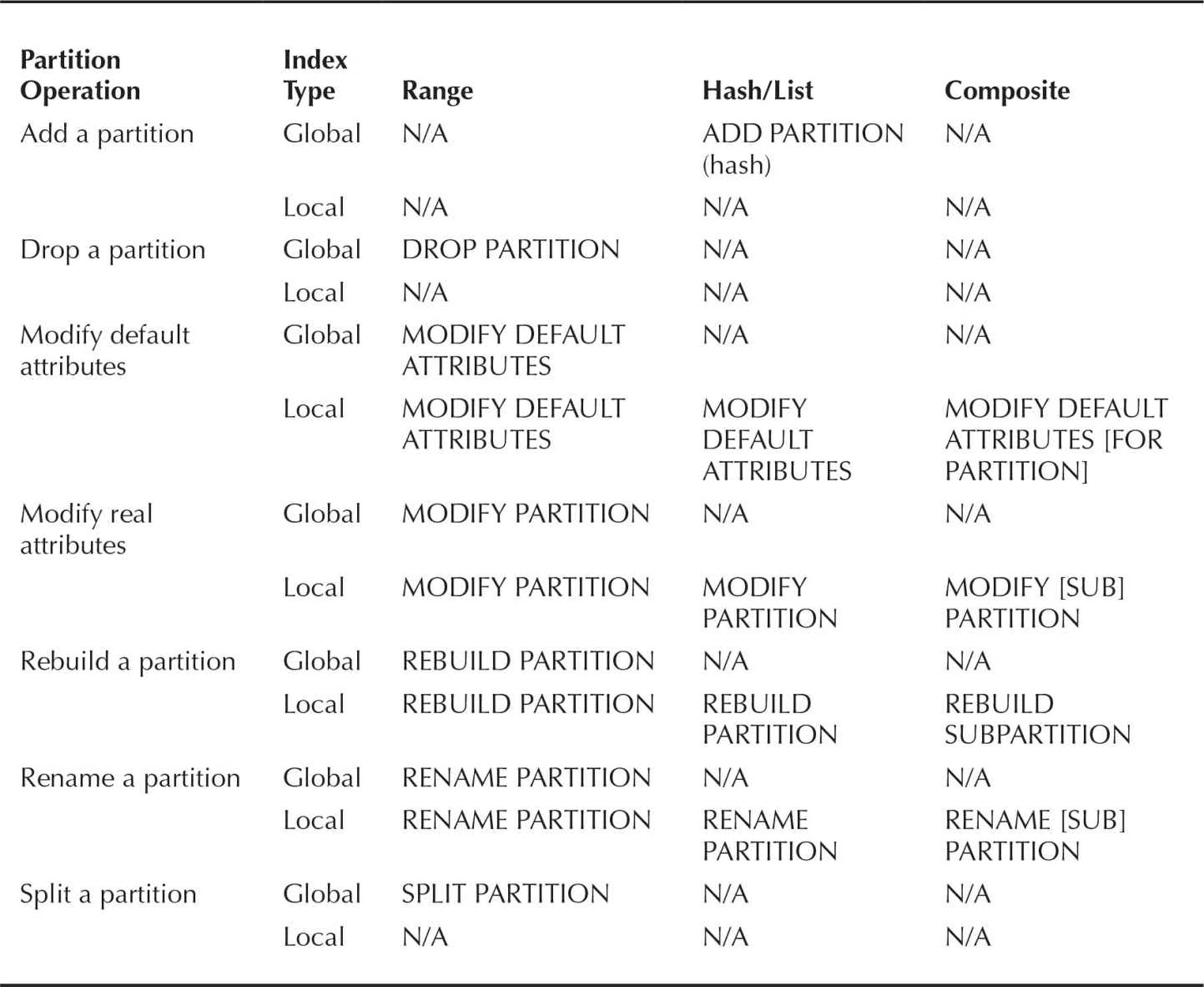
TABLE 18-7. Maintenance Operations for Partitioned Indexes

As with table partition maintenance commands, not all operations are available for every index partition type. You should note that many of the index partition maintenance options do not apply to local index partitions. By its nature, a local index partition matches the partitioning scheme of the table and will change when you modify the table’s partitioning scheme.

Splitting a Global Index Partition Splitting a global index partition is much like splitting a table’s partition. One particular global index partition may be a hotspot due to the index entries being stored in that particular partition; as with a table partition, you can split the index partition into two or more partitions. In the following example, you’ll split one of the partitions of the global index OE.CAT_REQ_DT_IX into two partitions:

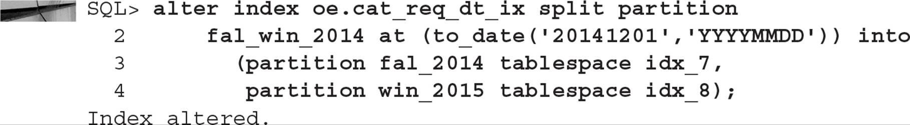
The index entries for the FAL_WIN_2014 partition will now reside in two new partitions, FAL_2014 and WIN_2015.

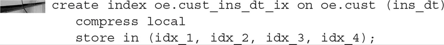
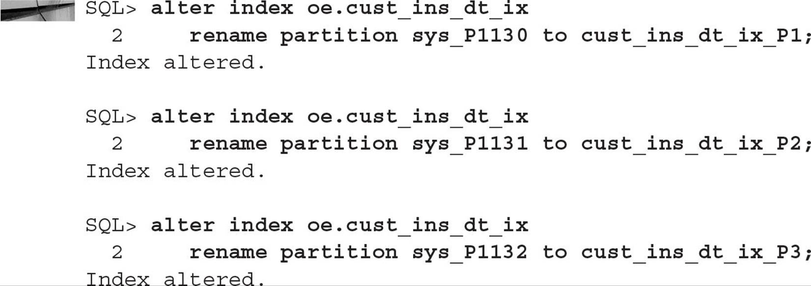
Renaming a Local Index Partition Most characteristics of a local index are updated automatically when the corresponding table partition is modified. However, a few operations still may need to be performed on a local index partition, such as rebuilding the partition or renaming a partition that was originally named with a default system-assigned name. In this example, you will rename the local index partitions in the index OE.CUST_INS_DT_IX using more meaningful names:

Materialized Views

Another type of table, called a materialized view, shares the characteristics of a table and a view. It is like a view in that it derives its results from a query against one or more tables; it is like a table in that it persists the result set of a view in a segment. Materialized views are useful in both OLTP and DSS systems. Frequent user queries against operational data may be able to use materialized views instead of the repeated joining of many highly normalized tables, and in a data warehouse environment the historical data can be aggregated ahead of time to make DSS queries run in a fraction of the time it would take to aggregate the data “on the fly.”

The data in a materialized view can be refreshed on demand or incrementally, depending on the business need. Depending on the complexity of the view’s underlying SQL statement, the materialized view can be quickly brought up to date with incremental changes via a materialized view log.

To create a materialized view, you use the CREATE MATERIALIZED VIEW command; the syntax for this command is similar to creating a standard view. Because a materialized view stores the result of a query, you can also specify storage parameters for the view as if you were creating a table. In the CREATE MATERIALIZED VIEW command, you also specify how the view will be refreshed. The materialized view can be refreshed either on demand or whenever one of the base tables changes. Also, you can force a materialized view to use materialized view logs for an incremental update, or you can force a complete rebuild of the materialized view when a refresh occurs.

Materialized views can automatically be used by the optimizer if the optimizer determines that a particular materialized view already has the results of a query that a user has submitted; the user does not even have to know that their query is using the materialized view directly instead of the base tables. However, to use query rewrite, the user must have the QUERY REWRITE system privilege and you have to set the value of the initialization parameter QUERY_REWRITE_ENABLED to TRUE.

Using Bitmap Indexes

An alternative to B-tree indexes, called bitmap indexes, provides query optimization benefits in environments that frequently perform joins on columns with low cardinality. In this section, we’ll review the basics of bitmap indexes, create a bitmap index, and look at how bitmap indexes can be created ahead of time against columns in two or more tables.

Understanding Bitmap Indexes

A bitmap index is extremely useful in a VLDB environment when the column being indexed has a very low number of possible values, such as gender, where the possible values are usually M and F. A bitmap index uses a string of binary ones and zeros to represent the existence or nonexistence of a particular column value. Using bitmap indexes makes multiple AND and OR operations against several table columns very efficient in a query. Bitmap indexes are common in data warehouse and other VLDB environments where many low-cardinality columns exist, DML commands are done in bulk, and the query conditions frequently use columns with bitmap indexes.

The space requirements for a bitmap index are low as long as the cardinality is low; for example, a bitmap index on the GENDER column of the EMPLOYEES table would contain two bitmaps with a length equal to the number of rows in the table. If the EMPLOYEES table had 15 rows, the bitmaps for the GENDER column might look like the following:

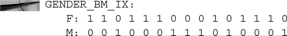
As you can see, the size of the bitmap index is directly proportional to the cardinality of the column being indexed; however, bitmap index blocks with all zeros are compressed to reduce storage space for bitmap indexes. A bitmap index on the LAST_NAME column of the EMPLOYEES table would be significantly larger, and many of the benefits of a bitmap index in this case might be outweighed by the space consumed by the index! Although there are exceptions to every rule, the cardinality can be up to ten percent of the rows and bitmap indexes will still perform well; in other words, a table with 1000 rows and 100 distinct values in a particular column will still most likely benefit from a bitmap index.

NOTE

The Oracle optimizer dynamically converts bitmap index entries to ROWIDs during query processing. This allows the optimizer to use bitmap indexes with B-tree indexes on columns that have many distinct values.

Previous to Oracle 10g, the performance of a bitmap would often deteriorate over time with frequent DML activity against the table containing the bitmap index. To take advantage of the improvements to the internal structure of bitmap indexes, you must set the COMPATIBLE initialization parameter to 10.0.0.0 or greater (to match your current release: if you’re using Oracle Database 12c, you should have COMPATIBLE set to 12.1.0 or higher). Bitmap indexes that performed poorly before the COMPATIBLE parameter was adjusted should be rebuilt; bitmap indexes that performed adequately before the COMPATIBLE parameter was changed will perform better after the change. Any new bitmap indexes created after the COMPATIBLE parameter is adjusted will take advantage of all improvements.

Using Bitmap Indexes

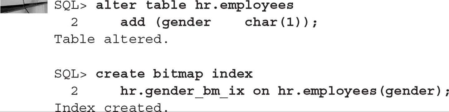
Bitmap indexes are easy to create; the syntax is identical to that for creating any other index, with the addition of the BITMAP keyword. In the following example, you will add a GENDER column to the EMPLOYEES table and then create a bitmap index on it:

Using Bitmap Join Indexes

As of Oracle9i, you can create an enhanced type of bitmap index called a bitmap join index. A bitmap join index is a bitmap index representing the join between two or more tables. For each value of a column in the first table of the join, the bitmap join index stores the ROWIDs of the corresponding rows in the other tables with the same value as the column in the first table. Bitmap join indexes are an alternative to materialized views that contain a join condition; the storage required for storing the related ROWIDs can be significantly lower than storing the result of the view itself.

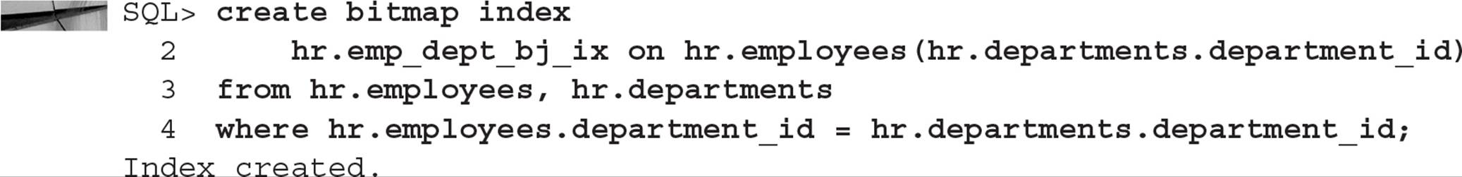
In this example, you find out that the HR department is frequently joining the EMPLOYEES and DEPARTMENTS table on the DEPARTMENT_ID column. As an alternative to creating a materialized view, you decide to create a bitmap join index. Here is the SQL command to create the bitmap join index:

There are a few restrictions on bitmap join indexes:

Only one of the tables in the bitmap join index can be updated concurrently by different transactions when the bitmap join index is being used.

No table can appear more than once in the join.

Bitmap join indexes cannot be created on an IOT or a temporary table.

A bitmap join index cannot be created with the UNIQUE attribute.

The join column(s) used for the index must be the primary key or have a unique constraint in the table being joined to the table with the bitmap index.

Summary

Chances are your database gets bigger rather than smaller every day. More customers are buying your merchandise online, for example, or more patients are being seen by doctors in your health system every day, and all of this information either should or must be retained over time for analytical or legal reasons. Therefore, Oracle Database 12c makes it easy to manage and access both current and historical data.

Bigfile tablespaces break past the limitations in datafile size for a tablespace (32GB for an 8KB block size, for example). Not only does this reduce the number of datafiles you need in your database but also enables maintenance of the tablespace at the tablespace level instead of the datafile level.

Table and index partitioning is the key feature of Oracle Database 12c (and the previous few versions!) that enables the timely access of rows from tables with millions or billions of rows. Even with an indexed table you may have to traverse billions of index entries to find the rows you need when all you need are the last three months’ worth of rows in a patient visit table. Using an encounter date as the partitioning key means that even a full table scan on the last three months’ worth of patient visits (the latest three partitions) will take seconds instead of hours.

Finally, bitmap indexes can speed up a class of queries where you typically have a low number of values in a column and you want to quickly filter a large percentage of those rows by using a very compact bitmap index whose format is literally a single bit for the existence of that column’s value in the current row of the table. Bitmap join indexes take it a step further by pre-joining a column that’s common to two tables, further speeding up any future joins between those two tables.