Learning Informatica PowerCenter 9.x (2014)

Chapter 7. The Lifeline of Informatica – Transformations

Transformations are the most important aspect of the Informatica PowerCenter tool. The functionality of any ETL tool lies in transformations. Needless to say, transformations are used to transform data. Informatica PowerCenter provides multiple transformations, each serving a particular functionality. Transformations can be created as reusable or nonreusable based on the requirement. The transformations created in Workflow Manager are nonreusable, and those created in the task developer are reusable. You can create a mapping with a single transformation or with multiple transformations.

When you run the workflow, Integration Services extracts the data in a row-wise manner from the source path/connection you defined in the session task and makes it flow from the mapping. The data reaches the target through the transformations you defined.

The data always flows in a row-wise manner in Informatica no matter what your calculation or manipulation is. So if you have 10 records in source, there will be 10 source to target flows while the process is executed.

Creating the transformation

There are various ways in which you can create the transformation in the Designer tool. They are discussed in the upcoming sections.

Mapping Designer

To create transformations using Mapping Designer, perform the following steps:

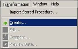
1. Open the mapping in Mapping Designer. Then open the mapping in which you wish to add a transformation, and navigate to Transformation | Create.

2. From the drop-down list of transformations, select the transformation you wish to create, and specify the name. Click on Create, and then click on Done.

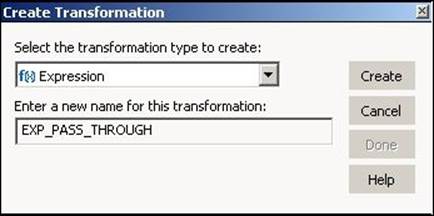
The transformation appears in the Mapping Designer Workspace. For reference, we have created an Expression transformation in the preceding image. You can create all other transformations in the same way.

The transformations you create in Mapping Designer are nonreusable, so you cannot use them in other mappings. However, you can change the transformation to reusable.

Mapplet Designer

To create the transformation in Mapplet Designer, perform the following steps:

1. Open the Mapplet in Mapplet Designer, and navigate to Transformation | Create, as shown in the preceding screenshot.

2. From the drop-down list of transformations, select the transformation you wish to create and specify the name.

Transformation Developer

To create the transformation in the designer, perform the following steps:

1. Open Transformation Developer and navigate to Transformation | Create as shown in Mapping Designer.

2. From the drop-down list of transformations, select the transformation you wish to create and specify the name as shown in Mapping Designer.

The transformations created in Transformation Developer are reusable, so you can use them across multiple mappings or mapplets.

With this basic understanding, we are all set to jump into the most important aspect of the Informatica PowerCenter tool, which is transformation.

The Expression transformation

Expression transformations are used for row-wise manipulation. For any type of manipulation you wish to perform on an individual record, use an Expression transformation. The Expression transformation accepts the row-wise data, manipulates it, and passes it to the target. The transformation receives the data from the input port and sends the data out from output ports.

Use Expression transformations for any row-wise calculation, such as if you want to concatenate the names, get the total salary, and convert it to uppercase. To understand the functionality of the Expression transformation, let's take a scenario.

Using flat file as the source, which we we created in Chapter 1, Starting the Development Phase – Using the Designer Screen Basics, concatenate FIRST_NAME and LAST_NAME to get FULL_NAME and TOTAL_SALARY from JAN_SALARY and FEB_SALARY of an individual employee.

We are using Expression transformation in this scenario because the value of FULL_NAME can be achieved by concatenating FIRST_NAME and LAST_NAME of an individual record. Similarly, we can get TOTAL_SALARY using JAN_SALARY and FEB_SALARY. In other words, the manipulation required is row-wise.

We are going to learn some basic aspects of transformations, such as ports in transformations, writing a function, and so on while we implement our first transformation using an expression.

Perform the following steps to achieve the functionality:

1. Create the source using flat file in Source Analyzer and the target in Target Designer. We will be using EMP_FILE as the source and TGT_EMP_FILE as the target.

2. Create a new m_EXP_CONCAT_TOTAL mapping in Mapping Designer, drag the source and target from the navigator to the workspace, and create the Expression transformation with the EXP_CONCAT_TOTAL name.

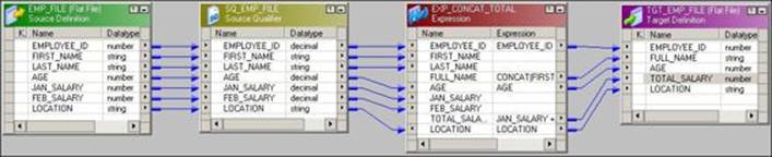
3. Drag-and-drop all the columns from the source qualifier to the Expression transformation. At this point, the mapping will look as shown in the following screenshot:

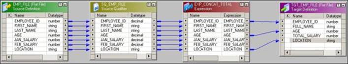
We have connected EMPLOYEE_ID, AGE, and LOCATION directly to the target as no manipulation is required for these columns.

At this step, we need to understand how to use the different types of ports in the transformation.

Ports in transformations

Transformations receive the data from input ports and send the data out using output ports. Variable ports temporarily store the value while processing the data.

Every transformation, with a few exceptions, has input and output ports as shown in the following screenshot:

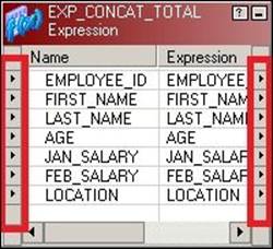
Double-click on the transformation and click on Ports to open the edit view and see the input, output, and variable ports.

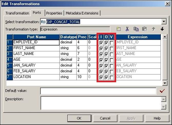
You can disable or enable input or output ports based on the requirement. In our scenario, we need to use the values that come from input ports and send them using an output port using concatenate, by writing the function in the expression editor.

Create two new output ports for FULL_NAME after LAST_NAME and TOTAL_SALARY after FEB_SALARY. We need to add the FULL_NAME port after LAST_NAME, because the FULL_NAME port will use the values in FIRST_NAME and LAST_NAME. To add a new port, double-click on the Expression transformation, click on Ports, and add two new output ports, as shown in the following screenshot:

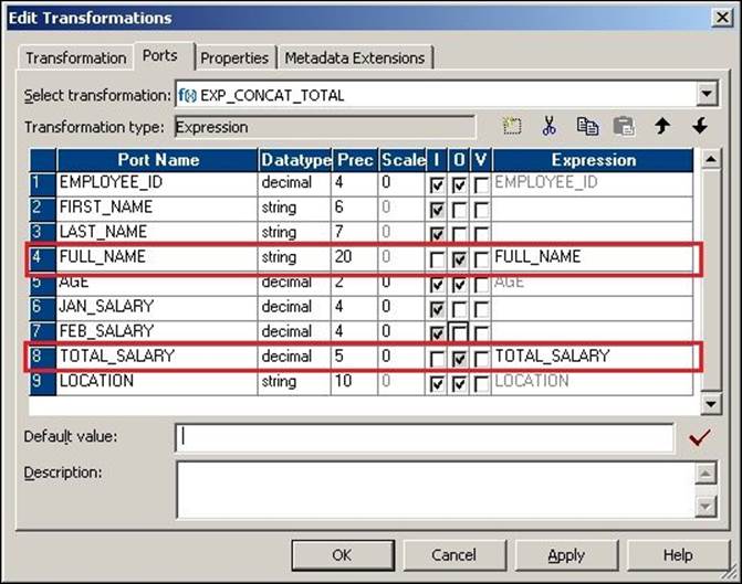
Make sure you define the proper data type and size of the new ports that are added. As you can see, we have disabled the input ports of FULL_NAME and TOTAL_SALARY. Also, as you must have noticed, we have disabled the output ports of FIRST_NAME, LAST_NAME, JAN_SALARY, and FEB_SALARY as we do not wish to pass the data from those ports to the output. This is as per the coding standards we follow in Informatica.

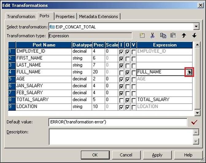
Once you disable the input ports of FULL_NAME and TOTAL_SALARY, you will be able to write the function for the port.

Using the expression editor

To manipulate the date, we need to write the functions in the ports. You can use the functions provided from the list of functions inside the expression editor:

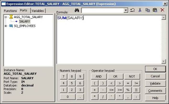
1. Click on the icon shown in the following screenshot to open the expression editor.

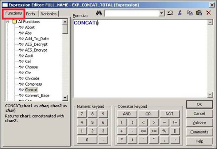
2. New windows where you can write the function will pop up . From the Functions tab, you can use these functions. Informatica PowerCenter provides all the functions that cater to the need of SQL/Oracle functions, mathematical functions, trigonometric functions, date functions, and so on.

In our scenario, we need to use the CONCAT function. Double-click on the Concat function under the list of functions to get the function in the editor, as shown in the following screenshot:

3. Click on Ports in the expression editor, and double-click on FIRST_NAME and LAST_NAME to get the function, as shown in the following screenshot:

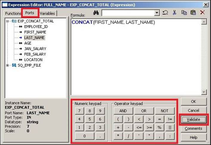
As you can see in the preceding screenshot, the expression editor provides Numeric keypad and Operator keypad, which can be used to write the functions.

Once you finish writing the function, click on Validate to make sure the function is correct syntactically. Then, click on OK.

Similarly, write the function to calculate TOTAL_SALARY; the function will be JAN_SAL+FEB_SAL.

4. Link the corresponding ports to the target, as shown in the following screenshot:

Save the mapping to save the metadata in the repository. With this, we are done creating the mapping using the Expression transformation. We have also learned about ports and how to use an expression editor. We discovered how to write functions in a transformation. These details will be used across all other transformations in Informatica.

The Aggregator transformation

The Aggregator transformation is used for calculations using aggregate functions in a column as opposed to the Expression transformation that is used for row-wise manipulation.

You can use aggregate functions, such as SUM, AVG, MAX, and MIN, in the Aggregator transformation.

Use the EMPLOYEE Oracle table as the source and get the sum of the salaries of all employees in the target.

Perform the following steps to implement the functionality:

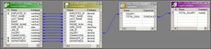
1. Import the source using the EMPLOYEE Oracle table in Source Analyzer and create the TGT_TOTAL_SALARY target in Target Designer.

2. Create the m_AGG_TOTAL_SALARY mapping and drag the source and target from the navigator to the workspace. Create the Aggregator transformation with the AGG_TOTAL_SAL name.

3. As we need to calculate TOTAL_SALARY, drag only the SALARY column from the source qualifier to the Aggregator transformation.

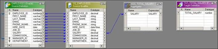
4. Add a new TOTAL_SALARY column to the Aggregator transformation to calculate the total salary, as shown in the following screenshot:

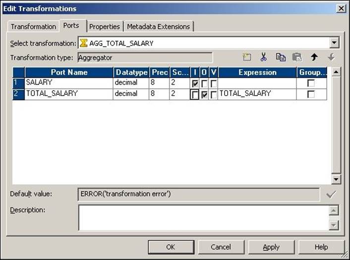
5. Add the function to the TOTAL_SALARY port by opening the expression editor, as described in the preceding section. The function we need to add to get the total salary is SUM(JAN_SAL).

6. Connect the TOTAL_SALARY port to the target, as shown in the following screenshot:

With this, we are done using the Aggregator transformation. When you use the Aggregator transformation, Integration Service temporarily stores the data in the cache memory. The cache memory is created because the data flows in a row-wise manner in Informatica and the calculations required in the Aggregator transformation are column-wise. Unless we temporarily store the data in the cache, we cannot calculate the result. In the preceding scenario, the cache starts storing the data as soon as the first record flows into the Aggregator transformation. The cache will be discussed in detail later in the chapter in the Lookup transformation section.

In the next section, we will talk about the added features of the Aggregator transformation. The Aggregator transformation comes with features such as group by and sorted input.

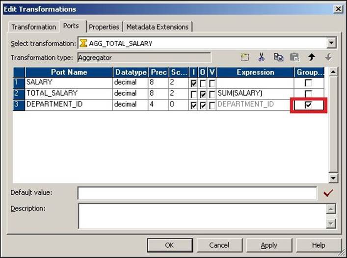
Using Group By

Using the Group By option in the Aggregator transformation, you can get the result of the aggregate function based on groups. Suppose you wish to get the sum of the salaries of all employees based on Department_ID, we can use the group by option to implement the scenario, as shown in the following screenshot:

Using Sorted Input

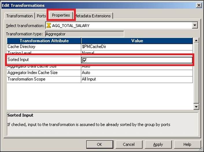
It is always recommended that we pass the Sorted Input to the Aggregator transformation, as this will enhance performance. When you pass the sorted input to the Aggregator transformation, Integration Service enhances the performance by storing less data in the cache. When you pass unsorted data, the Aggregator transformation stores all the data in the cache, which takes more time. When you pass the sorted data to the Aggregator transformation, it stores comparatively less data. The aggregator passes the result of each group as soon as the data for a particular group is received.

Note that the Aggregator transformation cannot perform the operation of sorting the data. It will only internally sort the data for the purpose of calculations. When you pass the sorted data to the Aggregator transformation, check the Sorted Input option in the properties, as shown in the following screenshot:

With this we have seen various option and functionality of Aggregator transformation.

The Sorter transformation

Sorter transformation is used to sort the data in an ascending or descending order based on single or multiple keys. A sample mapping showing Sorter transformation is displayed in the following screenshot:

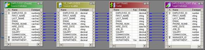
In this mapping, we wish to sort the data based on the DEPARTMENT_ID field. To achieve this, mark the key port for the DEPARTMENT_ID columns in the Sorter transformation and select from the drop-down list what you wish to have as the Ascending or Descending sorting, as shown in the following screenshot:

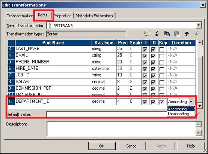
If you wish to sort the data in multiple columns, check the Key ports corresponding to the required port.

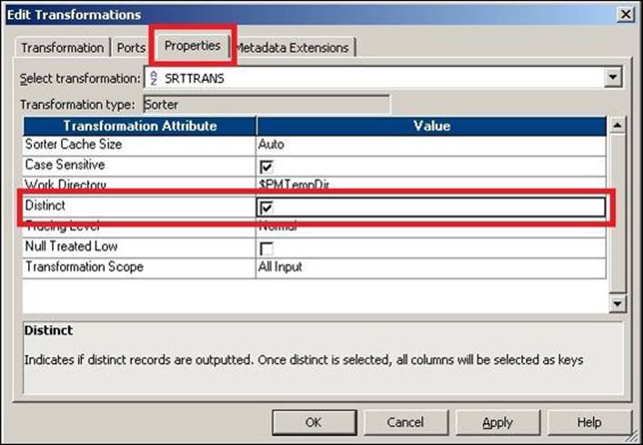
Apart from ordering the data in ascending or descending order, you can also use the Sorter transformation to remove duplicates from the data using the Distinct option in the properties. The sorter can remove duplicates only if the complete record is a duplicate and not just a particular column. To remove a duplicate, check the Distinct option in the Sorter transformation, as shown in the following screenshot:

The Sorter transformation accepts the data in a row-wise manner and stores the data in the cache internally. Once all the data is received, it sorts the data in ascending or descending order based on the condition and sends the data to the output port.

The Filter transformation

Filter transformation is used to remove unwanted records from the mapping. You can define the filter condition in the Filter transformation, and based on the filter condition, the records will be rejected or passed further in the mapping.

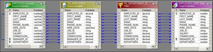
A sample mapping showing the Filter transformation is given in the following screenshot:

The default condition in Filter transformation is TRUE. Based on the condition defined, if the record returns TRUE, the Filter transformation allows the record to pass. For each record that returns FALSE, the Filter transformation drops the records.

To add the Filter transformation, double-click on the Filter transformation and click on the Properties tab, as shown in the following screenshot:

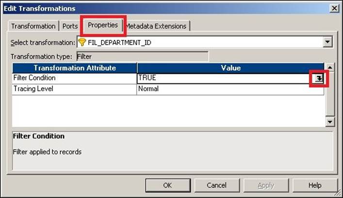
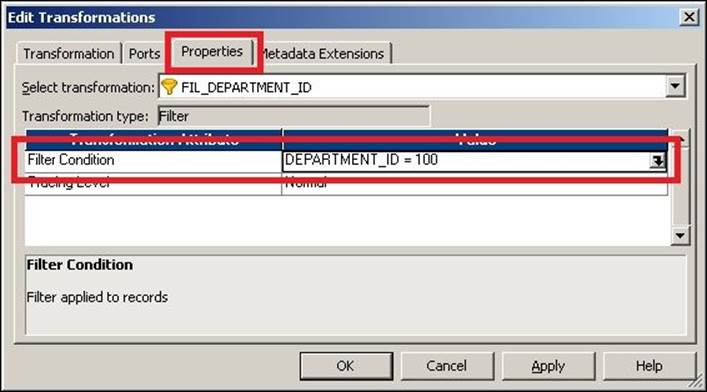
Click on the button shown in the preceding screenshot to open the expression editor and add the function for the filter condition. Then, add the required condition. We have used the condition as DEPARTMENT_ID=100; this will allow records with DEPARTMENT_ID as 100 to reach the target, and the rest of the records will get filtered.

We have understood the functionality of Filter transformation in the above section and next we will talk about Router transformation, which can be used in place of multiple filters.

The Router transformation

Router transformation is single input to multiple output group transformation. Routers can be used in place of multiple Filter transformations. Router transformations accept the data through an input group once, and based on the output groups you define, it sends the data to multiple output ports. You need to define the filter condition in each output group.

A mapping using the Router transformation where we wish to load all records from LOCATION as INDIA in one target, records from UK in another target, and all other nonmatching records in the third target, is indicated in the following screenshot:

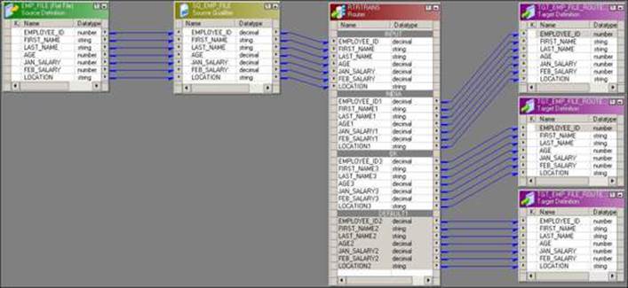
When you drag the columns to the router, the Router transformation creates an input group with only input ports and no output port. To add the output groups, click on the Groups tab and add two new groups. Enter the name of each group under the group name and define the filter condition for each group. Click on OK to create the output groups in the Router transformation.

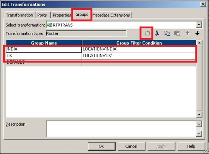
When you add the group, a DEFAULT group gets created automatically. All nonmatching records from the other groups will pass through the default group if you connect the DEFAULT group's output ports to the target.

When you pass the records to the Router transformation through the input group, the Router transformation checks the records based on the filter condition you define in each output group. For each record that matches, the condition passes further. For each record that fails, the condition is passed to the DEFAULT group.

As you can see, Router transformations are used in place of multiple Filter transformations. This way, they are used to enhance the performance.

The Rank transformation

The Rank transformation is used to get a specific number of records from the top or bottom. Consider that you need to take the top five salaried employees from the EMPLOYEE table. You can use the Rank transformation and define the property. A sample mapping indicating the Rank transformation is shown in the following screenshot:

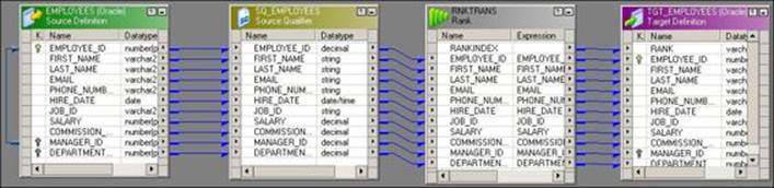
When you create a Rank transformation, a default RANKINDEX output port comes with the transformation. It is not mandatory to use the RANKINDEX port. We have connected the RANKINDEX port to the target as we wish to give the rank of EMPLOYEES based on their SALARY.

When you use a Rank transformation, you need to define the port on which you wish to rank the data. As shown in the following screenshot, we have ranked the data based on SALARY:

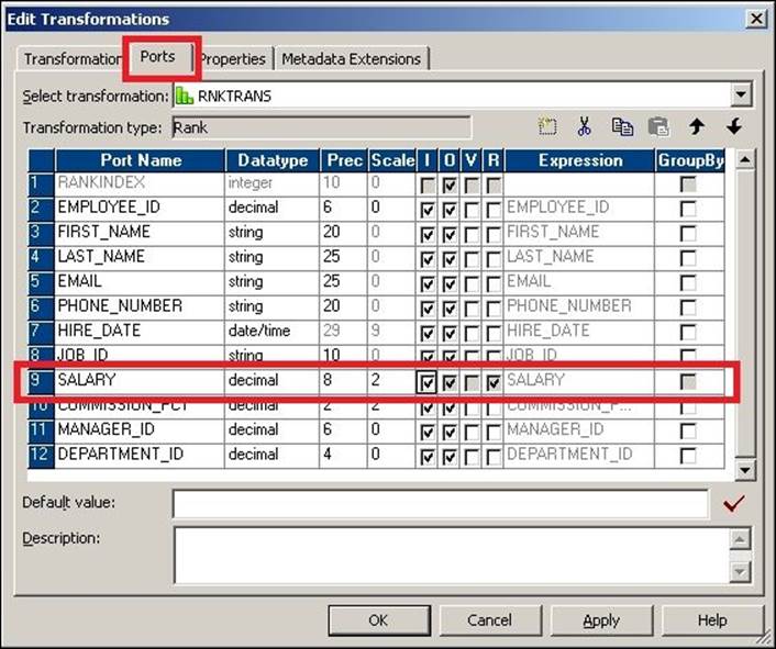
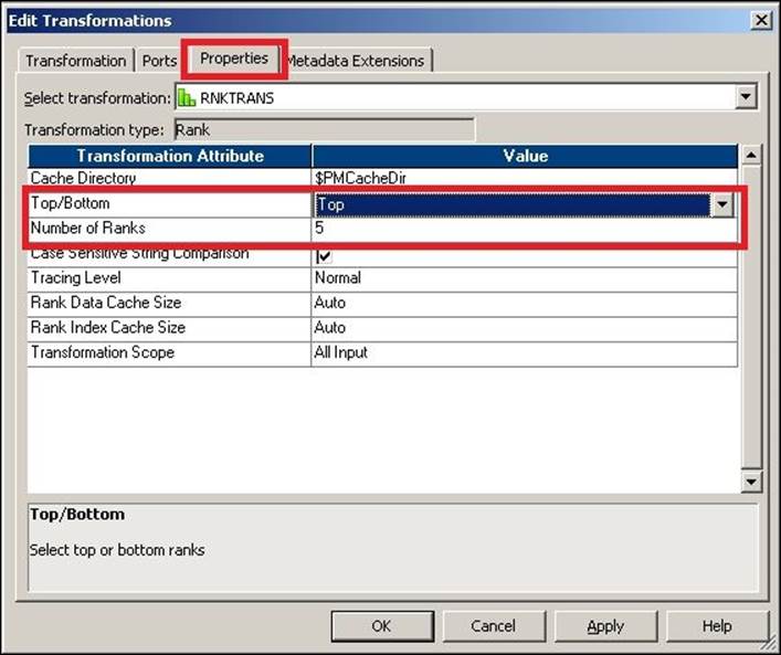
You cannot rank the data on multiple ports. Also, you need to define either the Top or Bottom option and the number of records you wish to rank in the Properties tab. In our case, we have selected Top and 5 to implement the scenario, as shown in the following screenshot:

Rank transformations accept the data in a row-wise manner and store the data in the cache. Once all the data is received, it checks the data based on the condition and sends the data to the output port.

Rank transformations allow you to get the data based on a particular group. In the next section, we will talk about the group by key present in the Rank transformation.

Group by ranking

Rank transformation also provides a feature to get the data based on a particular group. Consider the scenario discussed previously. We need to get the top five salaried employees from each department. To achieve the functionality, we need to select the group by option, as shown in the following screenshot:

Next, we will talk about the default port of Rank transformations, rank index.

Rank index

When you create a Rank transformation, a default column called rank index gets created. If required, this port can generate numbers indicating the rank. This is an optional field that you can use if required. If you do not wish to use rank index, you can leave the port unconnected.

Suppose you have the following data belonging to the SALARY column in the source:

Salary

100

1000

500

600

1000

800

900

When you pass the data through a Rank transformation and define a condition to get the top five salaried records, the Rank transformation generates the rank index as indicated here:

Rank_Index, Salary

1,1000

1,1000

3,900

4,800

5,600

As you can see, the rank index assigns 1 rank to the same salary values, and 3 to the next salary. So if you have five records with 1000 as the salary in the source along with other values, and you defined conditions to get the top five salaries, Rank transformation will give all five records with a salary of 1000 and reject all others.

With this, we have learned all the details of Rank transformation.

The Sequence Generator transformation

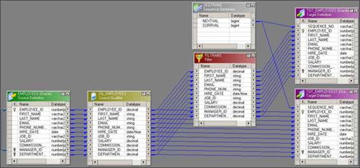
Sequence Generator transformation is used to generate a sequence of unique numbers. Unique values are generated based on the property defined in the Sequence Generator transformation. A sample mapping showing the Sequence Generator transformation is shown in the following screenshot:

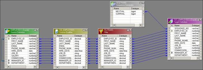
As you can see in the mapping, the Sequence Generator transformation does not have any input port. You need to define the start value, increment by value, and end value in the properties. Based on properties, the sequence generator generates the value. In the preceding mapping, as soon as the first record enters the target from the Source Qualifier transformation, NEXTVAL generates its first value, and so on for other records. The sequence generator is built to generate numbers.

Ports of the Sequence Generator transformation

The Sequence Generator transformation has only two ports, NEXTVAL and CURRVAL. Both the ports are output ports. You cannot add or delete any port in a sequence generator. It is recommended that you always use the NEXTVAL port first. If the NEXTVAL port is utilized, then use the CURRVAL port. You can define the value of CURRVAL in the properties of the Sequence Generator transformation.

Consider a scenario where we are passing two records to the transformation. The following events occur inside the Sequence Generator transformation. Also note that in our case, we have defined the start value as 0, the increment by value as 1, and the end value is the default in the property. Also, the current value defined in Properties is 1. The following is the sequence of events:

1. When the first record enters the target from the filter transformation, the current value, which is set to 1 in the Properties of the sequence generator, is assigned to the NEXTVAL port. This gets loaded into the target by the connected link. So for the first record, SEQUENCE_NO in the target is given the value of 1.

2. The sequence generator increments CURRVAL internally and assigns that value to the current value, 2 in this case.

3. When the second record enters the target, the current value that is set as 2 now gets assigned to NEXTVAL. The sequence generator gets incremented internally to give CURRVAL a value of 3.

So at the end of the processing of record 2, the NEXTVAL port will have a value of 2 and the CURRVAL port will have its value set as 3. This is how the cycle keeps on running till you reach the end of the records from the source.

It is slightly confusing to understand how the NEXTVAL and CURRVAL ports behave, but after reading the given example, you will have a proper understanding of the process.

Properties of the Sequence Generator transformation

There are multiple values that you need to define inside the Sequence Generator transformation. Double-click on the sequence generator and click on the Properties tab, as shown in the following screenshot:

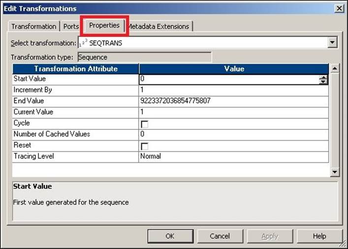
Let's discuss the properties in detail:

· Start Value: This comes into the picture only if you select the Cycle option in the properties. Start Value indicates the Integration Service that starts over from this value when the end value is reached after you have checked the cycle option.

The default value is 0 and the maximum value is 9223372036854775806.

· Increment By: This is the value by which you wish to increment the consecutive numbers from the NEXTVAL port.

The default value is 1 and the maximum value is 2147483647.

· End Value: This is the maximum value that the Integration Service can generate. If the Sequence Generator reaches the end value and is not configured for the cycle, the session will fail, giving the data overflow error. The maximum value is 9223372036854775807.

· Current Value: This indicates the value assigned to the CURRVAL port. Specify the current value that you wish to have as the value for the first record. As mentioned earlier, the CURRVAL port gets assigned to NEXTVAL, and the CURRVAL port is incremented.

The CURRVAL port stores the value after the session is over, and when you run the session the next time, it starts incrementing the value from the stored value if you have not checked the reset option. If you check the reset option, Integration Services resets the value to 1. Suppose you have not checked the Reset option and you have passed 17 records at the end of the session; then, the current value will be set to 18, which will be stored internally. When you run the session the next time, it starts generating the value from 18.

The maximum value is 9223372036854775807.

· Cycle: If you check this option, Integration Service cycles through the sequence defined. If you do not check this option, the process stops at the defined End Value.

If your source records are more than the end value defined, the session will fail with an overflow error.

· Number of Cached Values: This option indicates how many sequential values Integration Services can cache at a time. This option is useful only when you are using reusable Sequence Generator transformations.

The default value for nonreusable transformations is 0. The default value for reusable transformations is 1000. The maximum value is 9223372036854775807.

· Reset: If you do not check this option, Integration Service stores the value of the previous run and generates the value from the previously stored value. Otherwise, the integration will get reset to the defined current value and will generate values from the initial value that was defined. This property is disabled for reusable Sequence Generator transformations.

· Tracing Level: This indicates the level of detail you wish to write into the session log. We will discuss this option in detail later in the chapter.

With this, we have seen all the properties of the Sequence Generator transformation.

Let's talk about the usage of the Sequence Generator transformation:

· Generating a primary/foreign key: The sequence generator can be used to generate a primary key and foreign key. The primary key and foreign key should be unique and not null. The Sequence Generator transformation can easily do this, as seen here. Connect the NEXTVAL port to the targets for which you wish to generate the primary and foreign key, as shown in the following screenshot:

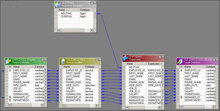
· Replace the missing values: You can use the Sequence Generator transformation to replace missing values by using IIF and ISNULL functions. Consider that you have some data with JOB_ID of an employee. Some records do not have JOB_ID in the table. Use the following function to replace these missing values. Make sure you are not generating NEXTVAL in a manner similar to existing JOB_ID in the data:

· IIF( ISNULL (JOB_ID), NEXTVAL, JOB_ID)

The preceding function interprets whether JOB_ID is null and then assigns NEXTVAL, otherwise it keeps JOB_ID as it is. The following screenshot indicates these requirements:

With this, we have learned all the options available in the Sequence Generator transformation. Next, we will talk about Joiner transformations.

The Joiner transformation

Joiner transformation is used to join two heterogeneous sources. You can join data from the same source type as well. The minimum criteria to join the data are matching columns in both the sources. A mapping indicating the Joiner transformation is shown in the following screenshot:

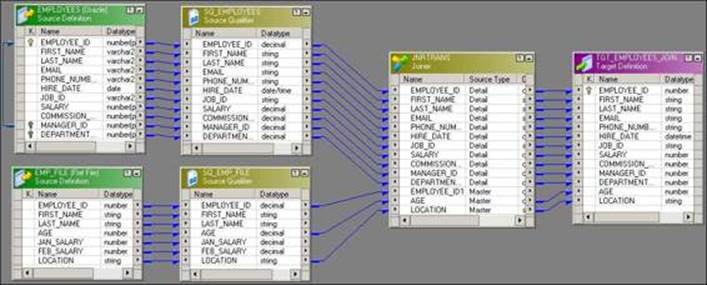
A Joiner transformation has two pipelines; one is called master and the other is called detail. One source is called the master source and the other is called detail. We do not have left or right joins like we have in the SQL database.

To use a Joiner transformation, drag all the required columns from two sources into the Joiner transformation and define the join condition and join type in the properties.

Master and detail pipeline

As mentioned in the preceding section, one source is called master and the other is called detail. By default, when you add the first source, it becomes the detail and the other becomes the master. You can decide to change the master or detail source. To make a source the master, check theMaster port for the corresponding source, as shown in the following screenshot:

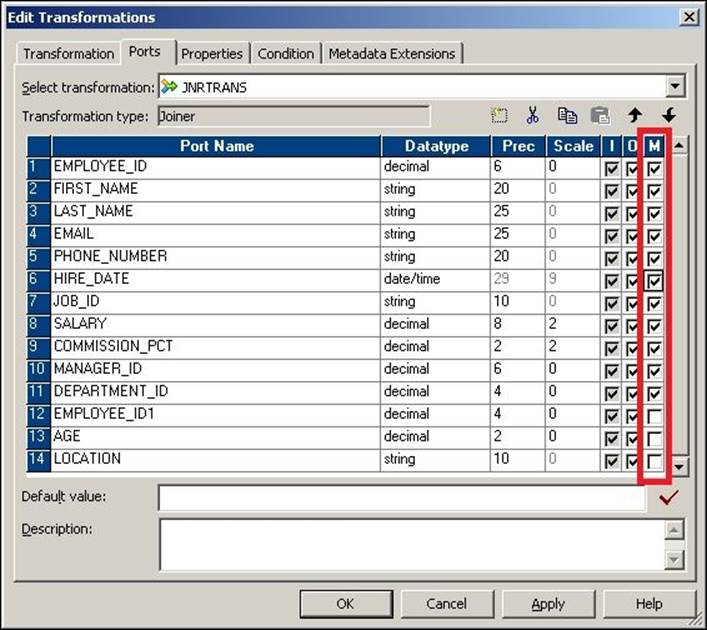
Always verify that the master and detail sources are defined to enhance the performance. It is always recommended that you create a table with a smaller number of records as the master and the other as the detail. This is because Integration Service picks up the data from the master source and scans the corresponding record in the details table. So if we have a smaller number of records in the master table, fewer iterations of scanning will happen. This enhances the performance.

Join condition

Join conditions are the most important condition to join the data. To define the join condition, you need to have a common port in both the sources. Also, make sure the data type and precision of the data you are joining is same. You can join the data based on multiple columns as well. Joining the data on multiple columns increases the processing time. Usually, you join the data based on key columns such as the primary key/foreign key of both the tables.

Joiner transformations do not consider NULL as matching data. If it receives NULL in the data, it does not consider them to be matching.

To define a join condition, double-click on the Joiner transformation, click on the Condition tab, and define the new condition.

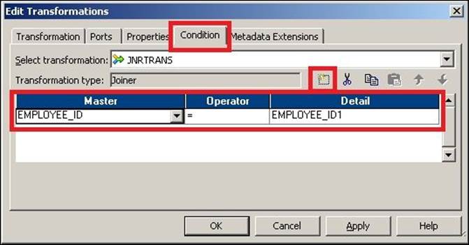
You can define multiple conditions to join two tables.

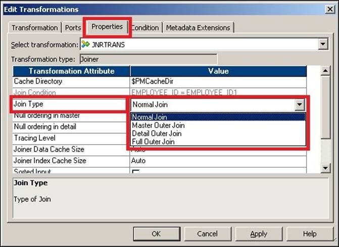
Join type

The Joiner transformation matches the data based on the join type defined. Similar to SQL, Joiner transformation use the join type to join the data. Let's discuss the join type in detail by taking the following example. We have two sources, the master source as EMPLOYEE_TABLE and the detail source as EMPLOYEE_FILE:

EMPLOYEE_TABLE (Master Source – Oracle`)

EMPLOYEE_ID,AGE

101,20

102,30

103,20

EMPLOYEE_FILE (Detail Source – Flat File)

EMPLOYEE_ID,SAL

101,1000

103,4000

105,2000

106,4000

110,5000

As you can see, we have created a table with fewer records as the master source to enhance performance. To assign the join type, double-click on the Joiner transformation and click on the Properties tab. Select the join type out of the four types from the drop-down list, as shown in the following screenshot:

Normal join

When you define a normal join, Integration Service allows only matching records from both the master and detail source and discards all other records.

For the preceding scenario, we will set the join condition as EMPLOYEE_ID = EMPLOYEE_ID.

The result of the normal join for the previously-mentioned data is as follows:

EMPLOYEE_ID,AGE,SAL

101,20,1000

103,20,4000

All nonmatching records with a normal join will get rejected.

Full join

When you define a full join, Integration Service allows all the matching and nonmatching records from both the master and detail source.

The result of the full join for the previously mentioned data is as follows:

EMPLOYEE_ID,AGE,SAL

101,20,1000

102,30,NULL

103,20,4000

105,NULL,2000

106,NULL,4000

110,NULL,5000

Master outer join

When you define a master outer join, Integration Service allows all matching records from both the master and detail source and also allows all other records from the details table.

The result of the master outer join for the previously mentioned data is as follows:

EMPLOYEE_ID,AGE,SAL

101,20,1000

103,20,4000

105,NULL,2000

106,NULL,4000

110,NULL,5000

Detail outer join

We you define a detail outer join, Integration Service allows all matching records from both the master and detail source and also allows all other records from the master table.

The result of the detail outer join for the previously mentioned data is as follows:

EMPLOYEE_ID,AGE,SAL

101,20,1000

102,30,NULL

103,20,4000

With this, we have learned about the various options available in Joiner transformations.

Union transformation

The Union transformation is used to merge data from multiple sources. Union is a multiple input, single output transformation. It is the opposite of router transformations, which we discussed earlier. The basic criterion to use a Union transformation is that you should have data with the matching data type. If you do not have data with the matching data type coming from multiple sources, the Union transformation will not work. The Union transformation merges the data coming from multiple sources and does not remove duplicates, so it acts as the union of all SQL statements.

As mentioned, union requires data to come from multiple sources. Union reads the data concurrently from multiple sources and processes the data. You can use heterogeneous sources to merge the data using a Union transformation.

A mapping indicating the Union transformation is shown in the following screenshot:

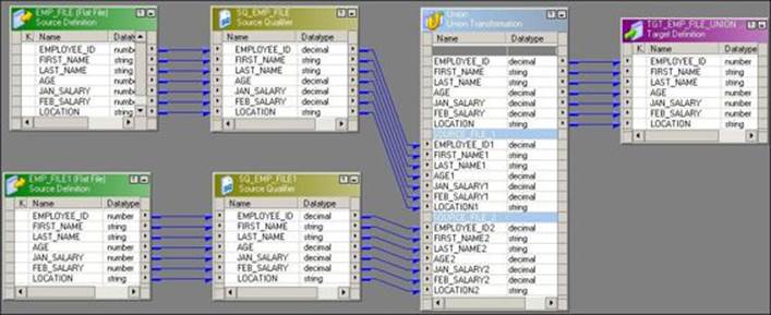
Working on Union transformation is a little different from other transformations. To create a Union transformation, perform the following steps:

1. Once you create a Union transformation, drag all the required ports from one source to the Union transformation. As soon you drag the port, the union creates an input group and also creates another output group with the same ports as the input.

2. Add the output groups from the Group tab in the Union transformation. Add as many groups as the input sources you have, as shown in the following screenshot:

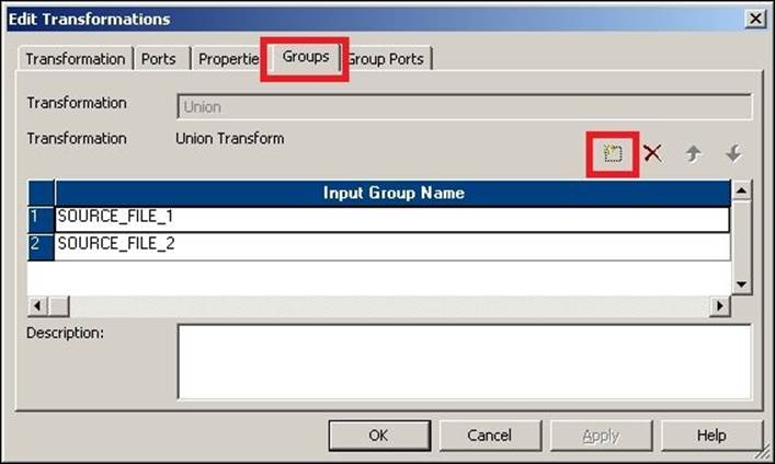
3. Once you add the groups, the Union transformation creates the groups with the same ports, as shown in the preceding mapping.

4. Link the ports from the other source to the input ports of the other group in the Union transformation.

With this, we have created a mapping using a Union transformation.

Source Qualifier transformation

Source Qualifier transformation act as virtual sources in Informatica. When you drag a relational table or flat file in Mapping Designer, the Source Qualifier transformation comes along with it. A source qualifier is the point where the Informatica processing actually starts. The extraction process starts from the source qualifier.

Note that it is always recommended that the columns of source and source qualifier match. Do not change the columns or their data type in the source qualifier. You can note the data type difference in the source definition and source qualifier, which is because Informatica interprets the data in that way itself.

To discuss the source qualifier, let's take an example of the Joiner transformation mapping we created earlier.

As you can see, there are two Source Qualifier transformations present in the mapping: one for flat file and the other for a relational database. You can see that we have connected only three columns from the Source Qualifier transformation of flat file to the Joiner transformation. To reiterate the point, all the columns are dragged from the source to source qualifier, and only three columns are linked to the Joiner transformation. This indicates that the source qualifier will only extract data that's related to three ports, not all. This helps in improving performance, as we are not extracting the unwanted columns' data.

In the same mapping, another Source Qualifier transformation is connected to a relational source. Multiple options are possible in this case. We will discuss each option in detail in the upcoming sections.

Viewing the default query

When you use the relational database as a source, the source qualifier generates a default SQL query to extract the data from the database table. By default, Informatica extracts all the records from the database table. To check the default query generated by Informatica, perform the following steps:

1. Double-click on the Source Qualifier transformation, click on the Properties tab, and select the SQL query.

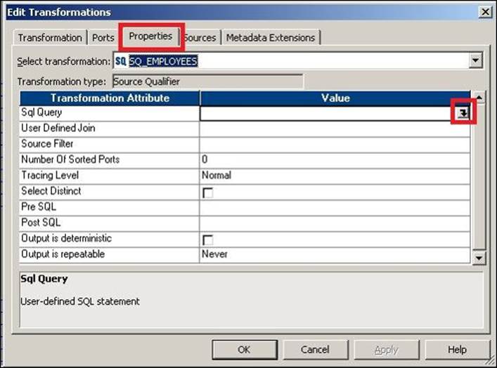
2. The SQL editor opens up. Click on the Generate SQL option. If required, specify the database username and password.

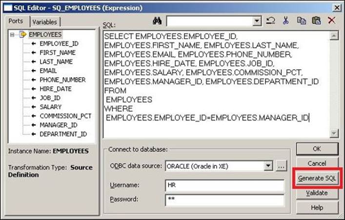
Informatica shows you the default query based on the links connected from the Source Qualifier transformation.

In the preceding screenshot, the WHERE clause in the SQL query (WHERE EMPLOYEES.EMPLOYEE_ID = EMPLOYEES.MANAGER_ID) signifies the self-referential integrity of the table. That means that every manager needs to be an employee.

Overriding the default query

We can override the default query generated by the Source Qualifier transformation. If you override the default query generated by the source qualifier, it is called an SQL override. You should not change the list of ports or the order of the ports in the default query. You can write a new query or edit the default query generated by Informatica. You can perform various operations while overriding the default query.

Using the WHERE clause

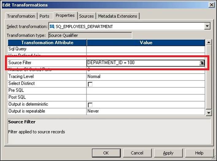
You can add the WHERE clause in the SQL query while you override the default query. When you add the WHERE clause, you reduce the number of records extracted from the source. This way, we can say that our Source Qualifier transformation is acting as a filter transformation. You can also define the WHERE condition in the source filter. If you define the source filter, you need not add the WHERE clause in the SQL query. You can add the source filter as shown in the following screenshot:

Joining the source data

You can use the Source Qualifier transformation to define the user-defined join types. When you use this option, you can avoid using the Joiner transformation in the mapping. When you use the Source Qualifier transformation to join the data from two database tables, you will not use the master or detail join. You will use the database-level join types, such as the left and right join.

We will use the EMPLOYEE and DEPARTMENT Oracle tables to join the data using the Source Qualifier transformation. Follow these steps to use the source qualifier to perform the join functionality:

1. Open Mapping Designer and drag the EMPLOYEE and DEPARTMENT Oracle tables into the mapping. Once you drag both the sources into Mapping Designer, delete the source qualifier of the DEPARTMENT table and drag all the columns from the DEPARTMENT source definition into the EMPLOYEEsource qualifier, as shown in the following screenshot:

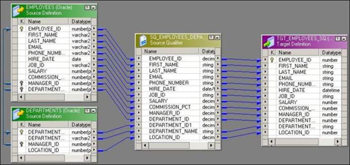
Link the required columns from the source qualifier to the target as per your requirement.

2. Open the Properties tab of the Source Qualifier transformation and generate the default SQL. Now, you can modify the default generated query as per your requirement, to perform the join on the two tables.

Using this feature helps make our mapping simple by avoiding the Joiner transformation and, in turn, helps in faster processing. Note that you cannot always replace a joiner with a source qualifier. This option can be utilized only if you wish to join the data at the source level and both your sources are relational tables in the same database and connection. You can use a single source qualifier to join the data from multiple sources; just make sure the tables belong to same database scheme.

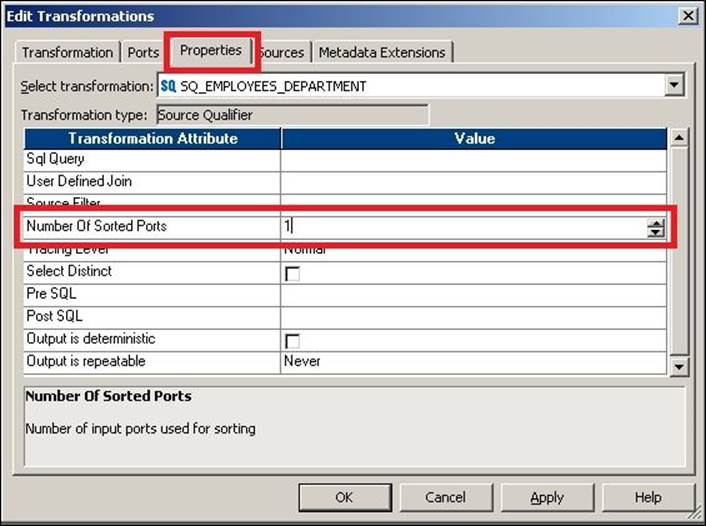
Sorting the data

You can also use the Source Qualifier transformation to sort the data while extracting the data from the database table. When you use the sorted port option, Integration Service will add defined ports to the ORDER BY clause in the default query. It will keep the sequence of the ports in the query similar to the sequence of ports defined in the transformation. To sort the data, double-click on the Source Qualifier transformation, click on the Properties tab, and specify Number Of Sorted Ports, as shown in the following screenshot:

This will be possible only if your source is a database table and only if you wish to sort the data at the source level. If you wish to sort the data in between the mapping, you need to apply the Sorter transformation.

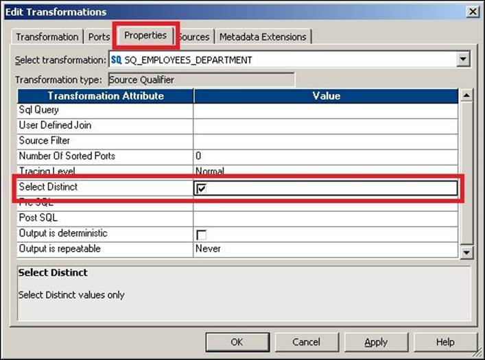
Selecting distinct records

You can use the source qualifier to remove the duplicates from the database tables using the select distinct option. By default, Integration Service extracts all the columns from the source in the default query. When you select the distinct option, Integration Service adds the SELECT DISTINCTstatement into the query that it generates.

To add the distinct command in your query, double-click on the Source Qualifier transformation, click on the Properties tab, and check the Select Distinct option, as shown in the following screenshot:

This will be possible only if your source is a database table and only if you wish to select unique records at the source level. If you wish to get unique records in between the mapping, you need to use the Sorter transformation, which also provides the ability to remove duplicates.

Classification of transformations

At this point, we have seen quite a few transformations and their functions. Before we look at the next transformations, let's talk about the classification of transformations. Based on their functionality, transformations are divided as follows.

Active and passive

This classification of transformations is based on the number of records in the input and output port of the transformation. This classification is not based on the number of ports or the number of groups.

If the transformation does not change the number of records in its input and output ports, it is said to be a passive transformation. If the transformation changes the number of records in the input and output ports of the transformation, it is said to be an active transformation. Also, if the transformation changes the sequence of records passing through it, it is classed as an active transformation, as with Union transformations. Let's take an example to understand this classification.

Consider the Expression transformation from the mapping we used in the example of Expression transformations, where we concatenated FIRST_NAME and LAST_NAME, as shown in the following screenshot:

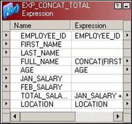
As you can see, the number of input ports is seven and the number of output ports is five. Say our source contains 10 records in the mapping. When we pass all the records to the transformation, the total records that will reach the input ports will be 10 and the total records that will reach the output ports will also be 10, so this makes Expression transformation passive. We are not concerned about the number of ports in the input and output.

Consider the example of filter transformations that filter out unwanted records, as this changes the number of records, it is an active transformation.

Connected and unconnected

A transformation is said to be connected if it is connected to any source, target, or any other transformation by at least one link. If the transformation is not connected by any link, it it classified as unconnected. Only the lookup and Stored Procedure transformations can be connected and unconnected, all other transformations are connected.

The Lookup transformation

The Lookup transformation is used to look up a source, source qualifier, or target to get the relevant data. You can look up flat file and relational tables. The Lookup transformation works on similar lines as the joiner, with a few differences. For example, lookup does not require two sources. Lookup transformations can be connected and unconnected. They extract the data from the lookup table or file based on the lookup condition.

Creating a Lookup transformation

Perform the following steps to create and configure a Lookup transformation:

1. In Mapping Designer, click on Transformations and create a Lookup transformation. Specify the name of the Lookup transformation and click on OK.

2. A new window will ask you to select Source, Target, or Source Qualifier that you wish to look up. You will get a list of all the sources, targets, and source qualifiers available in your repository. Click on the required component and then click on OK, as shown in the following screenshot:

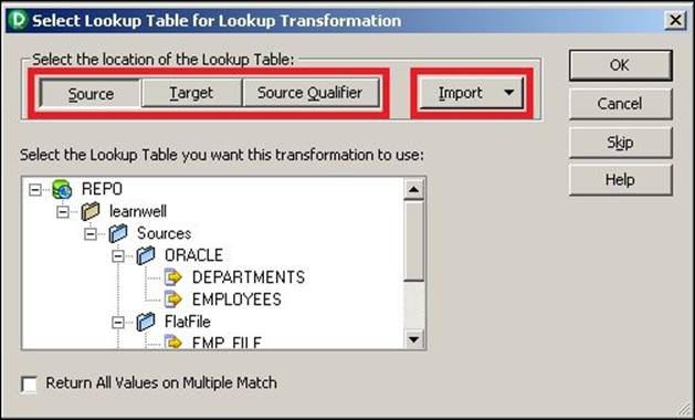
If the required source or target is not available in the repository, you can import it before you use it to look up. Click on the Import button to import the structure, as shown in the preceding screenshot.

The Lookup transformation with the same structure as the source, target, or source qualifier appears in the workspace.

Configuring the Lookup transformation

We have learned how to create a Lookup transformation in the previous section. Now we will implement a mapping similar to the one shown in the Joiner transformation using the Lookup transformation. We will use the EMPLOYEE Oracle table as the source and will look up the EMP_FILE flat file. Perform the following steps to implement the mapping:

1. Drag the EMPLOYEE table as the source in Mapping Designer and drag the target.

2. We have already created the Lookup transformation.

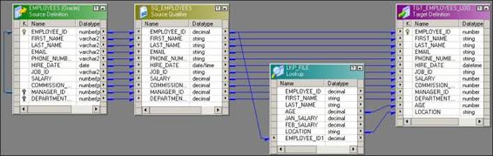
3. To get the relevant data based on the matching conditions of the EMPLOYEE table and the EMP_FILE file, drag the EMPLOYEE_ID column from the EMPLOYEE table to the Lookup transformation. Drag the corresponding columns from the EMPLOYEE source qualifier and Lookup transformation to the target, as shown in the following screenshot:

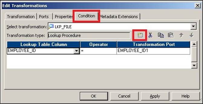
4. Click on the Condition tab and create a new condition, as shown in the following screenshot:

Setting up the Lookup transformation

When you create the Lookup transformation, you can configure it to cache the data. Caching the data makes the processing faster, as the data is stored internally after the cache is created. Once you choose to cache the data, the Lookup transformation caches the data from the file or table once. Then, based on the condition defined, the lookup sends the output value. As the data gets stored internally, processing becomes faster as it does not need to check the lookup condition in the file or database. Integration Service queries the cache memory instead of checking the file or table to fetch the required data.

When you choose to create the cache, Integration Service creates cache files in the $PMCacheDir default directory. The cache is created automatically and is also deleted automatically once the processing is complete. We will discuss what cache is later in the chapter.

Lookup ports

A Lookup transformation has four different types of ports. To view the ports of the Lookup transformation, click on its Ports tab.

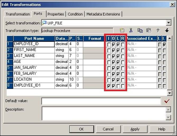
The ports are as follows:

· Input Ports (I): The input ports receive the data from other transformations. This port will be used in the lookup condition. You need to have at least one input port.

· Output Port (O): Output ports pass the data from the Lookup transformation to other transformations.

· Lookup Port (L): Each column is assigned as the lookup and output port when you create the Lookup transformation. If you delete the lookup port from the flat file lookup source, the session will fail. If you delete the lookup port from the relational lookup table, Integration Service extracts the data with only the lookup port. This helps to reduce the data extracted from the lookup source.

· Return Port (R): This is only used in the case of an unconnected Lookup transformation. It indicates which data you wish to return in the Lookup transformation. You can define only one port as the return port, and it's not used in the case of connected Lookup transformations.

Lookup queries

Similar to the Source Qualifier transformation, which generates a default query when you use the source as a relational database table, the Lookup transformation also generates a default query based on the ports used in the Lookup transformation. To check the default query generated by the Lookup transformation, click on the Properties tab and open Lookup Sql Override, as shown in the following screenshot:

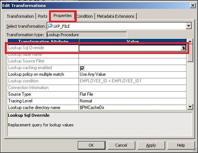
Similar to overriding the default SQL in the Source Qualifier transformation, you can override the default query generated by the Lookup transformation. If you override the default query generated by the Lookup transformation, it is referred to as a lookup SQL override.

Unconnected Lookup transformations

As mentioned, unconnected transformations are not connected to any other transformation, source, or target by any links. An unconnected Lookup transformation is called by another transformation with the :LKP function. Using the :LKP function, you can pass the required value to the input port of the Lookup transformation, and the return port passes the output value back to the transformation from which the lookup was called. A mapping using an unconnected Lookup transformation is as follows:

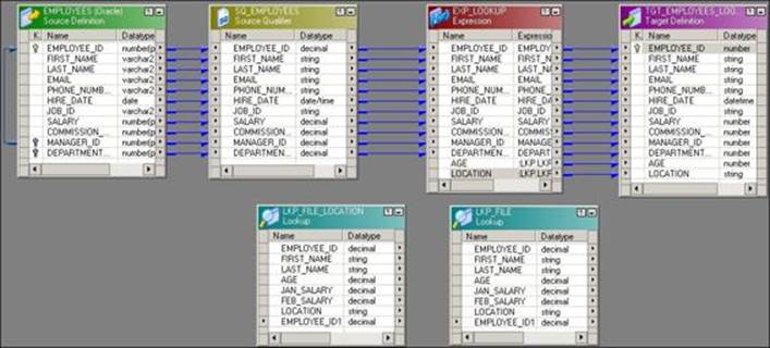
In the preceding mapping, we are implementing the same scenario that we implement using a connected Lookup transformation. Perform the following steps to implement this scenario:

1. Create an Expression transformation and drag all the ports from the Source Qualifier transformation to Expression transformation.

2. Create an EMPLOYEE_ID input port in the Lookup transformation that will accept the value of EMPLOYEE_ID using the :LKP function.

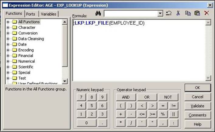
3. Create another AGE output port in the Expression transformation that is used to call an unconnected Lookup transformation using the :LKP function. Link the AGE port to the target. Write the :LKP.LKP_FILE(EMPLOYEE_ID) function in the expression editor of the AGE column, as shown in the following screenshot:

4. Double-click on the Lookup transformation, click on ports, and make AGE the return port, as shown in the following screenshot:

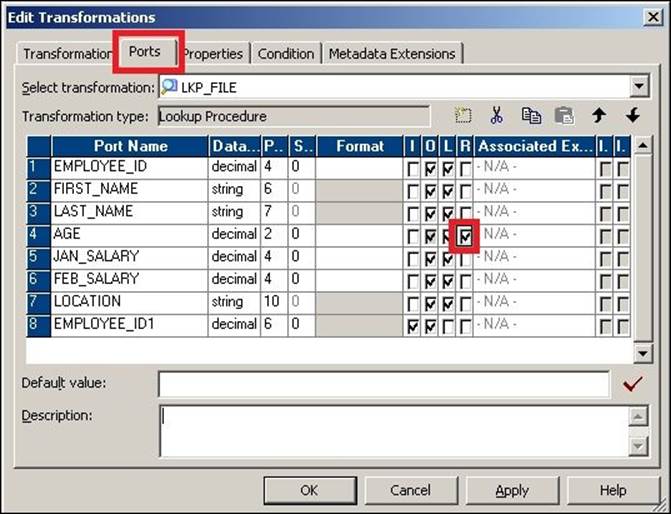
When you execute the mapping, row-wise data will flow from the source to the Expression transformation. The :LKP function passes the data to the Lookup transformation, which compares the data based on the condition defined in the Condition tab, which in turn returns the data from the Return port to the Expression transformation, from where the data is passed further in the mapping.

5. Similarly, add another LOCATION output port to the Expression transformation. Then, create another Lookup transformation. We cannot use the same Lookup transformation, as the unconnected Lookup transformation can return only one port. Follow the process described here to look up for the AGE port to complete the mapping.

We have seen the implementation of connected and unconnected Lookup transformations.

Lookup transformation properties

Let's discuss the properties of the Lookup transformation:

We have now seen all the details of Lookup transformations.

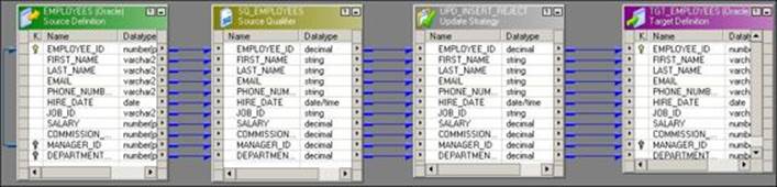
The Update Strategy transformation

Update Strategy transformations are used to INSERT, UPDATE, DELETE, or REJECT records based on the defined condition in the mapping. An Update Strategy transformation is mostly used when you design mappings for slowly changing dimensions. When you implement SCD, you actually decide how you wish to maintain historical data with the current data. We have discussed SCDs in Chapter 3, Implementing SCD – Using Designer Screen Wizards. When you wish to maintain no history, complete history, or partial history, you can achieve this functionality by either using the property defined in the session task or using the Update Strategy transformation.

When you use the session task, you instruct Integration Service to treat all records in the same way, that is, either INSERT, UPDATE, or DELETE.

When you use the Update Strategy transformation in the mapping, the control is no longer with the session task. The Update Strategy transformation allows you to INSERT, UPDATE, DELETE, or REJECT records based on the requirement. When you use the Update Strategy transformation, the control is no longer with the session task. You need to define the following functions to perform the corresponding operations:

· DD_INSERT: This is used when you wish to insert records, which are also represented by the numeral 0

· DD_UPDATE: This is used when you wish to update the records, which are also represented by the numeral 1

· DD_DELETE: This is used when you wish to delete the records, which are also represented by the numeral 2

· DD_REJECT: This is used when you wish to reject the records, which are also represented by the numeral 3

Consider that we wish to implement a mapping using the Update Strategy transformation, which allows all employees with salaries higher than 10000 to reach the target and eliminates all other records. The following screenshot depicts the mapping for this scenario:

Double-click on the Update Strategy transformation and click on Properties to add the condition:

IIF(SALARY >= 10000, DD_INSERT, DD_REJECT)

The Update Strategy transformation accepts the records in a row-wise manner and checks each record for the condition defined. Based on this, it rejects or inserts the data into the target.

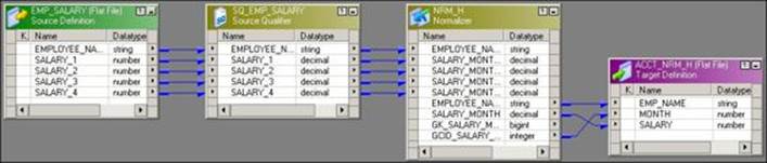
The Normalizer transformation

The Normalizer transformation is used in place of Source Qualifier transformations when you wish to read the data from the cobol copybook source. Also, a Normalizer transformation is used to convert column-wise data to row-wise data. This is similar to the transpose feature of MS Excel. You can use this feature if your source is a cobol copybook file or relational database table. The Normalizer transformation converts columns to rows and also generates an index for each converted row. A sample mapping using the Normalizer transformation is shown in the following screenshot:

Consider the following example, which contains the salaries of three employees for four months:

STEVE 1000 2000 3000 4000

JAMES 2000 2500 3000 3500

ANDY 4000 4000 4000 4000

When you pass the data through the Normalizer transformation, it returns the data in a row-wise form along with the index, as follows:

STEVE 1000 1

STEVE 2000 2

STEVE 3000 3

STEVE 4000 4

JAMES 2000 1

JAMES 2500 2

JAMES 3000 3

JAMES 3500 4

ANDY 4000 1

ANDY 4000 2

ANDY 4000 3

ANDY 4000 4

As you can see, the index key is incremented for each value. It also initializes the index from 1 when processing data for a new row.

Configuring the Normalizer transformation – ports

Normalizer transformation ports are different from other transformations ports. You cannot edit the ports of Normalizer transformations. To define the ports, you need to configure the Normalizer tab of a Normalizer transformation. To add the multiple occurring ports to the Normalizer transformation, double-click on the Normalizer transformation and click on Normalizer. Add the columns to the Normalizer tab. You need to add the single and multiple occurring ports in the Normalizer tab. When you have multiple occurring columns, you need to define them under theOccurs option in the Normalizer transformation, as shown in the following screenshot:

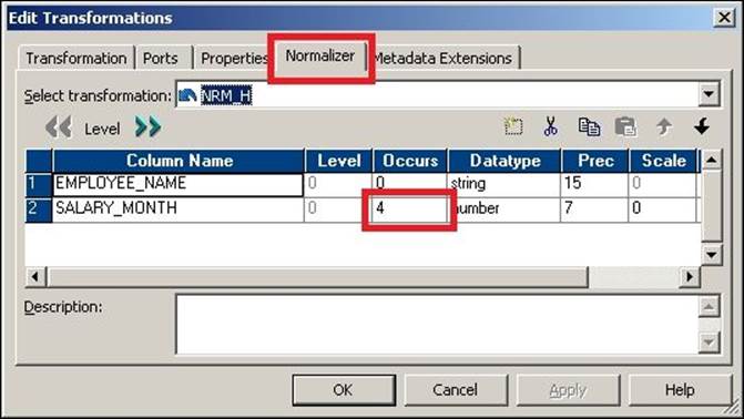
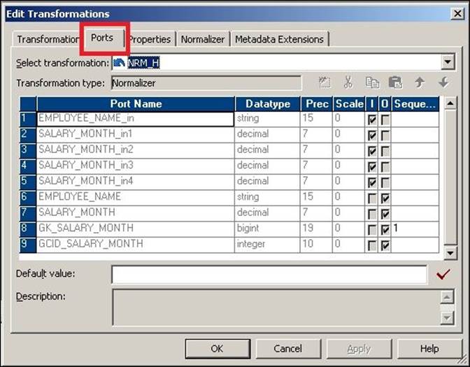
When you add the columns in the Normalizer tab, the columns get reflected in the Ports tab based on the options definitions. In our case, we define SALARY_MONTH under occurs 4 times in the Normalizer transformation. This creates the port four times in the ports tab.

The Normalizer transformation creates a new port called generated column ID (GCID) for every multi-occurring ports you define in the Normalizer tab. In our case, it is created for SALARY_MONTHLY. This port generates the index value to be assigned to new multi-occurring values. The GCID is incremented automatically each time it processes a new record, as shown in the following screenshot:

The attributes of the Normalizer tab are as follows:

The Stored Procedure transformation

It stores procedure database components. Informatica uses the stored procedure in a manner that is similar to database tables. Stored procedures are sets of SQL instructions that require a certain set of input values, and in turn the stored procedure returns output values. This way, you either import or create database tables and import or create the stored procedure in the mapping. To use the stored procedure in mapping, the stored procedure should exist in the database.

Similar to Lookup transformations, stored procedures can also be connected or unconnected transformations in Informatica. When you use a connected stored procedure, you pass the value to stored procedures through links. When you use an unconnected stored procedure, you pass the value using the :SP function.

Importing Stored Procedure transformations

Importing the stored procedure is similar to importing the database tables in Informatica. Earlier, we saw the process of importing database tables. Before you import the stored procedure, make sure the stored procedure is created and tested at the database level. Also, make sure that you have valid credentials to connect to the database.

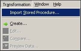
To import the stored procedure, open the mapping in Mapping Designer. Click on Transformation and select the Import Stored Procedure… option, as shown in the following screenshot:

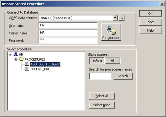
Connect to the database credentials, click on the required procedure, and click on OK.

The stored procedure appears in the workspace. Connect the corresponding input and output ports to complete the mapping.

Creating Stored Procedure transformations

You can create Stored Procedure transformations instead of importing them. Usually, the best practice is to import the stored procedure, as it takes care of all the properties automatically. When you create the transformation, you need to take care of all the input, output, and return ports in the Stored Procedure transformation. Before you create the stored procedure, make sure the stored procedure is created in the database.

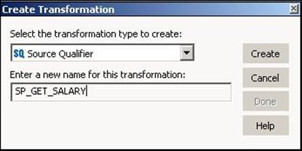
To create the Stored Procedure transformation, open the mapping in Mapping Designer. Navigate to Transformation | Create. Then, select the Stored Procedure transformation from the list of transformations and mention the name of the transformation, as shown in the following screenshot:

In the next window, click on Skip. A Stored Procedure transformation appears in Mapping Designer. Add the corresponding input, output, and variable ports. You need to be aware of the ports present in the stored procedure created in the database.

Using Stored Procedure transformations in the mapping

As mentioned, Stored Procedure transformations can be connected or unconnected. Similar to Lookup transformations, you can configure connected or unconnected Stored Procedure transformations.

Connected Stored Procedure transformations

A connected Stored Procedure transformation is connected in the mapping with the links. The connected Stored Procedure transformation receives data in the input port and sends the data out using output ports. A sample mapping showing the connected Stored Procedure transformation is shown in the following screenshot:

Unconnected Stored Procedure transformations

An unconnected Stored Procedure transformation is not connected to any other source, target, or transformation by links. The unconnected Stored Procedure transformation is called by another transformation using the :SP function. It works in a manner similar to an unconnected Lookup transformation, which is called using the :LKP function.

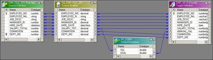
A sample mapping using the unconnected Stored Procedure transformation is shown in the following screenshot:

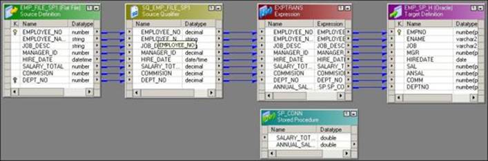
We have used Expression transformations to call the stored procedure. The function that is used to call the stored procedure is SP.SP_CONN(SALARY_TOTAL,PROC_RESULT). Follow the steps similar to ones used for unconnected Lookup transformations in order to create the unconnected stored procedure mapping.

Transaction Control transformations

Transaction Control transformations allow you to commit or roll back individual records based on certain conditions. By default, Integration Service commits the data based on the properties you define at the session task level. Using the Commit Interval property, Integration Service commits or rolls backs the data into the target. Suppose you define Commit Interval as 10,000, Integration Service will commit the data after every 10,000 records. When you use a Transaction Control transformation, you get the control at each record to commit or roll back.

When you use the Transaction Control transformation, you need to define the condition in the expression editor of the Transaction Control transformation. When you run the process, the data enters the Transaction Control transformation in a row-wise manner. The Transaction Control transformation evaluates each row, based on which it commits or rolls back the data.

A sample mapping using the Transaction Control transformation is shown in the following screenshot:

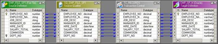
To use the Transaction Control transformation in the mapping, perform the following steps:

1. Open the mapping in Mapping Designer and create the Transaction Control transformation.

2. Drag the required columns from the Source Qualifier transformation to the Transaction Control transformation.

3. Connect the appropriate ports from the Transaction Control transformation to the target.

4. Double-click on the Transaction Control transformation and click on Properties. We need to define the condition in the Transaction Control transformation expression editor, as shown in the following screenshot:

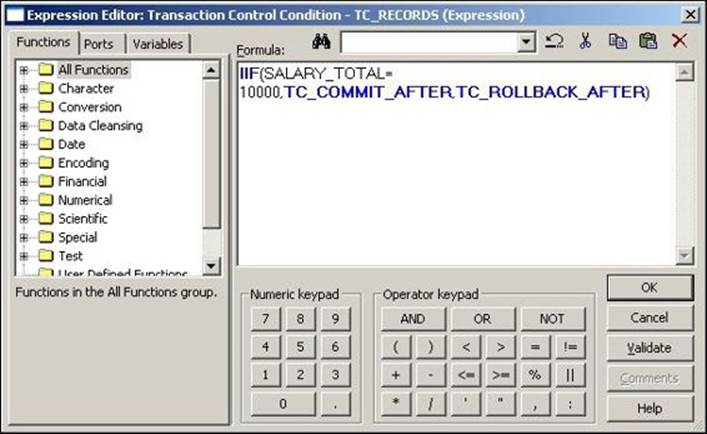
5. Finally, click on OK.

The mapping using the Transaction Control transformation is now complete.

The Transaction Control transformation supports the following built-in variables in the expression editor:

· TC_COMMIT_BEFORE: Integration Service commits the current record, starts processing a new record, and then writes the current row to the target.

· TC_COMMIT_AFTER: Integration Service commits and writes the current record to the target and then starts processing the new record.

· TC_ROLLBACK_BEFORE: Integration Service rolls back the current record, starts processing the new record, and then writes the current row to the target.

· TC_ROLLBACK_AFTER: Integration Service writes the current record to the target, rolls back the current record, and then starts processing the new record.

· TC_CONTINUE_TRANSACTION: This is the default value for the Transaction Control transformation. Integration Service does not perform any transaction operations for the record.

With this, we have seen the details related to Transaction Control transformations. It is not recommended that you use Transaction Control transformation in the mapping, as it hampers performance by checking each record for a commit or rollback. So the best way is to use the commit interval property in the session task.

Types of lookup cache

A cache is the temporary memory that is created when you execute the process. Caches are created automatically when the process starts and is deleted automatically once the process is complete. The amount of cache memory is decided based on the property you define at the transformation level or session level. You usually set the property as the default, so it can increase the size of the cache as required. If the size required to cache the data is more than the cache size defined, the process fails with an overflow error. There are different types of caches available.

Building the cache – sequential or concurrent

You can define the session property to create the cache either sequentially or concurrently.

Sequential cache

When you choose to create the cache sequentially, Integration Service caches the data in a row-wise manner as the records enter the Lookup transformation. When the first record enters the Lookup transformation, the lookup cache gets created and stores the matching record from the lookup table or file in the cache. This way, the cache stores only matching data. This helps save the cache space by not storing the unnecessary data.

Concurrent cache

When you choose to create caches concurrently, Integration Service does not wait for the data to flow from the source, but it first caches the complete data. Once the caching is complete, it allows the data to flow from the source. When you select concurrent cache, performance is better than sequential caches, as the scanning happens internally using the data stored in cache.

Persistent cache – the permanent one

You can configure caches to permanently save data. By default, caches are created as nonpersistent, that is, they will be deleted once the session run is complete. If the lookup table or file does not change across the session runs, you can use the existing persistent cache.

Suppose that you have a process that is scheduled to run every day and you are using a Lookup transformation to look up a reference table that is not supposed to change for 6 months. When you use a nonpersistent cache every day, the same data will be stored in cache. This will waste time and space every day. If you choose to create a persistent cache, Integration Service makes the cache permanent in the form of a file in the $PMCacheDir location, so you save the time required to create and delete the cache memory every day.

When the data in the lookup table changes, you need to rebuild the cache. You can define the condition in the session task to rebuild the cache by overwriting the existing cache. To rebuild the cache, you need to check the rebuild option in the session property, as discussed in the session properties in Chapter 5, Using the Workflow Manager Screen – Advanced.

Sharing cache – named or unnamed

You can enhance performance and save the cache memory by sharing the cache if there are multiple Lookup transformations used in a mapping. If you have the same structure for both the Lookup transformations, sharing the cache will help enhance performance by creating the cache only once. This way, we avoid creating the cache multiple times. You can share both named and unnamed caches.

Sharing unnamed cache

If you have multiple Lookup transformations used in a single mapping, you can share the unnamed cache. As the Lookup transformations are present in the same mapping, naming the cache is not mandatory. Integration Service creates the cache while processing the first record in the first Lookup transformation and shares the cache with other lookups in the mapping.

Sharing named cache

You can share the named cache with multiple Lookup transformations in the same mapping or in other mappings. As the cache is named, you can assign the same cache using the name in another mapping.

When you process the first mapping with a Lookup transformation, it saves the cache in the defined cache directory and with the defined cache filename. When you process the second mapping, it searches for the same location and cache file and uses the data. If Integration Service does not find the mentioned cache file, it creates the new cache.

If you simultaneously run multiple sessions that use the same cache file, Integration Service processes both the sessions successfully only if the Lookup transformation is configured for read-only from the cache. If there is a scenario where both the Lookup transformations are trying to update the cache file, or a scenario where one lookup is trying to read the cache file and the other is trying to update the cache, the session will fail as there is a conflict in the processing.

Sharing the cache helps enhance performance by utilizing the cache created. This way, we save the processing time and repository space by not storing the same data for Lookup transformations multiple times.

Modifying cache – static or dynamic

When you create a cache, you can configure it to be static or dynamic.

Static cache

A cache is said to be static if it does not change with the changes happening in the lookup table. A static cache is not synchronized with the lookup table.

By default, Integration Service creates a static cache. A lookup cache is created as soon as the first record enters the Lookup transformation. Integration Service does not update the cache while it is processing the data.

Dynamic cache

A cache is said to be dynamic if it changes with the changes happening in the lookup table. The dynamic cache is synchronized with the lookup table.

From the Lookup transformation properties, you can choose to make the cache dynamic. The lookup cache is created as soon as the first record enters the Lookup transformation. Integration Service keeps on updating the cache while it is processing the data. It marks the record INSERT for new rows inserted in dynamic cache. For the record that is updated, it marks the record as updated in the cache. For every record that doesn't change, Integration Service marks it as unchanged.

You use the dynamic cache while you process slowly changing dimension tables. For every record inserted into the target, the record will be inserted in the cache. For every record updated in the target, the record will be updated in the cache. A similar process happens for the deleted and rejected records.

Tracing levels

Tracing levels in Informatica define the amount of data you wish to write in the session log when you execute the workflow. The tracing level is a very important aspect of Informatica, as it helps in analyzing errors. It is also very helpful in finding the bugs in the process and you can define it in every transformation. The tracing level option is present in every transformation properties window. There are four types of tracing levels available:

· Normal: When you set the tracing level as Normal, Informatica stores the status information, information about errors, and information about skipped rows. You get detailed information but not at an individual row level.

· Terse: When you set the tracing level as Terse, Informatica stores the error information and the information of rejected records. Terse tracing level occupies less space than Normal.

· Verbose Initialization: When you set the tracing level as Verbose Initialize, it stores the process details related to the startup, details about index, data files created, and more details of the transformation process in addition to details stored in the normal tracing. This tracing level takes more space than Normal and Terse.

· Verbose Data: This is the most detailed level of tracing. It occupies more space and takes more time than the other three levels. It stores row-level data in the session log. It writes the truncation information whenever it truncates the data. It also writes the data to the error log if you enable row-error logging.

The default tracing level is Normal. You can change the tracing level to Terse in order to enhance performance. The tracing level can be defined at an individual transformation level, or you can override the tracing level by defining it at the session level.

Summary

We have discussed the most important aspect of the Informatica PowerCenter tool in this chapter. We also talked about most of the widely used transformations in this chapter. Other transformations that have intentionally not been discussed in this chapter are very rarely used. We have talked about the functions of various transformations. We learned about the usage of ports and expression editors in various transformations. We discussed the classification of the transformations: active/passive and connected/unconnected. We learned about the different types of caches and the different types of tracing levels available.

In the next chapter, we will discuss the fourth client screen, Repository Manager. We have seen the usage of other screens. We will see how the Repository Manager screen is used to deploy the code across the various environments in Informatica.