Machine Learning with R Cookbook (2015)
Chapter 1. Practical Machine Learning with R
In this chapter, we will cover the following topics:
· Downloading and installing R
· Downloading and installing RStudio
· Installing and loading packages
· Reading and writing data
· Using R to manipulate data
· Applying basic statistics
· Visualizing data
· Getting a dataset for machine learning
Introduction
The aim of machine learning is to uncover hidden patterns, unknown correlations, and find useful information from data. In addition to this, through incorporation with data analysis, machine learning can be used to perform predictive analysis. With machine learning, the analysis of business operations and processes is not limited to human scale thinking; machine scale analysis enables businesses to capture hidden values in big data.
Machine learning has similarities to the human reasoning process. Unlike traditional analysis, the generated model cannot evolve as data is accumulated. Machine learning can learn from the data that is processed and analyzed. In other words, the more data that is processed, the more it can learn.
R, as a dialect of GNU-S, is a powerful statistical language that can be used to manipulate and analyze data. Additionally, R provides many machine learning packages and visualization functions, which enable users to analyze data on the fly. Most importantly, R is open source and free.
Using R greatly simplifies machine learning. All you need to know is how each algorithm can solve your problem, and then you can simply use a written package to quickly generate prediction models on data with a few command lines. For example, you can either perform Naïve Bayes for spam mail filtering, conduct k-means clustering for customer segmentation, use linear regression to forecast house prices, or implement a hidden Markov model to predict the stock market, as shown in the following screenshot:

Stock market prediction using R
Moreover, you can perform nonlinear dimension reduction to calculate the dissimilarity of image data, and visualize the clustered graph, as shown in the following screenshot. All you need to do is follow the recipes provided in this book.
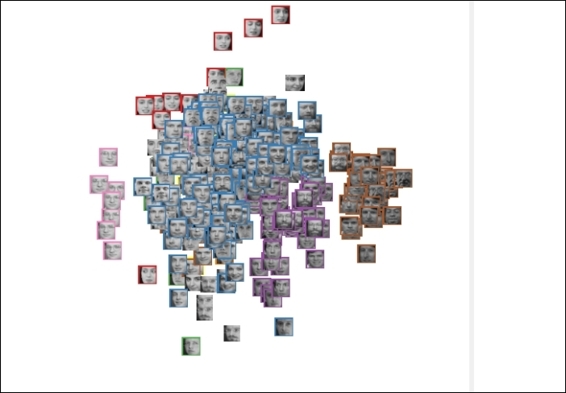
A clustered graph of face image data
This chapter serves as an overall introduction to machine learning and R; the first few recipes introduce how to set up the R environment and integrated development environment, RStudio. After setting up the environment, the following recipe introduces package installation and loading. In order to understand how data analysis is practiced using R, the next four recipes cover data read/write, data manipulation, basic statistics, and data visualization using R. The last recipe in the chapter lists useful data sources and resources.
Downloading and installing R
To use R, you must first install it on your computer. This recipe gives detailed instructions on how to download and install R.
Getting ready
If you are new to the R language, you can find a detailed introduction, language history, and functionality on the official website (http://www.r-project.org/). When you are ready to download and install R, please access the following link: http://cran.r-project.org/.
How to do it...
Please perform the following steps to download and install R for Windows and Mac users:
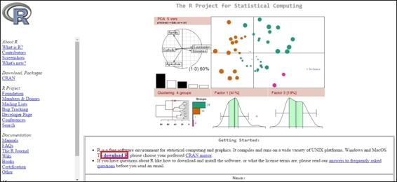
1. Go to the R CRAN website, http://www.r-project.org/, and click on the download R link, that is, http://cran.r-project.org/mirrors.html):
2. You may select the mirror location closest to you:
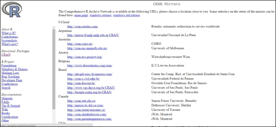
CRAN mirrors
3. Select the correct download link based on your operating system:
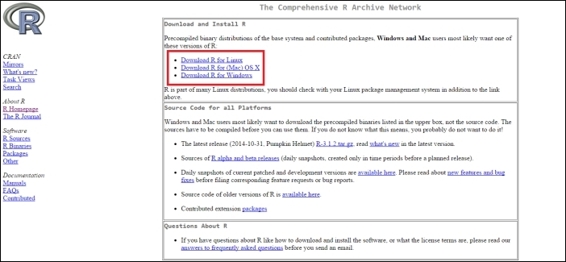
Click on the download link based on your OS
As the installation of R differs for Windows and Mac, the steps required to install R for each OS are provided here.
For Windows users:
1. Click on Download R for Windows, as shown in the following screenshot, and then click on base:
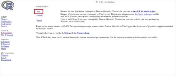
Go to "Download R for Windows" and click "base"
2. Click on Download R 3.x.x for Windows:
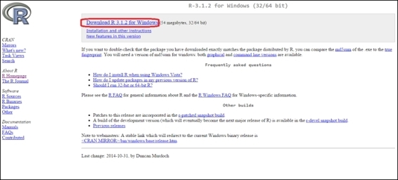
Click "Download R 3.x.x for Windows"
3. The installation file should be downloaded. Once the download is finished, you can double-click on the installation file and begin installing R:
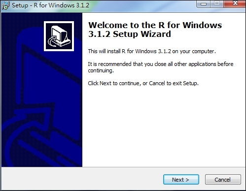
4. The Windows installation of R is quite straightforward; the installation GUI may instruct you on how to install the program step by step (public license, destination location, select components, startup options, startup menu folder, and select additional tasks). Leave all the installation options as the default settings if you do not want to make any changes.
5. After successfully completing the installation, a shortcut to the R application will appear in your Start menu, which will open the R Console:

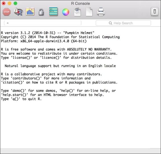
The Windows R Console
For Mac OS X users:
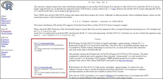
1. Go to Download R for (Mac) OS X, as shown in this screenshot.
2. Click on the latest version (.pkg file extension) according to your Mac OS version:
3. Double-click on the downloaded installation file (.pkg extension) and begin to install R. Leave all the installation options as the default settings if you do not want to make any changes:
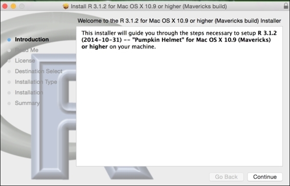
4. Follow the onscreen instructions, Introduction, Read Me, License, Destination Select, Installation Type, Installation, Summary, and click on continue to complete the installation.
5. After the file is installed, you can use Spotlight Search or go to the application folder to find R:
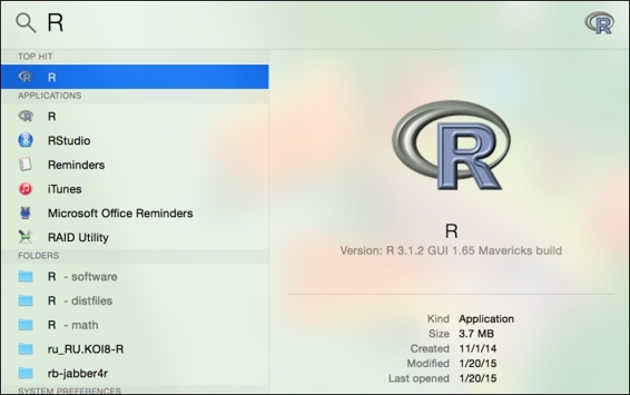
Use "Spotlight Search" to find R
6. Click on R to open R Console:
As an alternative to downloading a Mac .pkg file to install R, Mac users can also install R using Homebrew:
1. Download XQuartz-2.X.X.dmg from https://xquartz.macosforge.org/landing/.
2. Double-click on the .dmg file to mount it.
3. Update brew with the following command line:
4. $ brew update
4. Clone the repository and symlink all its formulae to homebrew/science:
5. $ brew tap homebrew/science
5. Install gfortran:
6. $ brew install gfortran
6. Install R:
7. $ brew install R
For Linux users, there are precompiled binaries for Debian, Red Hat, SUSE, and Ubuntu. Alternatively, you can install R from a source code. Besides downloading precompiled binaries, you can install R for Linux through a package manager. Here are the installation steps for CentOS and Ubuntu.
Downloading and installing R on Ubuntu:
1. Add the entry to the /etc/apt/sources.list file:
2. $ sudo sh -c "echo 'deb http:// cran.stat.ucla.edu/bin/linux/ubuntu precise/' >> /etc/apt/sources.list"
2. Then, update the repository:
3. $ sudo apt-get update
3. Install R with the following command:
4. $ sudo apt-get install r-base
4. Start R in the command line:
5. $ R
Downloading and installing R on CentOS 5:
1. Get rpm CentOS5 RHEL EPEL repository of CentOS5:
2. $ wget http://dl.fedoraproject.org/pub/epel/5/x86_64/epel-release-5-4.noarch.rpm
2. Install CentOS5 RHEL EPEL repository:
3. $ sudo rpm -Uvh epel-release-5-4.noarch.rpm
3. Update the installed packages:
4. $ sudo yum update
4. Install R through the repository:
5. $ sudo yum install R
5. Start R in the command line:
6. $ R
Downloading and installing R on CentOS 6:
1. Get rpm CentOS5 RHEL EPEL repository of CentOS6:
2. $ wget http://dl.fedoraproject.org/pub/epel/6/x86_64/epel-release-6-8.noarch.rpm
2. Install the CentOS5 RHEL EPEL repository:
3. $ sudo rpm -Uvh epel-release-6-8.noarch.rpm
3. Update the installed packages:
4. $ sudo yum update
4. Install R through the repository:
5. $ sudo yum install R
5. Start R in the command line:
6. $ R
How it works...
CRAN provides precompiled binaries for Linux, Mac OS X, and Windows. For Mac and Windows users, the installation procedures are straightforward. You can generally follow onscreen instructions to complete the installation. For Linux users, you can use the package manager provided for each platform to install R or build R from the source code.
See also
· For those planning to build R from the source code, refer to R Installation and Administration (http://cran.r-project.org/doc/manuals/R-admin.html), which illustrates how to install R on a variety of platforms.
Downloading and installing RStudio
To write an R script, one can use R Console, R commander, or any text editor (EMACS, VIM, or sublime). However, the assistance of RStudio, an integrated development environment (IDE) for R, can make development a lot easier.
RStudio provides comprehensive facilities for software development. Built-in features such as syntax highlighting, code completion, and smart indentation help maximize productivity. To make R programming more manageable, RStudio also integrates the main interface into a four-panel layout. It includes an interactive R Console, a tabbed source code editor, a panel for the currently active objects/history, and a tabbed panel for the file browser/plot window/package install window/R help window. Moreover, RStudio is open source and is available for many platforms, such as Windows, Mac OS X, and Linux. This recipe shows how to download and install RStudio.
Getting ready
RStudio requires a working R installation; when RStudio loads, it must be able to locate a version of R. You must therefore have completed the previous recipe with R installed on your OS before proceeding to install RStudio.
How to do it...
Perform the following steps to download and install RStudio for Windows and Mac users:
1. Access RStudio's official site by using the following URL: http://www.rstudio.com/products/RStudio/.
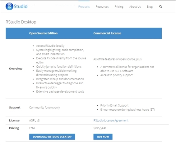
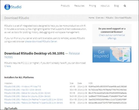
2. For a desktop version installation, click on Download RStudio Desktop (http://www.rstudio.com/products/rstudio/download/) and choose the RStudio recommended for your system. Download the relevant packages:
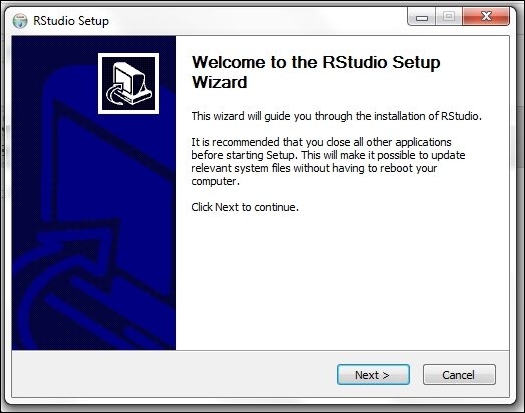
3. Install RStudio by double-clicking on the downloaded packages. For Windows users, follow the onscreen instruction to install the application:
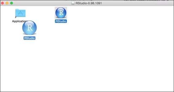
4. For Mac users, simply drag the RStudio icon to the Applications folder:
5. Start RStudio:
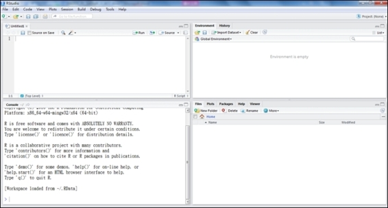
The RStudio console
Perform the following steps for downloading and installing RStudio for Ubuntu/Debian and RedHat/Centos users:
For Debian(6+)/Ubuntu(10.04+) 32-bit:
$ wget http://download1.rstudio.org/rstudio-0.98.1091-i386.deb
$ sudo gdebi rstudio-0.98. 1091-i386.deb
For Debian(6+)/Ubuntu(10.04+) 64-bit:
$ wget http://download1.rstudio.org/rstudio-0.98. 1091-amd64.deb
$ sudo gdebi rstudio-0.98. 1091-amd64.deb
For RedHat/CentOS(5,4+) 32 bit:
$ wget http://download1.rstudio.org/rstudio-0.98. 1091-i686.rpm
$ sudo yum install --nogpgcheck rstudio-0.98. 1091-i686.rpm
For RedHat/CentOS(5,4+) 64 bit:
$ wget http://download1.rstudio.org/rstudio-0.98. 1091-x86_64.rpm
$ sudo yum install --nogpgcheck rstudio-0.98. 1091-x86_64.rpm
How it works
The RStudio program can be run on the desktop or through a web browser. The desktop version is available for Windows, Mac OS X, and Linux platforms with similar operations across all platforms. For Windows and Mac users, after downloading the precompiled package of RStudio, follow the onscreen instructions, shown in the preceding steps, to complete the installation. Linux users may use the package management system provided for installation.
See also
· In addition to the desktop version, users may install a server version to provide access to multiple users. The server version provides a URL that users can access to use the RStudio resources. To install RStudio, please refer to the following link: http://www.rstudio.com/ide/download/server.html. This page provides installation instructions for the following Linux distributions: Debian (6+), Ubuntu (10.04+), RedHat, and CentOS (5.4+).
· For other Linux distributions, you can build RStudio from the source code.
Installing and loading packages
After successfully installing R, users can download, install, and update packages from the repositories. As R allows users to create their own packages, official and non-official repositories are provided to manage these user-created packages. CRAN is the official R package repository. Currently, the CRAN package repository features 6,379 available packages (as of 02/27/2015). Through the use of the packages provided on CRAN, users may extend the functionality of R to machine learning, statistics, and related purposes. CRAN is a network of FTP and web servers around the world that store identical, up-to-date versions of code and documentation for R. You may select the closest CRAN mirror to your location to download packages.
Getting ready
Start an R session on your host computer.
How to do it...
Perform the following steps to install and load R packages:
1. To load a list of installed packages:
2. > library()
2. Setting the default CRAN mirror:
3. > chooseCRANmirror()
R will return a list of CRAN mirrors, and then ask the user to either type a mirror ID to select it, or enter zero to exit:
1. Install a package from CRAN; take package e1071 as an example:
2. > install.packages("e1071")
2. Update a package from CRAN; take package e1071 as an example:
3. > update.packages("e1071")
3. Load the package the package:
4. > library(e1071)
4. If you would like to view the documentation of the package, you can use the help function:
5. > help(package ="e1071")
5. If you would like to view the documentation of the function, you can use the help function:
6. > help(svm, e1071)
6. Alternatively, you can use the help shortcut, ?, to view the help document for this function:
7. > ?e1071::svm
7. If the function does not provide any documentation, you may want to search the supplied documentation for a given keyword. For example, if you wish to search for documentation related to svm:
8. > help.search("svm")
8. Alternatively, you can use ?? as the shortcut for help.search:
9. > ??svm
9. To view the argument taken for the function, simply use the args function. For example, if you would like to know the argument taken for the lm function:
10.> args(lm)
10.Some packages will provide examples and demos; you can use example or demo to view an example or demo. For example, one can view an example of the lm package and a demo of the graphics package by typing the following commands:
11.> example(lm)
12.> demo(graphics)
11.To view all the available demos, you may use the demo function to list all of them:
12.> demo()
How it works
This recipe first introduces how to view loaded packages, install packages from CRAN, and load new packages. Before installing packages, those of you who are interested in the listing of the CRAN package can refer to http://cran.r-project.org/web/packages/available_packages_by_name.html.
When a package is installed, documentation related to the package is also provided. You are, therefore, able to view the documentation or the related help pages of installed packages and functions. Additionally, demos and examples are provided by packages that can help users understand the capability of the installed package.
See also
· Besides installing packages from CRAN, there are other R package repositories, including Crantastic, a community site for rating and reviewing CRAN packages, and R-Forge, a central platform for the collaborative development of R packages. In addition to this, Bioconductor provides R packages for the analysis of genomic data.
· If you would like to find relevant functions and packages, please visit the list of task views at http://cran.r-project.org/web/views/, or search for keywords at http://rseek.org.
Reading and writing data
Before starting to explore data, you must load the data into the R session. This recipe will introduce methods to load data either from a file into the memory or use the predefined data within R.
Getting ready
First, start an R session on your machine. As this recipe involves steps toward the file IO, if the user does not specify the full path, read and write activity will take place in the current working directory.
You can simply type getwd() in the R session to obtain the current working directory location. However, if you would like to change the current working directory, you can use setwd("<path>"), where <path> can be replaced as your desired path, to specify the working directory.
How to do it...
Perform the following steps to read and write data with R:
1. To view the built-in datasets of R, type the following command:
2. > data()
2. R will return a list of datasets in a dataset package, and the list comprises the name and description of each dataset.
3. To load the dataset iris into an R session, type the following command:
4. > data(iris)
4. The dataset iris is now loaded into the data frame format, which is a common data structure in R to store a data table.
5. To view the data type of iris, simply use the class function:
6. > class(iris)
7. [1] "data.frame"
6. The data.frame console print shows that the iris dataset is in the structure of data frame.
7. Use the save function to store an object in a file. For example, to save the loaded iris data into myData.RData, use the following command:
8. > save(iris, file="myData.RData")
8. Use the load function to read a saved object into an R session. For example, to load iris data from myData.RData, use the following command:
9. > load("myData.RData")
9. In addition to using built-in datasets, R also provides a function to import data from text into a data frame. For example, the read.table function can format a given text into a data frame:
10.> test.data = read.table(header = TRUE, text = "
11.+ a b
12.+ 1 2
13.+ 3 4
14.+ ")
10.You can also use row.names and col.names to specify the names of columns and rows:
11.> test.data = read.table(text = "
12.+ 1 2
13.+ 3 4",
14.+ col.names=c("a","b"),
15.+ row.names = c("first","second"))
11.View the class of the test.data variable:
12.> class(test.data)
13.[1] "data.frame"
12.The class function shows that the test.data variable contains a data frame.
13.In addition to importing data by using the read.table function, you can use the write.table function to export data to a text file:
14.> write.table(test.data, file = "test.txt" , sep = " ")
14.The write.table function will write the content of test.data into test.txt (the written path can be found by typing getwd()), with a separation delimiter as white space.
15.Similar to write.table, write.csv can also export data to a file. However, write.csv uses a comma as the default delimiter:
16.> write.csv(test.data, file = "test.csv")
16.With the read.csv function, the csv file can be imported as a data frame. However, the last example writes column and row names of the data frame to the test.csv file. Therefore, specifying header to TRUE and row names as the first column within the function can ensure the read data frame will not treat the header and the first column as values:
17.> csv.data = read.csv("test.csv", header = TRUE, row.names=1)
18.> head(csv.data)
19. a b
20.1 1 2
21.2 3 4
How it works
Generally, data for collection may be in multiple files and different formats. To exchange data between files and RData, R provides many built-in functions, such as save, load, read.csv, read.table, write.csv, and write.table.
This example first demonstrates how to load the built-in dataset iris into an R session. The iris dataset is the most famous and commonly used dataset in the field of machine learning. Here, we use the iris dataset as an example. The recipe shows how to save RData and load it with the save and load functions. Furthermore, the example explains how to use read.table, write.table, read.csv, and write.csv to exchange data from files to a data frame. The use of the R IO function to read and write data is very important as most of the data sources are external. Therefore, you have to use these functions to load data into an R session.
See also
For the load, read.table, and read.csv functions, the file to be read can also be a complete URL (for supported URLs, use ?url for more information).
On some occasions, data may be in an Excel file instead of a flat text file. The WriteXLS package allows writing an object into an Excel file with a given variable in the first argument and the file to be written in the second argument:
1. Install the WriteXLS package:
2. > install.packages("WriteXLS")
2. Load the WriteXLS package:
3. > library("WriteXLS")
3. Use the WriteXLS function to write the data frame iris into a file named iris.xls:
4. > WriteXLS("iris", ExcelFileName="iris.xls")
Using R to manipulate data
This recipe will discuss how to use the built-in R functions to manipulate data. As data manipulation is the most time consuming part of most analysis procedures, you should gain knowledge of how to apply these functions on data.
Getting ready
Ensure you have completed the previous recipes by installing R on your operating system.
How to do it...
Perform the following steps to manipulate the data with R.
Subset the data using the bracelet notation:
1. Load the dataset iris into the R session:
2. > data(iris)
2. To select values, you may use a bracket notation that designates the indices of the dataset. The first index is for the rows and the second for the columns:
3. > iris[1,"Sepal.Length"]
4. [1] 5.1
3. You can also select multiple columns using c():
4. > Sepal.iris = iris[, c("Sepal.Length", "Sepal.Width")]
4. You can then use str() to summarize and display the internal structure of Sepal.iris:
5. > str(Sepal.iris)
6. 'data.frame': 150 obs. of 2 variables:
7. $ Sepal.Length: num 5.1 4.9 4.7 4.6 5 5.4 4.6 5 4.4 4.9 ...
8. $ Sepal.Width : num 3.5 3 3.2 3.1 3.6 3.9 3.4 3.4 2.9 3.1 ..
5. To subset data with the rows of given indices, you can specify the indices at the first index with the bracket notation. In this example, we show you how to subset data with the top five records with the Sepal.Length column and the Sepal.Width selected:
6. > Five.Sepal.iris = iris[1:5, c("Sepal.Length", "Sepal.Width")]
7. > str(Five.Sepal.iris)
8. 'data.frame': 5 obs. of 2 variables:
9. $ Sepal.Length: num 5.1 4.9 4.7 4.6 5
10. $ Sepal.Width : num 3.5 3 3.2 3.1 3.6
6. It is also possible to set conditions to filter the data. For example, to filter returned records containing the setosa data with all five variables. In the following example, the first index specifies the returning criteria, and the second index specifies the range of indices of the variable returned:
7. > setosa.data = iris[iris$Species=="setosa",1:5]
8. > str(setosa.data)
9. 'data.frame': 50 obs. of 5 variables:
10. $ Sepal.Length: num 5.1 4.9 4.7 4.6 5 5.4 4.6 5 4.4 4.9 ...
11. $ Sepal.Width : num 3.5 3 3.2 3.1 3.6 3.9 3.4 3.4 2.9 3.1 ...
12. $ Petal.Length: num 1.4 1.4 1.3 1.5 1.4 1.7 1.4 1.5 1.4 1.5 ...
13. $ Petal.Width : num 0.2 0.2 0.2 0.2 0.2 0.4 0.3 0.2 0.2 0.1 ...
14. $ Species : Factor w/ 3 levels "setosa","versicolor",..: 1 1 1 1 1 1 1 1 1 1 ...
7. Alternatively, the which function returns the indexes of satisfied data. The following example returns indices of the iris data containing species equal to setosa:
8. > which(iris$Species=="setosa")
9. [1] 1 2 3 4 5 6 7 8 9 10 11 12 13 14 15 16 17 18
10.[19] 19 20 21 22 23 24 25 26 27 28 29 30 31 32 33 34 35 36
11.[37] 37 38 39 40 41 42 43 44 45 46 47 48 49 50
8. The indices returned by the operation can then be applied as the index to select the iris containing the setosa species. The following example returns the setosa with all five variables:
9. > setosa.data = iris[which(iris$Species=="setosa"),1:5]
10.> str(setosa.data)
11.'data.frame': 50 obs. of 5 variables:
12. $ Sepal.Length: num 5.1 4.9 4.7 4.6 5 5.4 4.6 5 4.4 4.9 ...
13. $ Sepal.Width : num 3.5 3 3.2 3.1 3.6 3.9 3.4 3.4 2.9 3.1 ...
14. $ Petal.Length: num 1.4 1.4 1.3 1.5 1.4 1.7 1.4 1.5 1.4 1.5 ...
15. $ Petal.Width : num 0.2 0.2 0.2 0.2 0.2 0.4 0.3 0.2 0.2 0.1 ...
16. $ Species : Factor w/ 3 levels "setosa","versicolor",..: 1 1 1 1 1 1 1 1 1 1 ...
Subset data using the subset function:
1. Besides using the bracket notation, R provides a subset function that enables users to subset the data frame by observations with a logical statement.
2. First, subset species, sepal length, and sepal width out of the iris data. To select the sepal length and width out of the iris data, one should specify the column to be subset in the select argument:
3. > Sepal.data = subset(iris, select=c("Sepal.Length", "Sepal.Width"))
4. > str(Sepal.data)
5. 'data.frame': 150 obs. of 2 variables:
6. $ Sepal.Length: num 5.1 4.9 4.7 4.6 5 5.4 4.6 5 4.4 4.9 ...
7. $ Sepal.Width : num 3.5 3 3.2 3.1 3.6 3.9 3.4 3.4 2.9 3.1 ...
This reveals that Sepal.data contains 150 objects with the Sepal.Length variable and Sepal.Width.
1. On the other hand, you can use a subset argument to get subset data containing setosa only. In the second argument of the subset function, you can specify the subset criteria:
2. > setosa.data = subset(iris, Species =="setosa")
3. > str(setosa.data)
4. 'data.frame': 50 obs. of 5 variables:
5. $ Sepal.Length: num 5.1 4.9 4.7 4.6 5 5.4 4.6 5 4.4 4.9 ...
6. $ Sepal.Width : num 3.5 3 3.2 3.1 3.6 3.9 3.4 3.4 2.9 3.1 ...
7. $ Petal.Length: num 1.4 1.4 1.3 1.5 1.4 1.7 1.4 1.5 1.4 1.5 ...
8. $ Petal.Width : num 0.2 0.2 0.2 0.2 0.2 0.4 0.3 0.2 0.2 0.1 ...
9. $ Species : Factor w/ 3 levels "setosa","versicolor",..: 1 1 1 1 1 1 1 1 1 1 ...
2. Most of the time, you may want to apply a union or intersect a condition while subsetting data. The OR and AND operations can be further employed for this purpose. For example, if you would like to retrieve data with Petal.Width >=0.2 and Petal.Length < = 1.4:
3. > example.data= subset(iris, Petal.Length <=1.4 & Petal.Width >= 0.2, select=Species )
4. > str(example.data)
5. 'data.frame': 21 obs. of 1 variable:
6. $ Species: Factor w/ 3 levels "setosa","versicolor",..: 1 1 1 1 1 1 1 1 1 1 ...
Merging data: merging data involves joining two data frames into a merged data frame by a common column or row name. The following example shows how to merge the flower.type data frame and the first three rows of the iris with a common row name within the Species column:
> flower.type = data.frame(Species = "setosa", Flower = "iris")
> merge(flower.type, iris[1:3,], by ="Species")
Species Flower Sepal.Length Sepal.Width Petal.Length Petal.Width
1 setosa iris 5.1 3.5 1.4 0.2
2 setosa iris 4.9 3.0 1.4 0.2
3 setosa iris 4.7 3.2 1.3 0.2
Ordering data: the order function will return the index of a sorted data frame with a specified column. The following example shows the results from the first six records with the sepal length ordered (from big to small) iris data
> head(iris[order(iris$Sepal.Length, decreasing = TRUE),])
Sepal.Length Sepal.Width Petal.Length Petal.Width Species
132 7.9 3.8 6.4 2.0 virginica
118 7.7 3.8 6.7 2.2 virginica
119 7.7 2.6 6.9 2.3 virginica
123 7.7 2.8 6.7 2.0 virginica
136 7.7 3.0 6.1 2.3 virginica
106 7.6 3.0 6.6 2.1 virginica
How it works
Before conducting data analysis, it is important to organize collected data into a structured format. Therefore, we can simply use the R data frame to subset, merge, and order a dataset. This recipe first introduces two methods to subset data: one uses the bracket notation, while the other uses the subset function. You can use both methods to generate the subset data by selecting columns and filtering data with the given criteria. The recipe then introduces the merge function to merge data frames. Last, the recipe introduces how to use order to sort the data.
There's more...
The sub and gsub functions allow using regular expression to substitute a string. The sub and gsub functions perform the replacement of the first and all the other matches, respectively:
> sub("e", "q", names(iris))
[1] "Sqpal.Length" "Sqpal.Width" "Pqtal.Length" "Pqtal.Width" "Spqcies"
> gsub("e", "q", names(iris))
[1] "Sqpal.Lqngth" "Sqpal.Width" "Pqtal.Lqngth" "Pqtal.Width" "Spqciqs"
Applying basic statistics
R provides a wide range of statistical functions, allowing users to obtain the summary statistics of data, generate frequency and contingency tables, produce correlations, and conduct statistical inferences. This recipe covers basic statistics that can be applied to a dataset.
Getting ready
Ensure you have completed the previous recipes by installing R on your operating system.
How to do it...
Perform the following steps to apply statistics on a dataset:
1. Load the iris data into an R session:
2. > data(iris)
2. Observe the format of the data:
3. > class(iris)
4. [1] "data.frame"
3. The iris dataset is a data frame containing four numeric attributes: petal length, petal width, sepal width, and sepal length. For numeric values, you can perform descriptive statistics, such as mean, sd, var, min, max, median, range, and quantile. These can be applied to any of the four attributes in the dataset:
4. > mean(iris$Sepal.Length)
5. [1] 5.843333
6. > sd(iris$Sepal.Length)
7. [1] 0.8280661
8. > var(iris$Sepal.Length)
9. [1] 0.6856935
10.> min(iris$Sepal.Length)
11.[1] 4.3
12.> max(iris$Sepal.Length)
13.[1] 7.9
14.> median(iris$Sepal.Length)
15.[1] 5.8
16.> range(iris$Sepal.Length)
17.[1] 4.3 7.9
18.> quantile(iris$Sepal.Length)
19. 0% 25% 50% 75% 100%
20. 4.3 5.1 5.8 6.4 7.9
4. The preceding example demonstrates how to apply descriptive statistics on a single variable. In order to obtain summary statistics on every numeric attribute of the data frame, one may use sapply. For example, to apply the mean on the first four attributes in the iris data frame, ignore the na value by setting na.rm as TRUE:
5. > sapply(iris[1:4], mean, na.rm=TRUE)
6. Sepal.Length Sepal.Width Petal.Length Petal.Width
7. 5.843333 3.057333 3.758000 1.199333
5. As an alternative to using sapply to apply descriptive statistics on given attributes, R offers the summary function that provides a full range of descriptive statistics. In the following example, the summary function provides the mean, median, 25th and 75th quartiles, min, and max of every iris dataset numeric attribute:
6. > summary(iris)
7. Sepal.Length Sepal.Width Petal.Length Petal.Width Species
8. Min. :4.300 Min. :2.000 Min. :1.000 Min. :0.100 setosa :50
9. 1st Qu.:5.100 1st Qu.:2.800 1st Qu.:1.600 1st Qu.:0.300 versicolor:50
10. Median :5.800 Median :3.000 Median :4.350 Median :1.300 virginica :50
11. Mean :5.843 Mean :3.057 Mean :3.758 Mean :1.199
12. 3rd Qu.:6.400 3rd Qu.:3.300 3rd Qu.:5.100 3rd Qu.:1.800
13. Max. :7.900 Max. :4.400 Max. :6.900 Max. :2.500
6. The preceding example shows how to output the descriptive statistics of a single variable. R also provides the correlation for users to investigate the relationship between variables. The following example generates a 4x4 matrix by computing the correlation of each attribute pair within the iris:
7. > cor(iris[,1:4])
8. Sepal.Length Sepal.Width Petal.Length Petal.Width
9. Sepal.Length 1.0000000 -0.1175698 0.8717538 0.8179411
10.Sepal.Width -0.1175698 1.0000000 -0.4284401 -0.3661259
11.Petal.Length 0.8717538 -0.4284401 1.0000000 0.9628654
12.Petal.Width 0.8179411 -0.3661259 0.9628654 1.0000000
7. R also provides a function to compute the covariance of each attribute pair within the iris:
8. > cov(iris[,1:4])
9. Sepal.Length Sepal.Width Petal.Length Petal.Width
10.Sepal.Length 0.6856935 -0.0424340 1.2743154 0.5162707
11.Sepal.Width -0.0424340 0.1899794 -0.3296564 -0.1216394
12.Petal.Length 1.2743154 -0.3296564 3.1162779 1.2956094
13.Petal.Width 0.5162707 -0.1216394 1.2956094 0.5810063
8. Statistical tests are performed to access the significance of the results; here we demonstrate how to use a t-test to determine the statistical differences between two samples. In this example, we perform a t.test on the petal width an of an iris in either the setosa or versicolor species. If we obtain a p-value less than 0.5, we can be certain that the petal width between the setosa and versicolor will vary significantly:
9. > t.test(iris$Petal.Width[iris$Species=="setosa"],
10.+ iris$Petal.Width[iris$Species=="versicolor"])
11.
12. Welch Two Sample t-test
13.
14.data: iris$Petal.Width[iris$Species == "setosa"] and iris$Petal.Width[iris$Species == "versicolor"]
15.t = -34.0803, df = 74.755, p-value < 2.2e-16
16.alternative hypothesis: true difference in means is not equal to 0
17.95 percent confidence interval:
18. -1.143133 -1.016867
19.sample estimates:
20.mean of x mean of y
21. 0.246 1.326
9. Alternatively, you can perform a correlation test on the sepal length to the sepal width of an iris, and then retrieve a correlation score between the two variables. The stronger the positive correlation, the closer the value is to 1. The stronger the negative correlation, the closer the value is to -1:
10.> cor.test(iris$Sepal.Length, iris$Sepal.Width)
11.
12. Pearson's product-moment correlation
13.
14.data: iris$Sepal.Length and iris$Sepal.Width
15.t = -1.4403, df = 148, p-value = 0.1519
16.alternative hypothesis: true correlation is not equal to 0
17.95 percent confidence interval:
18. -0.27269325 0.04351158
19.sample estimates:
20. cor
21.-0.1175698
How it works...
R has a built-in statistics function, which enables the user to perform descriptive statistics on a single variable. The recipe first introduces how to apply mean, sd, var, min, max, median, range, and quantile on a single variable. Moreover, in order to apply the statistics on all four numeric variables, one can use the sapply function. In order to determine the relationships between multiple variables, one can conduct correlation and covariance. Finally, the recipe shows how to determine the statistical differences of two given samples by performing a statistical test.
There's more...
If you need to compute an aggregated summary statistics against data in different groups, you can use the aggregate and reshape functions to compute the summary statistics of data subsets:
1. Use aggregate to calculate the mean of each iris attribute group by the species:
2. > aggregate(x=iris[,1:4],by=list(iris$Species),FUN=mean)
2. Use reshape to calculate the mean of each iris attribute group by the species:
3. > library(reshape)
4. > iris.melt <- melt(iris,id='Species')
5. > cast(Species~variable,data=iris.melt,mean,
6. subset=Species %in% c('setosa','versicolor'),
7. margins='grand_row')
For information on reshape and aggregate, refer to the help documents by using ?reshape or ?aggregate.
Visualizing data
Visualization is a powerful way to communicate information through graphical means. Visual presentations make data easier to comprehend. This recipe presents some basic functions to plot charts, and demonstrates how visualizations are helpful in data exploration.
Getting ready
Ensure that you have completed the previous recipes by installing R on your operating system.
How to do it...
Perform the following steps to visualize a dataset:
1. Load the iris data into the R session:
2. > data(iris)
2. Calculate the frequency of species within the iris using the table command:
3. > table.iris = table(iris$Species)
4. > table.iris
5.
6. setosa versicolor virginica
7. 50 50 50
3. As the frequency in the table shows, each species represents 1/3 of the iris data. We can draw a simple pie chart to represent the distribution of species within the iris:
4. > pie(table.iris)
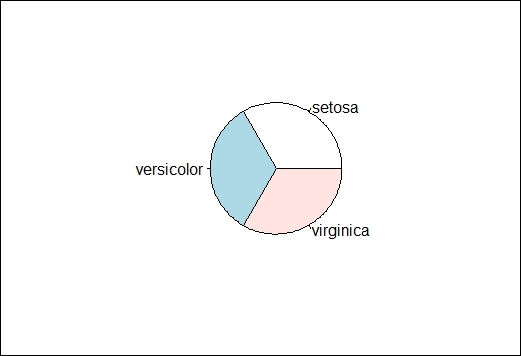
The pie chart of species distribution
4. The histogram creates a frequency plot of sorts along the x-axis. The following example produces a histogram of the sepal length:
5. > hist(iris$Sepal.Length)
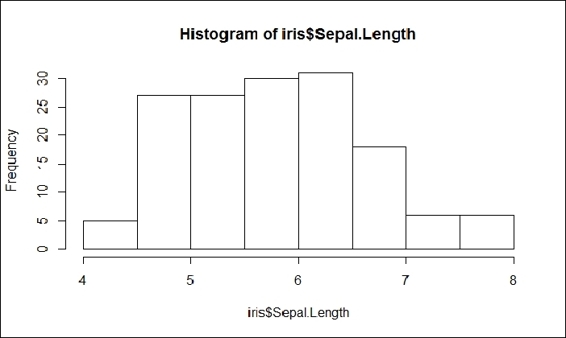
The histogram of the sepal length
5. In the histogram, the x-axis presents the sepal length and the y-axis presents the count for different sepal lengths. The histogram shows that for most irises, sepal lengths range from 4 cm to 8 cm.
6. Boxplots, also named box and whisker graphs, allow you to convey a lot of information in one simple plot. In such a graph, the line represents the median of the sample. The box itself shows the upper and lower quartiles. The whiskers show the range:
7. > boxplot(Petal.Width ~ Species, data = iris)
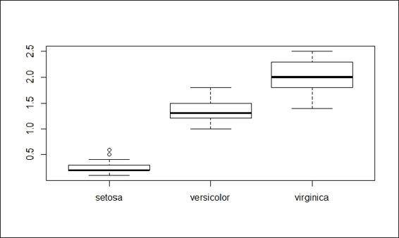
The boxplot of the petal width
7. The preceding screenshot clearly shows the median and upper range of the petal width of the setosa is much shorter than versicolor and virginica. Therefore, the petal width can be used as a substantial attribute to distinguish iris species.
8. A scatter plot is used when there are two variables to plot against one another. This example plots the petal length against the petal width and color dots in accordance to the species it belongs to:
9. > plot(x=iris$Petal.Length, y=iris$Petal.Width, col=iris$Species)
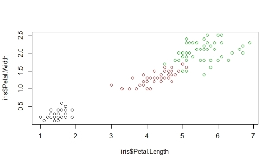
The scatter plot of the sepal length
9. The preceding screenshot is a scatter plot of the petal length against the petal width. As there are four attributes within the iris dataset, it takes six operations to plot all combinations. However, R provides a function named pairs, which can generate each subplot in one figure:
10.> pairs(iris[1:4], main = "Edgar Anderson's Iris Data", pch = 21, bg = c("red", "green3", "blue")[unclass(iris$Species)])
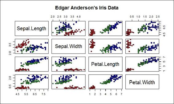
Pairs scatterplot of iris data
How it works...
R provides many built-in plot functions, which enable users to visualize data with different kinds of plots. This recipe demonstrates the use of pie charts that can present category distribution. A pie chart of an equal size shows that the number of each species is equal. A histogram plots the frequency of different sepal lengths. A box plot can convey a great deal of descriptive statistics, and shows that the petal width can be used to distinguish an iris species. Lastly, we introduced scatter plots, which plot variables on a single plot. In order to quickly generate a scatter plot containing all the pairs of iris data, one may use the pairs command.
See also
· ggplot2 is another plotting system for R, based on the implementation of Leland Wilkinson's grammar of graphics. It allows users to add, remove, or alter components in a plot with a higher abstraction. However, the level of abstraction results is slow compared to lattice graphics. For those of you interested in the topic of ggplot, you can refer to this site: http://ggplot2.org/.
Getting a dataset for machine learning
While R has a built-in dataset, the sample size and field of application is limited. Apart from generating data within a simulation, another approach is to obtain data from external data repositories. A famous data repository is the UCI machine learning repository, which contains both artificial and real datasets. This recipe introduces how to get a sample dataset from the UCI machine learning repository.
Getting ready
Ensure that you have completed the previous recipes by installing R on your operating system.
How to do it...
Perform the following steps to retrieve data for machine learning:
1. Access the UCI machine learning repository: http://archive.ics.uci.edu/ml/.
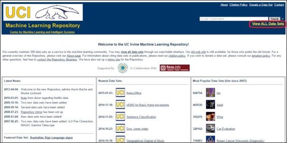
UCI data repository
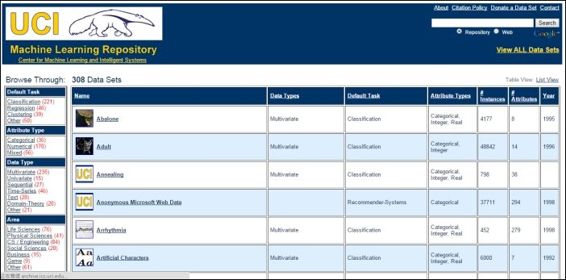
2. Click on View ALL Data Sets. Here you will find a list of datasets containing field names, such as Name, Data Types, Default Task, Attribute Types, # Instances, # Attributes, and Year:
3. Use Ctrl + F to search for Iris:
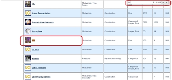
4. Click on Iris. This will display the data folder and the dataset description:
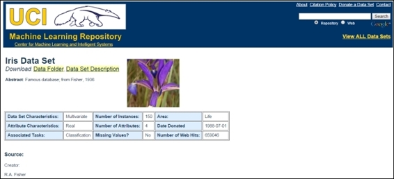
5. Click on Data Folder, which will display a directory containing the iris dataset:
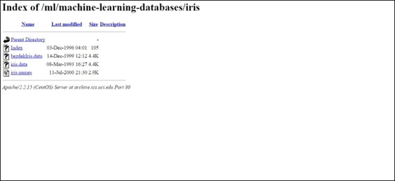
6. You can then either download iris.data or use the read.csv function to read the dataset:
7. > iris.data = read.csv(url("http://archive.ics.uci.edu/ml/machine-learning-databases/iris/iris.data"), header = FALSE, col.names = c("Sepal.Length", "Sepal.Width", "Petal.Length", "Petal.Width", "Species"))
8. > head(iris.data)
9. Sepal.Length Sepal.Width Petal.Length Petal.Width Species
10.1 5.1 3.5 1.4 0.2 Iris-setosa
11.2 4.9 3.0 1.4 0.2 Iris-setosa
12.3 4.7 3.2 1.3 0.2 Iris-setosa
13.4 4.6 3.1 1.5 0.2 Iris-setosa
14.5 5.0 3.6 1.4 0.2 Iris-setosa
15.6 5.4 3.9 1.7 0.4 Iris-setosa
How it works...
Before conducting data analysis, it is important to collect your dataset. However, to collect an appropriate dataset for further exploration and analysis is not easy. We can, therefore, use the prepared dataset with the UCI repository as our data source. Here, we first access the UCI dataset repository and then use the iris dataset as an example. We can find the iris dataset by using the browser's find function (Ctrl + F), and then enter the file directory. Last, we can download the dataset and use the R IO function, read.csv, to load the iris dataset into an R session.
See also
· KDnuggets (http://www.kdnuggets.com/datasets/index.html) offers a resourceful list of datasets for data mining and data science. You can explore the list to find the data that satisfies your requirements.
All materials on the site are licensed Creative Commons Attribution-Sharealike 3.0 Unported CC BY-SA 3.0 & GNU Free Documentation License (GFDL)
If you are the copyright holder of any material contained on our site and intend to remove it, please contact our site administrator for approval.
© 2016-2026 All site design rights belong to S.Y.A.