Machine Learning with R Cookbook (2015)
Chapter 12. Big Data Analysis (R and Hadoop)
In this chapter, we will cover the following topics:
· Preparing the RHadoop environment
· Installing rmr2
· Installing rhdfs
· Operating HDFS with rhdfs
· Implementing a word count problem with RHadoop
· Comparing the performance between an R MapReduce program and a standard R program
· Testing and debugging the rmr2 program
· Installing plyrmr
· Manipulating data with plyrmr
· Conducting machine learning with RHadoop
· Configuring RHadoop clusters on Amazon EMR
Introduction
RHadoop is a collection of R packages that enables users to process and analyze big data with Hadoop. Before understanding how to set up RHadoop and put it in to practice, we have to know why we need to use machine learning to big-data scale.
In the previous chapters, we have mentioned how useful R is when performing data analysis and machine learning. In traditional statistical analysis, the focus is to perform analysis on historical samples (small data), which may ignore rarely occurring but valuable events and results to uncertain conclusions.
The emergence of Cloud technology has made real-time interaction between customers and businesses much more frequent; therefore, the focus of machine learning has now shifted to the development of accurate predictions for various customers. For example, businesses can provide real-time personal recommendations or online advertisements based on personal behavior via the use of a real-time prediction model.
However, if the data (for example, behaviors of all online users) is too large to fit in the memory of a single machine, you have no choice but to use a supercomputer or some other scalable solution. The most popular scalable big-data solution is Hadoop, which is an open source framework able to store and perform parallel computations across clusters. As a result, you can use RHadoop, which allows R to leverage the scalability of Hadoop, helping to process and analyze big data. In RHadoop, there are five main packages, which are:
· rmr: This is an interface between R and Hadoop MapReduce, which calls the Hadoop streaming MapReduce API to perform MapReduce jobs across Hadoop clusters. To develop an R MapReduce program, you only need to focus on the design of the map and reduce functions, and the remaining scalability issues will be taken care of by Hadoop itself.
· rhdfs: This is an interface between R and HDFS, which calls the HDFS API to access the data stored in HDFS. The use of rhdfs is very similar to the use of the Hadoop shell, which allows users to manipulate HDFS easily from the R console.
· rhbase: This is an interface between R and HBase, which accesses Hbase and is distributed in clusters through a Thrift server. You can use rhbase to read/write data and manipulate tables stored within HBase.
· plyrmr: This is a higher-level abstraction of MapReduce, which allows users to perform common data manipulation in a plyr-like syntax. This package greatly lowers the learning curve of big-data manipulation.
· ravro: This allows users to read avro files in R, or write avro files. It allows R to exchange data with HDFS.
In this chapter, we will start by preparing the Hadoop environment, so that you can install RHadoop. We then cover the installation of three main packages: rmr, rhdfs, and plyrmr. Next, we will introduce how to use rmr to perform MapReduce from R, operate an HDFS file through rhdfs, and perform a common data operation using plyrmr. Further, we will explore how to perform machine learning using RHadoop. Lastly, we will introduce how to deploy multiple RHadoop clusters on Amazon EC2.
Preparing the RHadoop environment
As RHadoop requires an R and Hadoop integrated environment, we must first prepare an environment with both R and Hadoop installed. Instead of building a new Hadoop system, we can use the Cloudera QuickStart VM (the VM is free), which contains a single node Apache Hadoop Cluster and R. In this recipe, we will demonstrate how to download the Cloudera QuickStart VM.
Getting ready
To use the Cloudera QuickStart VM, it is suggested that you should prepare a 64-bit guest OS with either VMWare or VirtualBox, or the KVM installed.
If you choose to use VMWare, you should prepare a player compatible with WorkStation 8.x or higher: Player 4.x or higher, ESXi 5.x or higher, or Fusion 4.x or higher.
Note, 4 GB of RAM is required to start VM, with an available disk space of at least 3 GB.
How to do it...
Perform the following steps to set up a Hadoop environment using the Cloudera QuickStart VM:
1. Visit the Cloudera QuickStart VM download site (you may need to update the link as Cloudera upgrades its VMs , the current version of CDH is 5.3) at http://www.cloudera.com/content/cloudera/en/downloads/quickstart_vms/cdh-5-3-x.html.
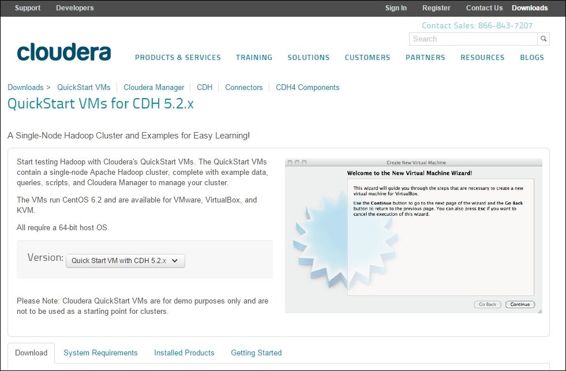
A screenshot of the Cloudera QuickStart VM download site
2. Depending on the virtual machine platform installed on your OS, choose the appropriate link (you may need to update the link as Cloudera upgrades its VMs) to download the VM file:
o To download VMWare: You can visit https://downloads.cloudera.com/demo_vm/vmware/cloudera-quickstart-vm-5.2.0-0-vmware.7z
o To download KVM: You can visit https://downloads.cloudera.com/demo_vm/kvm/cloudera-quickstart-vm-5.2.0-0-kvm.7z
o To download VirtualBox: You can visit https://downloads.cloudera.com/demo_vm/virtualbox/cloudera-quickstart-vm-5.2.0-0-virtualbox.7z
3. Next, you can start the QuickStart VM using the virtual machine platform installed on your OS. You should see the desktop of Centos 6.2 in a few minutes.

The screenshot of Cloudera QuickStart VM.
4. You can then open a terminal and type hadoop, which will display a list of functions that can operate a Hadoop cluster.
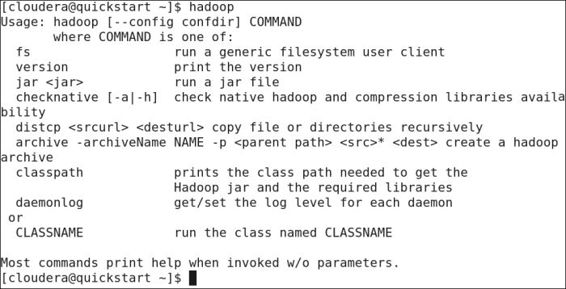
The terminal screenshot after typing hadoop
5. Open a terminal and type R. Access an R session and check whether version 3.1.1 is already installed in the Cloudera QuickStart VM. If you cannot find R installed in the VM, please use the following command to install R:
6. $ yum install R R-core R-core-devel R-devel
How it works...
Instead of building a Hadoop system on your own, you can use the Hadoop VM application provided by Cloudera (the VM is free). The QuickStart VM runs on CentOS 6.2 with a single node Apache Hadoop cluster, Hadoop Ecosystem module, and R installed. This helps you to save time, instead of requiring you to learn how to install and use Hadoop.
The QuickStart VM requires you to have a computer with a 64-bit guest OS, at least 4 GB of RAM, 3 GB of disk space, and either VMWare, VirtualBox, or KVM installed. As a result, you may not be able to use this version of VM on some computers. As an alternative, you could consider using Amazon's Elastic MapReduce instead. We will illustrate how to prepare a RHadoop environment in EMR in the last recipe of this chapter.
Setting up the Cloudera QuickStart VM is simple. Download the VM from the download site and then open the built image with either VMWare, VirtualBox, or KVM. Once you can see the desktop of CentOS, you can then access the terminal and type hadoop to see whether Hadoop is working; then, type R to see whether R works in the QuickStart VM.
See also
· Besides using the Cloudera QuickStart VM, you may consider using a Sandbox VM provided by Hontonworks or MapR. You can find Hontonworks Sandbox at http://hortonworks.com/products/hortonworks-sandbox/#installand mapR Sandbox at https://www.mapr.com/products/mapr-sandbox-hadoop/download.
Installing rmr2
The rmr2 package allows you to perform big data processing and analysis via MapReduce on a Hadoop cluster. To perform MapReduce on a Hadoop cluster, you have to install R and rmr2 on every task node. In this recipe, we will illustrate how to install rmr2 on a single node of a Hadoop cluster.
Getting ready
Ensure that you have completed the previous recipe by starting the Cloudera QuickStart VM and connecting the VM to the Internet, so that you can proceed with downloading and installing the rmr2 package.
How to do it...
Perform the following steps to install rmr2 on the QuickStart VM:
1. First, open the terminal within the Cloudera QuickStart VM.
2. Use the permission of the root to enter an R session:
3. $ sudo R
3. You can then install dependent packages before installing rmr2:
4. > install.packages(c("codetools", "Rcpp", "RJSONIO", "bitops", "digest", "functional", "stringr", "plyr", "reshape2", "rJava", "caTools"))
4. Quit the R session:
5. > q()
5. Next, you can download rmr-3.3.0 to the QuickStart VM. You may need to update the link if Revolution Analytics upgrades the version of rmr2:
6. $ wget --no-check-certificate https://raw.githubusercontent.com/RevolutionAnalytics/rmr2/3.3.0/build/rmr2_3.3.0.tar.gz
6. You can then install rmr-3.3.0 to the QuickStart VM:
7. $ sudo R CMD INSTALL rmr2_3.3.0.tar.gz
7. Lastly, you can enter an R session and use the library function to test whether the library has been successfully installed:
8. $ R
9. > library(rmr2)
How it works...
In order to perform MapReduce on a Hadoop cluster, you have to install R and RHadoop on every task node. Here, we illustrate how to install rmr2 on a single node of a Hadoop cluster. First, open the terminal of the Cloudera QuickStart VM. Before installing rmr2, we first access an R session with root privileges and install dependent R packages.
Next, after all the dependent packages are installed, quit the R session and use the wget command in the Linux shell to download rmr-3.3.0 from GitHub to the local filesystem. You can then begin the installation of rmr2. Lastly, you can access an R session and use the library function to validate whether the package has been installed.
See also
· To see more information and read updates about RHadoop, you can refer to the RHadoop wiki page hosted on GitHub: https://github.com/RevolutionAnalytics/RHadoop/wiki
Installing rhdfs
The rhdfs package is the interface between R and HDFS, which allows users to access HDFS from an R console. Similar to rmr2, one should install rhdfs on every task node, so that one can access HDFS resources through R. In this recipe, we will introduce how to install rhdfs on the Cloudera QuickStart VM.
Getting ready
Ensure that you have completed the previous recipe by starting the Cloudera QuickStart VM and connecting the VM to the Internet, so that you can proceed with downloading and installing the rhdfs package.
How to do it...
Perform the following steps to install rhdfs:
1. First, you can download rhdfs 1.0.8 from GitHub. You may need to update the link if Revolution Analytics upgrades the version of rhdfs:
2. $wget --no-check-certificate https://raw.github.com/RevolutionAnalytics/rhdfs/master/build/rhdfs_1.0.8.tar.gz
2. Next, you can install rhdfs under the command-line mode:
3. $ sudo HADOOP_CMD=/usr/bin/hadoop R CMD INSTALL rhdfs_1.0.8.tar.gz
3. You can then set up JAVA_HOME. The configuration of JAVA_HOME depends on the installed Java version within the VM:
4. $ sudo JAVA_HOME=/usr/java/jdk1.7.0_67-cloudera R CMD javareconf
4. Last, you can set up the system environment and initialize rhdfs. You may need to update the environment setup if you use a different version of QuickStart VM:
5. $ R
6. > Sys.setenv(HADOOP_CMD="/usr/bin/hadoop")
7. > Sys.setenv(HADOOP_STREAMING="/usr/lib/hadoop-mapreduce/hadoop-
8. streaming-2.5.0-cdh5.2.0.jar")
9. > library(rhdfs)
10.> hdfs.init()
How it works...
The package, rhdfs, provides functions so that users can manage HDFS using R. Similar to rmr2, you should install rhdfs on every task node, so that one can access HDFS through the R console.
To install rhdfs, you should first download rhdfs from GitHub. You can then install rhdfs in R by specifying where the HADOOP_CMD is located. You must configure R with Java support through the command, javareconf.
Next, you can access R and configure where HADOOP_CMD and HADOOP_STREAMING are located. Lastly, you can initialize rhdfs via the rhdfs.init function, which allows you to begin operating HDFS through rhdfs.
See also
· To find where HADOOP_CMD is located, you can use the which hadoop command in the Linux shell. In most Hadoop systems, HADOOP_CMD is located at /usr/bin/hadoop.
· As for the location of HADOOP_STREAMING, the streaming JAR file is often located in /usr/lib/hadoop-mapreduce/. However, if you cannot find the directory, /usr/lib/Hadoop-mapreduce, in your Linux system, you can search the streaming JAR by using the locate command. For example:
· $ sudo updatedb
· $ locate streaming | grep jar | more
Operating HDFS with rhdfs
The rhdfs package is an interface between Hadoop and R, which can call an HDFS API in the backend to operate HDFS. As a result, you can easily operate HDFS from the R console through the use of the rhdfs package. In the following recipe, we will demonstrate how to use the rhdfs function to manipulate HDFS.
Getting ready
To proceed with this recipe, you need to have completed the previous recipe by installing rhdfs into R, and validate that you can initial HDFS via the hdfs.init function.
How to do it...
Perform the following steps to operate files stored on HDFS:
1. Initialize the rhdfs package:
2. > Sys.setenv(HADOOP_CMD="/usr/bin/hadoop")
3. > Sys.setenv(HADOOP_STREAMING="/usr/lib/hadoop-mapreduce/hadoop-streaming-2.5.0-cdh5.2.0.jar")
4. > library(rhdfs)
5. > hdfs.init ()
2. You can then manipulate files stored on HDFS, as follows:
o hdfs.put: Copy a file from the local filesystem to HDFS:
o > hdfs.put('word.txt', './')
o hdfs.ls: Read the list of directory from HDFS:
o > hdfs.ls('./')
o hdfs.copy: Copy a file from one HDFS directory to another:
o > hdfs.copy('word.txt', 'wordcnt.txt')
o hdfs.move : Move a file from one HDFS directory to another:
o > hdfs.move('wordcnt.txt', './data/wordcnt.txt')
o hdfs.delete: Delete an HDFS directory from R:
o > hdfs.delete('./data/')
o hdfs.rm: Delete an HDFS directory from R:
o > hdfs.rm('./data/')
o hdfs.get: Download a file from HDFS to a local filesystem:
o > hdfs.get(word.txt', '/home/cloudera/word.txt')
o hdfs.rename: Rename a file stored on HDFS:
o hdfs.rename('./test/q1.txt','./test/test.txt')
o hdfs.chmod: Change the permissions of a file or directory:
o > hdfs.chmod('test', permissions= '777')
o hdfs.file.info: Read the meta information of the HDFS file:
o > hdfs.file.info('./')
3. Also, you can write stream to the HDFS file:
4. > f = hdfs.file("iris.txt","w")
5. > data(iris)
6. > hdfs.write(iris,f)
7. > hdfs.close(f)
4. Lastly, you can read stream from the HDFS file:
5. > f = hdfs.file("iris.txt", "r")
6. > dfserialized = hdfs.read(f)
7. > df = unserialize(dfserialized)
8. > df
9. > hdfs.close(f)
How it works...
In this recipe, we demonstrate how to manipulate HDFS using the rhdfs package. Normally, you can use the Hadoop shell to manipulate HDFS, but if you would like to access HDFS from R, you can use the rhdfs package.
Before you start using rhdfs, you have to initialize rhdfs with hdfs.init(). After initialization, you can operate HDFS through the functions provided in the rhdfs package.
Besides manipulating HDFS files, you can exchange streams to HDFS through hdfs.read and hdfs.write. We, therefore, demonstrate how to write a data frame in R to an HDFS file, iris.txt, using hdfs.write. Lastly, you can recover the written file back to the data frame using the hdfs.read function and the unserialize function.
See also
· To initialize rhdfs, you have to set HADOOP_CMD and HADOOP_STREAMING in the system environment. Instead of setting the configuration each time you're using rhdfs, you can put the configurations in the .rprofile file. Therefore, every time you start an R session, the configuration will be automatically loaded.
Implementing a word count problem with RHadoop
To demonstrate how MapReduce works, we illustrate the example of a word count, which counts the number of occurrences of each word in a given input set. In this recipe, we will demonstrate how to use rmr2 to implement a word count problem.
Getting ready
In this recipe, we will need an input file as our word count program input. You can download the example input from https://github.com/ywchiu/ml_R_cookbook/tree/master/CH12.
How to do it...
Perform the following steps to implement the word count program:
1. First, you need to configure the system environment, and then load rmr2 and rhdfs into an R session. You may need to update the use of the JAR file if you use a different version of QuickStart VM:
2. > Sys.setenv(HADOOP_CMD="/usr/bin/hadoop")
3. > Sys.setenv(HADOOP_STREAMING="/usr/lib/hadoop-mapreduce/hadoop-streaming-2.5.0-cdh5.2.0.jar ")
4. > library(rmr2)
5. > library(rhdfs)
6. > hdfs.init()
2. You can then create a directory on HDFS and put the input file into the newly created directory:
3. > hdfs.mkdir("/user/cloudera/wordcount/data")
4. > hdfs.put("wc_input.txt", "/user/cloudera/wordcount/data")
3. Next, you can create a map function:
4. > map = function(.,lines) { keyval(
5. + unlist(
6. + strsplit(
7. + x = lines,
8. + split = " +")),
9. + 1)}
4. Create a reduce function:
5. > reduce = function(word, counts) {
6. + keyval(word, sum(counts))
7. + }
5. Call the MapReduce program to count the words within a document:
6. > hdfs.root = 'wordcount' > hdfs.data = file.path(hdfs.root, 'data')
7. > hdfs.out = file.path(hdfs.root, 'out')
8. > wordcount = function (input, output=NULL) {
9. + mapreduce(input=input, output=output, input.format="text", map=map,
10.+ reduce=reduce)
11.+ }
12.> out = wordcount(hdfs.data, hdfs.out)
6. Lastly, you can retrieve the top 10 occurring words within the document:
7. > results = from.dfs(out)
8. > results$key[order(results$val, decreasing = TRUE)][1:10]
How it works...
In this recipe, we demonstrate how to implement a word count using the rmr2 package. First, we need to configure the system environment and load rhdfs and rmr2 into R. Then, we specify the input of our word count program from the local filesystem into the HDFS directory, /user/cloudera/wordcount/data, via the hdfs.put function.
Next, we begin implementing the MapReduce program. Normally, we can divide the MapReduce program into the map and reduce functions. In the map function, we first use the strsplit function to split each line into words. Then, as the strsplit function returns a list of words, we can use the unlist function to character vectors. Lastly, we can return key-value pairs with each word as a key and the value as one. As the reduce function receives the key-value pair generated from the map function, the reduce function sums the count and returns the number of occurrences of each word (or key).
After we have implemented the map and reduce functions, we can submit our job via the mapreduce function. Normally, the mapreduce function requires four inputs, which are the HDFS input path, the HDFS output path, the map function, and the reduce function. In this case, we specify the input as wordcount/data, output as wordcount/out, map function as map, reduce function as reduce, and wrap the mapreduce call in function, wordcount. Lastly, we call the function, wordcount and store the output path in the variable, out.
We can use the from.dfs function to load the HDFS data into the results variable, which contains the mapping of words and number of occurrences. We can then generate the top 10 occurring words from the results variable.
See also
· In this recipe, we demonstrate how to write an R MapReduce program to solve a word count problem. However, if you are interested in how to write a native Java MapReduce program, you can refer to http://hadoop.apache.org/docs/current/hadoop-mapreduce-client/hadoop-mapreduce-client-core/MapReduceTutorial.html.
Comparing the performance between an R MapReduce program and a standard R program
Those not familiar with how Hadoop works may often see Hadoop as a remedy for big data processing. Some might believe that Hadoop can return the processed results for any size of data within a few milliseconds. In this recipe, we will compare the performance between an R MapReduce program and a standard R program to demonstrate that Hadoop does not perform as quickly as some may believe.
Getting ready
In this recipe, you should have completed the previous recipe by installing rmr2 into the R environment.
How to do it...
Perform the following steps to compare the performance of a standard R program and an R MapReduce program:
1. First, you can implement a standard R program to have all numbers squared:
2. > a.time = proc.time()
3. > small.ints2=1:100000
4. > result.normal = sapply(small.ints2, function(x) x^2)
5. > proc.time() - a.time
2. To compare the performance, you can implement an R MapReduce program to have all numbers squared:
3. > b.time = proc.time()
4. > small.ints= to.dfs(1:100000)
5. > result = mapreduce(input = small.ints, map = function(k,v) cbind(v,v^2))
6. > proc.time() - b.time
How it works...
In this recipe, we implement two programs to square all the numbers. In the first program, we use a standard R function, sapply, to square the sequence from 1 to 100,000. To record the program execution time, we first record the processing time before the execution in a.time, and then subtract a.time from the current processing time after the execution. Normally, the execution takes no more than 10 seconds. In the second program, we use the rmr2 package to implement a program in the R MapReduce version. In this program, we also record the execution time. Normally, this program takes a few minutes to complete a task.
The performance comparison shows that a standard R program outperforms the MapReduce program when processing small amounts of data. This is because a Hadoop system often requires time to spawn daemons, job coordination between daemons, and fetching data from data nodes. Therefore, a MapReduce program often takes a few minutes to a couple of hours to finish the execution. As a result, if you can fit your data in the memory, you should write a standard R program to solve the problem. Otherwise, if the data is too large to fit in the memory, you can implement a MapReduce solution.
See also
· In order to check whether a job will run smoothly and efficiently in Hadoop, you can run a MapReduce benchmark, MRBench, to evaluate the performance of the job:
· $ hadoop jar /usr/lib/hadoop-0.20-mapreduce/hadoop-test.jar mrbench -numRuns 50
Testing and debugging the rmr2 program
Since running a MapReduce program will require a considerable amount of time, varying from a few minutes to several hours, testing and debugging become very important. In this recipe, we will illustrate some techniques you can use to troubleshoot an R MapReduce program.
Getting ready
In this recipe, you should have completed the previous recipe by installing rmr2 into an R environment.
How to do it...
Perform the following steps to test and debug an R MapReduce program:
1. First, you can configure the backend as local in rmr.options:
2. > rmr.options(backend = 'local')
2. Again, you can execute the number squared MapReduce program mentioned in the previous recipe:
3. > b.time = proc.time()
4. > small.ints= to.dfs(1:100000)
5. > result = mapreduce(input = small.ints, map = function(k,v) cbind(v,v^2))
6. > proc.time() - b.time
3. In addition to this, if you want to print the structure information of any variable in the MapReduce program, you can use the rmr.str function:
4. > out = mapreduce(to.dfs(1), map = function(k, v) rmr.str(v))
5. Dotted pair list of 14
6. $ : language mapreduce(to.dfs(1), map = function(k, v) rmr.str(v))
7. $ : language mr(map = map, reduce = reduce, combine = combine, vectorized.reduce, in.folder = if (is.list(input)) { lapply(input, to.dfs.path) ...
8. $ : language c.keyval(do.call(c, lapply(in.folder, function(fname) { kv = get.data(fname) ...
9. $ : language do.call(c, lapply(in.folder, function(fname) { kv = get.data(fname) ...
10. $ : language lapply(in.folder, function(fname) { kv = get.data(fname) ...
11. $ : language FUN("/tmp/Rtmp813BFJ/file25af6e85cfde"[[1L]], ...)
12. $ : language unname(tapply(1:lkv, ceiling((1:lkv)/(lkv/(object.size(kv)/10^6))), function(r) { kvr = slice.keyval(kv, r) ...
13. $ : language tapply(1:lkv, ceiling((1:lkv)/(lkv/(object.size(kv)/10^6))), function(r) { kvr = slice.keyval(kv, r) ...
14. $ : language lapply(X = split(X, group), FUN = FUN, ...)
15. $ : language FUN(X[[1L]], ...)
16. $ : language as.keyval(map(keys(kvr), values(kvr)))
17. $ : language is.keyval(x)
18. $ : language map(keys(kvr), values(kvr))
19. $ :length 2 rmr.str(v)
20. ..- attr(*, "srcref")=Class 'srcref' atomic [1:8] 1 34 1 58 34 58 1 1
21. .. .. ..- attr(*, "srcfile")=Classes 'srcfilecopy', 'srcfile' <environment: 0x3f984f0>
22.v
23. num 1
How it works...
In this recipe, we introduced some debugging and testing techniques you can use while implementing the MapReduce program. First, we introduced the technique to test a MapReduce program in a local mode. If you would like to run the MapReduce program in a pseudo distributed or fully distributed mode, it would take you a few minutes to several hours to complete the task, which would involve a lot of wastage of time while troubleshooting your MapReduce program. Therefore, you can set the backend to the local mode in rmr.options so that the program will be executed in the local mode, which takes lesser time to execute.
Another debugging technique is to list the content of the variable within the map or reduce function. In an R program, you can use the str function to display the compact structure of a single variable. In rmr2, the package also provides a function named rmr.str, which allows you to print out the content of a single variable onto the console. In this example, we use rmr.str to print the content of variables within a MapReduce program.
See also
· For those who are interested in the option settings for the rmr2 package, you can refer to the help document of rmr.options:
· > help(rmr.options)
Installing plyrmr
The plyrmr package provides common operations (as found in plyr or reshape2) for users to easily perform data manipulation through the MapReduce framework. In this recipe, we will introduce how to install plyrmr on the Hadoop system.
Getting ready
Ensure that you have completed the previous recipe by starting the Cloudera QuickStart VM and connecting the VM to the Internet. Also, you need to have the rmr2 package installed beforehand.
How to do it...
Perform the following steps to install plyrmr on the Hadoop system:
1. First, you should install libxml2-devel and curl-devel in the Linux shell:
2. $ yum install libxml2-devel
3. $ sudo yum install curl-devel
2. You can then access R and install the dependent packages:
3. $ sudo R
4. > Install.packages(c(" Rcurl", "httr"), dependencies = TRUE
5. > Install.packages("devtools", dependencies = TRUE)
6. > library(devtools)
7. > install_github("pryr", "hadley")
8. > install.packages(c(" R.methodsS3", "hydroPSO"), dependencies = TRUE)
9. > q()
3. Next, you can download plyrmr 0.5.0 and install it on Hadoop VM. You may need to update the link if Revolution Analytics upgrades the version of plyrmr:
4. $ wget -no-check-certificate https://raw.github.com/RevolutionAnalytics/plyrmr/master/build/plyrmr_0.5.0.tar.gz
5. $ sudo R CMD INSTALL plyrmr_0.5.0.tar.gz
4. Lastly, validate the installation:
5. $ R
6. > library(plyrmr)
How it works...
Besides writing an R MapReduce program using the rmr2 package, you can use the plyrmr to manipulate data. The plyrmr package is similar to hive and pig in the Hadoop ecosystem, which is the abstraction of the MapReduce program. Therefore, we can implement an R MapReduce program in plyr style instead of implementing the map f and reduce functions.
To install plyrmr, first install the package of libxml2-devel and curl-devel, using the yum install command. Then, access R and install the dependent packages. Lastly, download the file from GitHub and install plyrmr in R.
See also
· To read more information about plyrmr, you can use the help function to refer to the following document:
· > help(package=plyrmr)
Manipulating data with plyrmr
While writing a MapReduce program with rmr2 is much easier than writing a native Java version, it is still hard for nondevelopers to write a MapReduce program. Therefore, you can use plyrmr, a high-level abstraction of the MapReduce program, so that you can use plyr-like operations to manipulate big data. In this recipe, we will introduce some operations you can use to manipulate data.
Getting ready
In this recipe, you should have completed the previous recipes by installing plyrmr and rmr2 in R.
How to do it...
Perform the following steps to manipulate data with plyrmr:
1. First, you need to load both plyrmr and rmr2 into R:
2. > library(rmr2)
3. > library(plyrmr)
2. You can then set the execution mode to the local mode:
3. > plyrmr.options(backend="local")
3. Next, load the Titanic dataset into R:
4. > data(Titanic)
5. > titanic = data.frame(Titanic)
4. Begin the operation by filtering the data:
5. > where(
6. + Titanic,
7. + Freq >=100)
5. You can also use a pipe operator to filter the data:
6. > titanic %|% where(Freq >=100)
6. Put the Titanic data into HDFS and load the path of the data to the variable, tidata:
7. > tidata = to.dfs(data.frame(Titanic), output = '/tmp/titanic')
8. > tidata
7. Next, you can generate a summation of the frequency from the Titanic data:
8. > input(tidata) %|% transmute(sum(Freq))
8. You can also group the frequency by sex:
9. > input(tidata) %|% group(Sex) %|% transmute(sum(Freq))
9. You can then sample 10 records out of the population:
10.> sample(input(tidata), n=10)
10.In addition to this, you can use plyrmr to join two datasets:
11.> convert_tb = data.frame(Label=c("No","Yes"), Symbol=c(0,1))
12.ctb = to.dfs(convert_tb, output = 'convert')
13.> as.data.frame(plyrmr::merge(input(tidata), input(ctb), by.x="Survived", by.y="Label"))
14.> file.remove('convert')
How it works...
In this recipe, we introduce how to use plyrmr to manipulate data. First, we need to load the plyrmr package into R. Then, similar to rmr2, you have to set the backend option of plyrmr as the local mode. Otherwise, you will have to wait anywhere between a few minutes to several hours if plyrmr is running on Hadoop mode (the default setting).
Next, we can begin the data manipulation with data filtering. You can choose to call the function nested inside the other function call in step 4. On the other hand, you can use the pipe operator, %|%, to chain multiple operations. Therefore, we can filter data similar to step 4, using pipe operators in step 5.
Next, you can input the dataset into either the HDFS or local filesystem, using to.dfs in accordance with the current running mode. The function will generate the path of the dataset and save it in the variable, tidata. By knowing the path, you can access the data using the input function. Next, we illustrate how to generate a summation of the frequency from the Titanic dataset with the transmute and sum functions. Also, plyrmr allows users to sum up the frequency by gender.
Additionally, in order to sample data from a population, you can also use the sample function to select 10 records out of the Titanic dataset. Lastly, we demonstrate how to join two datasets using the merge function from plyrmr.
See also
Here we list some functions that can be used to manipulate data with plyrmr. You may refer to the help function for further details on their usage and functionalities:
· Data manipulation:
o bind.cols: This adds new columns
o select: This is used to select columns
o where: This is used to select rows
o transmute: This uses all of the above plus their summaries
· From reshape2:
o melt and dcast: It converts long and wide data frames
· Summary:
o count
o quantile
o sample
· Extract:
o top.k
o bottom.k
Conducting machine learning with RHadoop
In the previous chapters, we have demonstrated how powerful R is when used to solve machine learning problems. Also, we have shown that the use of Hadoop allows R to process big data in parallel. At this point, some may believe that the use of RHadoop can easily solve machine learning problems of big data via numerous existing machine learning packages. However, you cannot use most of these to solve machine learning problems as they cannot be executed in the MapReduce mode. In the following recipe, we will demonstrate how to implement a MapReduce version of linear regression and compare this version with the one using the lm function.
Getting ready
In this recipe, you should have completed the previous recipe by installing rmr2 into the R environment.
How to do it...
Perform the following steps to implement a linear regression in MapReduce:
1. First, load the cats dataset from the MASS package:
2. > library(MASS)
3. > data(cats)
4. > X = matrix(cats$Bwt)
5. > y = matrix(cats$Hwt)
2. You can then generate a linear regression model by calling the lm function:
3. > model = lm(y~X)
4. > summary(model)
5.
6. Call:
7. lm(formula = y ~ X)
8.
9. Residuals:
10. Min 1Q Median 3Q Max
11.-3.5694 -0.9634 -0.0921 1.0426 5.1238
12.
13.Coefficients:
14. Estimate Std. Error t value Pr(>|t|)
15.(Intercept) -0.3567 0.6923 -0.515 0.607
16.X 4.0341 0.2503 16.119 <2e-16 ***
17.---
18.Signif. codes:
19.0 '***' 0.001 '**' 0.01 '*' 0.05 '.' 0.1 ' ' 1
20.
21.Residual standard error: 1.452 on 142 degrees of freedom
22.Multiple R-squared: 0.6466, Adjusted R-squared: 0.6441
23.F-statistic: 259.8 on 1 and 142 DF, p-value: < 2.2e-16
3. You can now make a regression plot with the given data points and model:
4. > plot(y~X)
5. > abline(model, col="red")
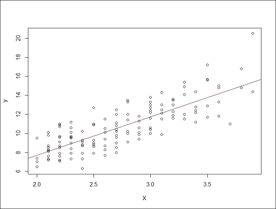
Linear regression plot of cats dataset
4. Load rmr2 into R:
5. > Sys.setenv(HADOOP_CMD="/usr/bin/hadoop")
6. > Sys.setenv(HADOOP_STREAMING="/usr/lib/hadoop-mapreduce/hadoop-> streaming-2.5.0-cdh5.2.0.jar")
7. > library(rmr2)
8. > rmr.options(backend="local")
5. You can then set up X and y values:
6. > X = matrix(cats$Bwt)
7. > X.index = to.dfs(cbind(1:nrow(X), X))
8. > y = as.matrix(cats$Hwt)
6. Make a Sum function to sum up the values:
7. > Sum =
8. + function(., YY)
9. + keyval(1, list(Reduce('+', YY)))
7. Compute Xtx in MapReduce, Job1:
8. > XtX =
9. + values(
10.+ from.dfs(
11.+ mapreduce(
12.+ input = X.index,
13.+ map =
14.+ function(., Xi) {
15.+ Xi = Xi[,-1]
16.+ keyval(1, list(t(Xi) %*% Xi))},
17.+ reduce = Sum,
18.+ combine = TRUE)))[[1]]
8. You can then compute Xty in MapReduce, Job2:
9. Xty =
10.+ values(
11.+ from.dfs(
12.+ mapreduce(
13.+ input = X.index,
14.+ map = function(., Xi) {
15.+ yi = y[Xi[,1],]
16.+ Xi = Xi[,-1]
17.+ keyval(1, list(t(Xi) %*% yi))},
18.+ reduce = Sum,
19.+ combine = TRUE)))[[1]]
9. Lastly, you can derive the coefficient from XtX and Xty:
10.> solve(XtX, Xty)
11. [,1]
12.[1,] 3.907113
How it works...
In this recipe, we demonstrate how to implement linear logistic regression in a MapReduce fashion in R. Before we start the implementation, we review how traditional linear models work. We first retrieve the cats dataset from the MASS package. We then load X as the body weight (Bwt) and y as the heart weight (Hwt).
Next, we begin to fit the data into a linear regression model using the lm function. We can then compute the fitted model and obtain the summary of the model. The summary shows that the coefficient is 4.0341 and the intercept is -0.3567. Furthermore, we draw a scatter plot in accordance with the given data points and then draw a regression line on the plot.
As we cannot perform linear regression using the lm function in the MapReduce form, we have to rewrite the regression model in a MapReduce fashion. Here, we would like to implement a MapReduce version of linear regression in three steps, which are: calculate the Xtx value with the MapReduce, job1, calculate the Xty value with MapReduce, job2, and then derive the coefficient value:
· In the first step, we pass the matrix, X, as the input to the map function. The map function then calculates the cross product of the transposed matrix, X, and, X. The reduce function then performs the sum operation defined in the previous section.
· In the second step, the procedure of calculating Xty is similar to calculating XtX. The procedure calculates the cross product of the transposed matrix, X, and, y. The reduce function then performs the sum operation.
· Lastly, we use the solve function to derive the coefficient, which is 3.907113.
As the results show, the coefficients computed by lm and MapReduce differ slightly. Generally speaking, the coefficient computed by the lm model is more accurate than the one calculated by MapReduce. However, if your data is too large to fit in the memory, you have no choice but to implement linear regression in the MapReduce version.
See also
· You can access more information on machine learning algorithms at: https://github.com/RevolutionAnalytics/rmr2/tree/master/pkg/tests
Configuring RHadoop clusters on Amazon EMR
Until now, we have only demonstrated how to run a RHadoop program in a single Hadoop node. In order to test our RHadoop program on a multi-node cluster, the only thing you need to do is to install RHadoop on all the task nodes (nodes with either task tracker for mapreduce version 1 or node manager for map reduce version 2) of Hadoop clusters. However, the deployment and installation is time consuming. On the other hand, you can choose to deploy your RHadoop program on Amazon EMR, so that you can deploy multi-node clusters and RHadoop on every task node in only a few minutes. In the following recipe, we will demonstrate how to configure RHadoop cluster on an Amazon EMR service.
Getting ready
In this recipe, you must register and create an account on AWS, and you also must know how to generate a EC2 key-pair before using Amazon EMR.
For those who seek more information on how to start using AWS, please refer to the tutorial provided by Amazon at http://docs.aws.amazon.com/AWSEC2/latest/UserGuide/EC2_GetStarted.html.
How to do it...
Perform the following steps to configure RHadoop on Amazon EMR:
1. First, you can access the console of the Amazon Web Service (refer to https://us-west-2.console.aws.amazon.com/console/) and find EMR in the analytics section. Then, click on EMR.
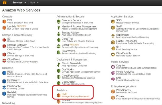
Access EMR service from AWS console.
2. You should find yourself in the cluster list of the EMR dashboard (refer to https://us-west-2.console.aws.amazon.com/elasticmapreduce/home?region=us-west-2#cluster-list::); click on Create cluster.
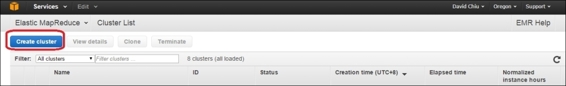
Cluster list of EMR
3. Then, you should find yourself on the Create Cluster page (refer to https://us-west-2.console.aws.amazon.com/elasticmapreduce/home?region=us-west-2#create-cluster:).
4. Next, you should specify Cluster name and Log folder S3 location in the cluster configuration.
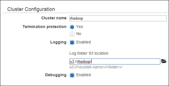
Cluster configuration in the create cluster page
5. You can then configure the Hadoop distribution on Software Configuration.

Configure the software and applications
6. Next, you can configure the number of nodes within the Hadoop cluster.
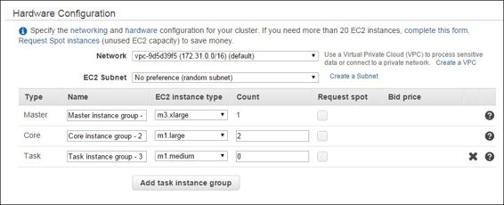
Configure the hardware within Hadoop cluster
7. You can then specify the EC2 key-pair for the master node login.
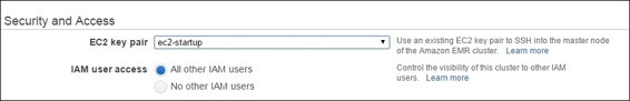
Security and access to the master node of the EMR cluster
8. To set up RHadoop, one has to perform bootstrap actions to install RHadoop on every task node. Please write a file named bootstrapRHadoop.sh, and insert the following lines within the file:
9. echo 'install.packages(c("codetools", "Rcpp", "RJSONIO", "bitops", "digest", "functional", "stringr", "plyr", "reshape2", "rJava", "caTools"), repos="http://cran.us.r-project.org")' > /home/hadoop/installPackage.R
10.sudo Rscript /home/hadoop/installPackage.R
11.wget --no-check-certificate https://raw.githubusercontent.com/RevolutionAnalytics/rmr2/master/build/rmr2_3.3.0.tar.gz
12.sudo R CMD INSTALL rmr2_3.3.0.tar.gz
13.wget --no-check-certificate https://raw.github.com/RevolutionAnalytics/rhdfs/master/build/rhdfs_1.0.8.tar.gz
sudo HADOOP_CMD=/home/hadoop/bin/hadoop R CMD INSTALL rhdfs_1.0.8.tar.gz
9. You should upload bootstrapRHadoop.sh to S3.
10.You now need to add the bootstrap action with Custom action, and add s3://<location>/bootstrapRHadoop.sh within the S3 location.
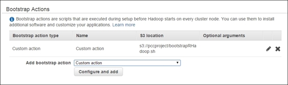
Set up the bootstrap action
11.Next, you can click on Create cluster to launch the Hadoop cluster.
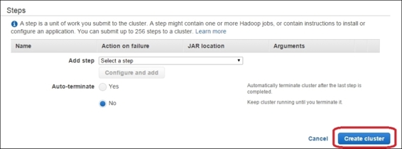
Create the cluster
12.Lastly, you should see the master public DNS when the cluster is ready. You can now access the terminal of the master node with your EC2-key pair:
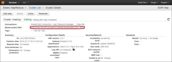
A screenshot of the created cluster
How it works...
In this recipe, we demonstrate how to set up RHadoop on Amazon EMR. The benefit of this is that you can quickly create a scalable, on demand Hadoop with just a few clicks within a few minutes. This helps save you time from building and deploying a Hadoop application. However, you have to pay for the number of running hours for each instance. Before using Amazon EMR, you should create an AWS account and know how to set up the EC2 key-pair and the S3. You can then start installing RHadoop on Amazon EMR.
In the first step, access the EMR cluster list and click on Create cluster. You can see a list of configurations on the Create cluster page. You should then set up the cluster name and log folder in the S3 location in the cluster configuration.
Next, you can set up the software configuration and choose the Hadoop distribution you would like to install. Amazon provides both its own distribution and the MapR distribution. Normally, you would skip this section unless you have concerns about the default Hadoop distribution.
You can then configure the hardware by specifying the master, core, and task node. By default, there is only one master node, and two core nodes. You can add more core and task nodes if you like. You should then set up the key-pair to login to the master node.
You should next make a file containing all the start scripts named bootstrapRHadoop.sh. After the file is created, you should save the file in the S3 storage. You can then specify custom action in Bootstrap Action with bootstrapRHadoop.sh as the Bootstrap script. Lastly, you can click on Create cluster and wait until the cluster is ready. Once the cluster is ready, one can see the master public DNS and can use the EC2 key-pair to access the terminal of the master node.
Beware! Terminate the running instance if you do not want to continue using the EMR service. Otherwise, you will be charged per instance for every hour you use.
See also
· Google also provides its own cloud solution, the Google compute engine. For those who would like to know more, please refer to https://cloud.google.com/compute/.
All materials on the site are licensed Creative Commons Attribution-Sharealike 3.0 Unported CC BY-SA 3.0 & GNU Free Documentation License (GFDL)
If you are the copyright holder of any material contained on our site and intend to remove it, please contact our site administrator for approval.
© 2016-2026 All site design rights belong to S.Y.A.