Test Scoring and Analysis Using SAS (2014)

Chapter 7. Assessing Test Reliability

Introduction

Test reliability is a measure of repeatability. A test would not be very useful if, upon repeat administrations, a person’s score varied widely. Intuitively, test reliability is related to test length. You would not expect a test of only a few items to be highly reliable because a person could make a few accurate guesses and obtain a high score or make a few bad guesses and obtain a low score.

One of the classic methods of assessing test reliability is called test-retest reliability. A group of subjects takes a test and, at some future time, typically a few weeks, retakes the same test. The time interval between the test and retest needs to be long enough so that the student does not remember her answer to each of the items but short enough so that the student has not either learned or forgotten material related to the test. You would expect the scores on the two administrations of the test to be related (correlated). The degree of correlation between the scores on the two test administrations is called test-retest reliability.

Because it is often impractical to administer a test a second time, several methods of assessing reliability have been developed that involve a single administration of the test. These methods include split-half reliability, the Kuder-Richardson Formula 20, and Chronbach’s Alpha. These methods are discussed in this chapter, along with SAS programs to compute them.

Computing Split-Half Reliability

In the early days before computers were available, a common method of assessing test reliability was called split-half reliability. The concept was straightforward: You would split the test in half (usually by choosing the odd-numbered items as one test and the even-numbered items as a second test). You would then score each of the halves and compute the correlation between the two scores. Since longer tests tend to be more reliable than shorter tests, a formula developed by Spearman and Brown, called the Spearman-Brown prophecy formula, computes the reliability of a test that is shorter or longer than the one on which the reliability is measured. The formula is:

where is the estimated correlation for a test that is N times longer (or shorter) than the given test and is the correlation of the original test.

Because a split-half correlation is assessed on a test half the length of the original, you can apply the Spearman-Brown formula to make the adjustment, like this:

where is the estimated correlation and is the split-half correlation. Although this method is no longer used (now that we have computers), it is still interesting to compute this statistic. If nothing else, it makes for some interesting SAS programming.

The first step in computing a split-half correlation is to divide the test in half and score the two halves. Here is the program:

Program 7.1: Computing the Score for the Odd- and Even-Numbered Items

*Split-Half Reliability;

data split_half;

set score;

array ans[56] $ 1;

array key[56] $ 1;

array score[56];

*Score odd items;

Raw_Odd = 0;

Raw_Even = 0;

do Item = 1 to 55 by 2;

Score[Item] = ans[Item] eq key[Item];

Raw_odd + Score[Item];

end;

*Score even items;

do Item = 2 to 56 by 2;

Score[Item] = ans[Item] eq key[Item];

Raw_Even + Score[Item];

end;

keep ID Raw:;

run;

A quick programming note: The expression Raw in the KEEP statement is a short-cut way of referring to all variables that begin with the characters Raw.

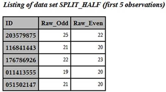
Here is a listing of the first five observations in data set SPLIT_HALF:

First Five Observations from Data Set SPLIT_HALF

You can now compute a correlation between the odd and even scores, using PROC CORR:

Program 7.2: Computing the Correlation Between the Odd and Even Scores

title "Computing the Correlation Between the Odd and Even Tests";

proc corr data=split_half nosimple;

var Raw_Odd Raw_Even;

run;

Here is the result:

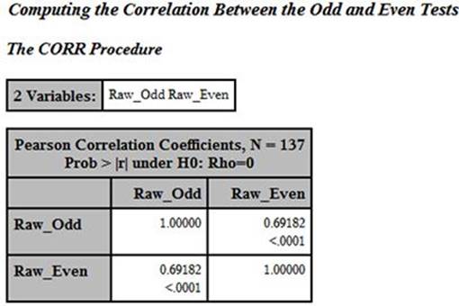
The correlation between the Odd and Even items is .69182. The only task left is to adjust this correlation using the Spearman-Brown formula. This can be done by hand or in a short SAS DATA step. We will, of course, choose the programming solution, which looks like this:

Program 7.3: Computing the Spearman-Brown Adjusted Split-Half Correlation

*Using PROC CORR to output the split half value to

a data set so that the Spearman-Brown prophcy formula

can be applied;

proc corr data=split_half nosimple noprint

outp=corrout(where=(_type_='CORR' and _NAME_='Raw_Odd'));

var Raw_Odd Raw_Even;

run;

data _null_;

file print;

set corrout(keep=Raw_Even);

Odd_Even_Adjusted= 2*Raw_Even / (1 + Raw_Even);

put (Raw_Even Odd_Even_Adjusted)(= 7.3);

run;

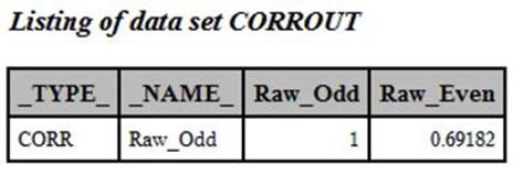
You use the procedure option, OUTP=, to have PROC CORR output values to a SAS data set. This data set contains variables _TYPE_ and _NAME_, added by the procedure. If you wish to see the contents of this data set, you can run the PROC CORR portion of Program 7.3, without the data set options (that are used to subset the output data set to just those values you want). The correlation coefficient you want in the output data set has a value of _TYPE_ equal to ‘CORR’ and a value of _NAME_ equal to ‘Raw_Odd’. To help understand this program, here is a listing of data set CORROUT, produced by PROC CORR:

Listing of Data Set CORROUT

All that is left to do is to apply the Spearman-Brown formula in a DATA step and output the values of Raw_Even and the adjusted value of this coefficient.

An aside: Because you want to print out values in this DATA step but do not need the data set once you have printed the values, you use the special data set name _NULL_. This is a data set that is not a data set—that is, a SAS data set is not being created. Whenever you want to compute some values in a DATA step and plan to use PUT statements to output these values to files or to the output device, it is not necessary to create an actual data set, so using DATA _NULL_ is very efficient. By not creating a real data set, you reduce all the overhead required to write the data to a physical disk.

Here is the result of the PUT statement in the DATA _NULL_ step above:

Raw_Even=0.692 Odd_Even_Adjusted=0.818

The adjusted value for the split-half correlation is .818. That value is considered quite good for a typical in-class assessment test.

Computing Kuder-Richardson Formula 20 (KR-20)

Researchers G.F. Kuder and M.W. Richardson developed a formula to measure internal consistency reliability for measures with dichotomous choices. Known as the Kuder-Richardson Formula 20, it is similar to a split-half correlation, but it can be thought of as the mean split-half correlation if the test is divided in two in all possible ways. (This is not exactly true but makes for a good mental image of what is going on.) The KR-20 formula is:

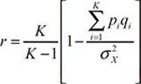
where K is the number of items on the test, p_i is the item difficulty (the proportion of the class that answered the item correctly), q_i is 1 – p_i, and is the variance of the test scores.

You can use PROC MEANS to compute the two variances used in the formula and output them to a SAS data set, as follows:

Program 7.4: Computing the Variances to Compute KR-20

proc means data=score noprint;

output out=variance var=Raw_Var Item_Var1-Item_Var56;

var Raw Score1-Score56;

run;

You use the keyword VAR= to output variances. Raw_Var is the variance of the test score (Raw), and the variables Item_Var1 to Item_Var56 are the item variances, which will be summed. You can now write a short DATA step to compute KR-20.

Program 7.5: Computing the Kuder-Richardson Formula 20

title “Computing the Kuder-Richardson Formula 20”;

data _null_;

file print;

set variance;

array Item_Var[56];

do i = 1 to 56;

Item_Variance + Item_Var[i];

end;

KR_20 = (56/55)*(1 - Item_Variance/Raw_Var);

put (KR_20 Item_Variance Raw_Var)(= 7.3);

drop i;

run;

You use a DO loop to sum the item variances. The expression Item_Variance + Item+Var[i] is a SUM statement because it is of the form VARIABLE + EXPRESSION. This has some differences from an ASSIGNMENT statement where you use an equal sign to assign a value to a variable. It is important to remember that a SUM statement has the following properties. First, the VARIABLE is automatically retained. Second, the VARIABLE is initialized to 0. Third, if the EXPRESSION is a missing value, it is ignored. The result of the DO loop is that the variable Item_Variance is the sum of the item variances. All that is left to do is to compute KR-20 and write it out to the Output window. The output looks like this:

Computing the Kuder-Richard Formula 20

KR_20=0.798 Item_Variance=7.902 Raw_Var=36.551

Computing Cronbach’s Alpha

The KR-20 formula is applicable to tests where the item scores are dichotomous (right or wrong). A generalization of this formula, called Cronbach’s Alpha, can be used for scaled items such as items on a Likert scale. Fortunately, you can use the ALPHA option with PROC CORR to compute this value. Cronbach’s Alpha is equivalent to the KR-20 for dichotomous items. Here is the SAS code to compute Cronbach’s Alpha, followed by the output:

Program 7.6: Computing Cronbach's Alpha

*Cronbach's Alpha;

proc corr data=score nosimple noprint alpha

outp=Chronbach(where=(_type_='RAWALPHA') keep=_type_ Score1

rename=(Score1=Alpha));

var Score1-Score56;

run;

Output from Program 7.6

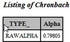
Notice that the value of Chronbach's Alpha is identical to the KR-20 value computed earlier. Even if you have a test with dichotomous items, you may elect to use PROC CORR with the ALPHA option instead of the SAS code demonstrated in Programs 7.4 and 7.5.

Demonstrating the Effect of Item Discrimination on Test Reliability

There is a relationship between item discrimination and test reliability—the higher your item discrimination indices, the higher your overall test reliability will be. One way to demonstrate this is to rescore the statistics test we have been using, after removing four items with very low point-biserial coefficients. The following table shows the item statistics for these four items:

Four Items on the Statistics Test with Poor Item Statistics

Notice that the point-biserial correlation coefficients are either very close to 0 or negative. The original reliability for this test was as follows:

KR_20=0.798 Item_Variance=7.902 Raw_Var=36.551

You can use the macro programs in Chapter 11 to score the original test, rescore that test with the four items that performed poorly removed, and then compute the reliability of the rescored test. To start, you can use the SCORE_TEXT program to score the original statistics test as follows:

%score_text(%score_text(file='c:\books\test scoring\stat_test.txt',

dsn=score_stat,

length_id=9,

Start=11,

Nitems=56)

Next, use the %RESCORE macro to rescore this test as follows:

%Rescore(Dsn=Score_stat,

Dsn_Rescore=New_Stat,

Nitems=56,

List=8 26 43 54)

Now that you have rescored the test, you can run the KR_20 macro to compute the Kuder-Richardson reliability, like this:

%KR_20(Dsn=New_Stat,

Nitems=52)

Here are the results:

KR_20=0.818 Item_Variance=7.225 Raw_Var=36.503

The reliability, as measured by the KR-20, is higher, even though the test is now four items shorter.

Demonstrating the Effect of Test Length on Test Reliability

As discussed earlier, longer tests tend to be more reliable. To demonstrate this, the odd and even items of the 56-item statistics test were scored separately and the KR-20 was computed for each subtest, with the following results:

Computing the Kuder-Richardson Formula 20

Reliability of Test Selecting Odd Numbered Items

KR_20=0.685 Item_Variance=4.099 Raw_Var=12.063

Computing the Kuder-Richardson Formula 20

Reliability of Test Selecting Even Numbered Items

KR_20=0.626 Item_Variance=3.803 Raw_Var=9.599

The KR-20 for the entire test was .798. If we take the mean KR-20 from the odd and even test versions and apply the Spearman-Brown prophecy formula to estimate the reliability of a test twice as long, the result is .7915, quite close to the actual value.

Conclusion

Once you have completed your item analysis, it's time to estimate the overall test reliability. For dichotomous items (right or wrong), Kuder-Richardson's formula 20 and Cronbach's Alpha are equivalent and give you a good indication of your test's reliability. If you determine that either of these coefficients is too low, the next step is to attempt to rewrite items that have low point-biserial coefficients and, possibly, to increase the length of the test by writing new items.