Time Series Databases: New Ways to Store and Access Data (2014)

Chapter 1. Time Series Data: Why Collect It?

“Collect your data as if your life depends on it!”

This bold admonition may seem like a quote from an overzealous project manager who holds extreme views on work ethic, but in fact, sometimes your life does depend on how you collect your data. Time series data provides many such serious examples. But let’s begin with something less life threatening, such as: where would you like to spend your vacation?

Suppose you’ve been living in Seattle, Washington for two years. You’ve enjoyed a lovely summer, but as the season moves into October, you are not looking forward to what you expect will once again be a gray, chilly, and wet winter. As a break, you decide to treat yourself to a short holiday in December to go someplace warm and sunny. Now begins the search for a good destination.

You want sunshine on your holiday, so you start by seeking out reports for rainfall in potential vacation places. Reasoning that an average of many measurements will provide a more accurate report than just checking what is happening at the moment, you compare the yearly rainfall average for the Caribbean country of Costa Rica (about 77 inches or 196 cm) with that of the South American coastal city of Rio de Janeiro, Brazil (46 inches or 117cm). Seeing that Costa Rica gets almost twice as much rain per year on average than Rio de Janeiro, you choose the Brazilian city for your December trip and end up slightly disappointed when it rains all four days of your holiday.

The probability of choosing a sunny destination for December might have been better if you had looked at rainfall measurements recorded with the time at which they were made throughout the year rather than just an annual average. A pattern of rainfall would be revealed, as shown inFigure 1-1. With this time series style of data collection, you could have easily seen that in December you were far more likely to have a sunny holiday in Costa Rica than in Rio, though that would certainly not have been true for a September trip.

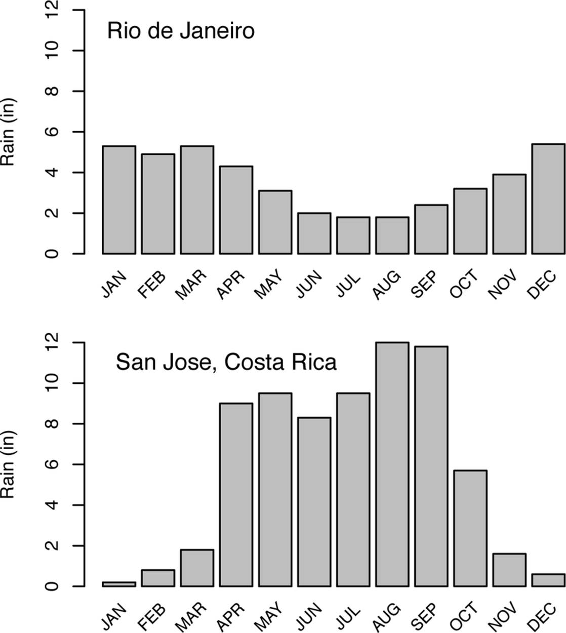
Figure 1-1. These graphs show the monthly rainfall measurements for Rio de Janeiro, Brazil, and San Jose, Costa Rica. Notice the sharp reduction in rainfall in Costa Rica going from September–October to December–January. Despite a higher average yearly rainfall in Costa Rica, its winter months of December and January are generally drier than those months in Rio de Janeiro (or for that matter, in Seattle).

This small-scale, lighthearted analogy hints at the useful insights possible when certain types of data are recorded as a time series—as measurements or observations of events as a function of the time at which they occurred. The variety of situations in which time series are useful is wide ranging and growing, especially as new technologies are producing more data of this type and as new tools are making it feasible to make use of time series data at large scale and in novel applications. As we alluded to at the start, recording the exact time at which a critical parameter was measured or a particular event occurred can have a big impact on some very serious situations such as safety and risk reduction. The airline industry is one such example.

Recording the time at which a measurement was made can greatly expand the value of the data being collected. We have all heard of the flight data recorders used in airplane travel as a way to reconstruct events after a malfunction or crash. Oddly enough, the public sometimes calls them “black boxes,” although they are generally painted a bright color such as orange. A modern aircraft is equipped with sensors to measure and report data many times per second for dozens of parameters throughout the flight. These measurements include altitude, flight path, engine temperature and power, indicated air speed, fuel consumption, and control settings. Each measurement includes the time it was made. In the event of a crash or serious accident, the events and actions leading up to the crash can be reconstructed in exquisite detail from these data.

Flight sensor data is not only used to reconstruct events that precede a malfunction. Some of this sensor data is transferred to other systems for analysis of specific aspects of flight performance in order for the airline company to optimize operations and maintain safety standards and for the equipment manufacturers to track the behavior of specific components along with their microenvironment, such as vibration, temperature, or pressure. Analysis of these time series datasets can provide valuable insights that include how to improve fuel consumption, change recommended procedures to reduce risk, and how best to schedule maintenance and equipment replacement. Because the time of each measurement is recorded accurately, it’s possible to correlate many different conditions and events. Figure 1-2 displays time series data, the altitude data from flight data systems of a number of aircraft taking off from San Jose, California.

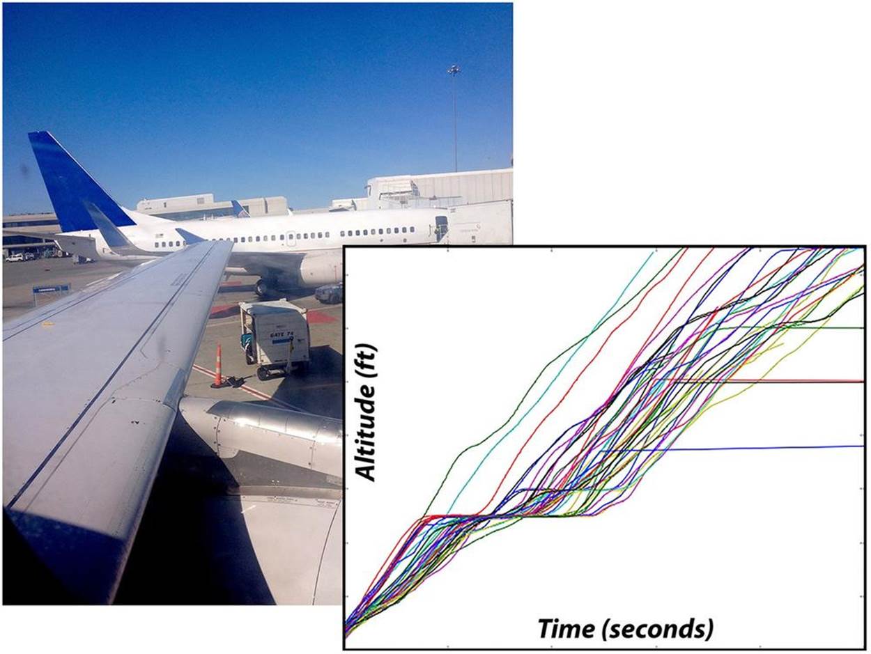
Figure 1-2. Dynamic systems such as aircraft produce a wide variety of data that can and should be stored as a time series to reap the maximum benefit from analytics, especially if the predominant access pattern for queries is based on a time range. The chart shows the first few minutes of altitude data from the flight data systems of aircraft taking off at a busy airport in California.

To clarify the concept of a time series, let’s first consider a case where a time series is not necessary. Sometimes you just want to know the value of a particular parameter at the current moment. As a simple example, think about glancing at the speedometer in a car while driving. What’s of interest in this situation is to know the speed at the moment, rather than having a history of how that condition has changed with time. In this case, a time series of speed measurements is not of interest to the driver.

Next, consider how you think about time. Going back to the analogy of a holiday flight for a moment, sometimes you are concerned with the length of a time interval --how long is the flight in hours, for instance. Once your flight arrives, your perception likely shifts to think of time as anabsolute reference: your connecting flight leaves at 10:42 am, your meeting begins at 1:00 pm, etc. As you travel, time may also represent a sequence. Those people who arrive earlier than you in the taxi line are in front of you and catch a cab while you are still waiting.

Time as interval, as an ordering principle for a sequence, as absolute reference—all of these ways of thinking about time can also be useful in different contexts. Data collected as a time series is likely more useful than a single measurement when you are concerned with the absolute time at which a thing occurred or with the order in which particular events happened or with determining rates of change. But note that time series data tells you when something happened, not necessarily when you learned about it, because data may be recorded long after it is measured. (To tell when you knew certain information, you would need a bi-temporal database, which is beyond the scope of this book.) With time series data, not only can you determine the sequence in which events happened, you also can correlate different types of events or conditions that co-occur. You might want to know the temperature and vibrations in a piece of equipment on an airplane as well as the setting of specific controls at the time the measurements were made. By correlating different time series, you may be able to determine how these conditions correspond.

The basis of a time series is the repeated measurement of parameters over time together with the times at which the measurements were made. Time series often consist of measurements made at regular intervals, but the regularity of time intervals between measurements is not a requirement. Also, the data collected is very commonly a number, but again, that is not essential. Time series datasets are typically used in situations in which measurements, once made, are not revised or updated, but rather, where the mass of measurements accumulates, with new data added for each parameter being measured at each new time point. These characteristics of time series limit the demands we put on the technology we use to store time series and thus affect how we design that technology. Although some approaches for how best to store, access, and analyze this type of data are relatively new, the idea of time series data is actually quite an old one.

Time Series Data Is an Old Idea

It may surprise you to know that one of the great examples of the advantages to be reaped from collecting data as a time series—and doing it as a crowdsourced, open source, big data project—comes from the mid-19th century. The story starts with a sailor named Matthew Fontaine Maury, who came to be known as the Pathfinder of the Seas. When a leg injury forced him to quit ocean voyages in his thirties, he turned to scientific research in meteorology, astronomy, oceanography, and cartography, and a very extensive bit of whale watching, too.

Ship’s captains and science officers had long been in the habit of keeping detailed logbooks during their voyages. Careful entries included the date and often the time of various measurements, such as how many knots the ship was traveling, calculations of latitude and longitude on specific days, and observations of ocean conditions, wildlife, weather, and more. A sample entry in a ship’s log is shown in Figure 1-3.

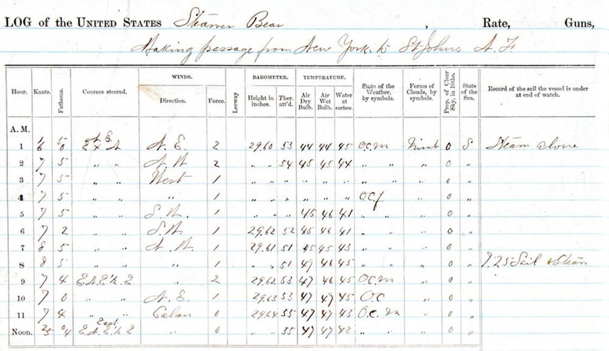
Figure 1-3. Old ship’s log of the Steamship Bear as it steamed north as part of the 1884 Greely rescue mission to the arctic. Nautical logbooks are an early source of large-scale time series data.^[1^]

Maury saw the hidden value in these logs when analyzed collectively and wanted to bring that value to ships’ captains. When Maury was put in charge of the US Navy’s office known as the Depot of Charts and Instruments, he began a project to extract observations of winds and currents accumulated over many years in logbooks from many ships. He used this time series data to carry out an analysis that would enable him to recommend optimal shipping routes based on prevailing winds and currents.

In the winter of 1848, Maury sent one of his Wind and Current Charts to Captain Jackson, who commanded a ship based out of Baltimore, Maryland. Captain Jackson became the first person to try out the evidence-based route to Rio de Janeiro recommended by Maury’s analysis. As a result, Captain Jackson was able to save 17 days on the outbound voyage compared to earlier sailing times of around 55 days, and even more on the return trip. When Jackson’s ship returned more than a month early, news spread fast, and Maury’s charts were quickly in great demand. The benefits to be gained from data mining of the painstakingly observed, recorded, and extracted time series data became obvious.

Maury’s charts also played a role in setting a world record for the fastest sailing passage from New York to San Francisco by the clipper ship Flying Cloud in 1853, a record that lasted for over a hundred years. Of note and surprising at the time was the fact that the navigator on this voyage was a woman: Eleanor Creesy, the wife of the ship’s captain and an expert in astronomy, ocean currents, weather, and data-driven decisions.

Where did crowdsourcing and open source come in? Not only did Maury use existing ship’s logs, he encouraged the collection of more regular and systematic time series data by creating a template known as the “Abstract Log for the Use of American Navigators.” The logbook entry shown in Figure 1-3 is an example of such an abstract log. Maury’s abstract log included detailed data collection instructions and a form on which specific measurements could be recorded in a standardized way. The data to be recorded included date, latitude and longitude (at noon), currents, magnetic variation, and hourly measurements of ship’s speed, course, temperature of air and water, and general wind direction, and any remarks considered to be potentially useful for other ocean navigators. Completing such abstract logs was the price a captain or navigator had to pay in order to receive Maury’s charts.^[2^]

Time Series Data Sets Reveal Trends

One of the ways that time series data can be useful is to help recognize patterns or a trend. Knowing the value of a specific parameter at the current time is quite different than the ability to observe its behavior over a long time interval. Take the example of measuring the concentration of some atmospheric component of interest. You may, for instance, be concerned about today’s ozone level or the level for some particulate contaminant, especially if you have asthma or are planning an outdoor activity. In that case, just knowing the current day’s value may be all you need in order to decide what precautions you want to take that day.

This situation is very different from what you can discover if you make many such measurements and record them as a function of the time they were made. Such a time series dataset makes it possible to discover dynamic patterns in the behavior of the condition in question as it changes over time. This type of discovery is what happened in a surprising way for a geochemical researcher named Charles David Keeling, starting in the mid-20th century.

David Keeling was a postdoc beginning a research project to study the balance between carbonate in the air, surface waters, and limestone when his attention was drawn to a very significant pattern in data he was collecting in Pasadena, California. He was using a very precise instrument to measure atmospheric CO₂ levels on different days. He found a lot of variation, mostly because of the influence of industrial exhaust in the area. So he moved to a less built–up location, the Big Sur region of the California coast near Monterrey, and repeated these measurements day and night. By observing atmospheric CO₂ levels as a function of time for a short time interval, he discovered a regular pattern of difference between day and night, with CO₂ levels higher at night.

This observation piqued Keeling’s interest. He continued his measurements at a variety of locations and finally found funding to support a long-term project to measure CO₂ levels in the air at an altitude of 3,000 meters. He did this by setting up a measuring station at the top of the volcanic peak in Hawaii called Mauna Loa. As his time series for atmospheric CO₂ concentrations grew, he was able to discern another pattern of regular variation: seasonal changes. Keeling’s data showed the CO₂ level was higher in the winter than the summer, which made sense given that there is more plant growth in the summer. But the most significant discovery was yet to come.

Keeling continued building his CO₂ time series dataset for many years, and the work has been carried on by others from the Scripps Institute of Oceanography and a much larger, separate observation being made by the US National Ocean and Atmospheric Administration (NOAA). The dataset includes measurements from 1958 to the present. Measured over half a century, this valuable scientific time series is the longest continuous measurement of atmospheric CO₂ levels ever made. As a result of collecting precise measurements as a function of time for so long, researchers have data that reveals a long-term and very disturbing trend: the levels of atmospheric CO₂ are increasing dramatically. From the time of Keeling’s first observations to the present, CO₂ has increased from 313 ppm to over 400 ppm. That’s an increase of 28% in just 56 years as compared to an increase of only 12% from 400,000 years ago to the start of the Keeling study (based on data from polar ice cores). Figure 1-4 shows a portion of the Keeling Curve and NOAA data.

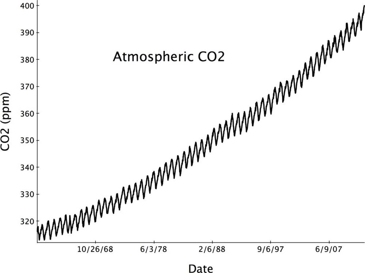
Figure 1-4. Time series data measured frequently over a sufficiently long time interval can reveal regular patterns of variation as well as long-term trends. This curve shows that the level of atmospheric CO₂ is steadily and significantly increasing. See the original data from which this figure was drawn.

Not all time series datasets lead to such surprising and significant discoveries as did the CO₂ data, but time series are extremely useful in revealing interesting patterns and trends in data. Alternatively, a study of time series may show that the parameter being measured is either very steady or varies in very irregular ways. Either way, measurements made as a function of time make these behaviors apparent.

A New Look at Time Series Databases

These examples illustrate how valuable multiple observations made over time can be when stored and analyzed effectively. New methods are appearing for building time series databases that are able to handle very large datasets. For this reason, this book examines how large-scale time series data can best be collected, persisted, and accessed for analysis. It does not focus on methods for analyzing time series, although some of these methods were discussed in our previous book on anomaly detection. Nor is the book report intended as a comprehensive survey of the topic of time series data storage. Instead, we explore some of the fundamental issues connected with new types of time series databases (TSDB) and describe in general how you can use this type of data to advantage. We also give you tips that to make it easier to store and access time series data cost effectively and with excellent performance. Throughout, this book focuses on the practical aspects of time series databases.

Before we explore the details of how to build better time series databases, let’s first look at several modern situations in which large-scale times series are useful.