Time Series Databases: New Ways to Store and Access Data (2014)

Chapter 7. Advanced Topics for Time Series Databases

So far, we have considered how time series can be stored in databases where each time series is easily identified: possibly by name, possibly by a combination of tagged values. The applications of such time series databases are broad and cover many needs.

There are situations, however, where the time series databases that we have described so far fall short. One such situation is where we need to have a sense of location in addition to time. An ordinary time series database makes the assumption that essentially all queries will have results filtered primarily based on time. Put another way, time series databases require to you specify which metric and when the data was recorded. Sometimes, however, we need to include the concept of where. We may want to specify only where and when without specifying which. When we make this change to the queries that we want to use, we move from having a time series database to having a geo-temporal database.

Note that it isn’t the inclusion of locational data into a time series database per se that makes it into a geo-temporal database. Any or all of latitude, longitude, x, y, or z could be included in an ordinary time series database without any problem. As long as we know which time series we want and what time range we want, this locational data is just like any other used to identify the time series. It is the requirement that location data be a primary part of querying the database that makes all the difference.

Suppose, for instance, that we have a large number of data-collecting robots wandering the ocean recording surface temperature (and a few other parameters) at various locations as they move around. A natural query for this data is to retrieve all temperature measurements that have been made within a specified distance of a particular point in the ocean. With an ordinary time series database, however, we are only able to scan by a particular robot for a particular time range, yet we cannot know which time to search for to find the measurements for a robot at a particular location—we don’t have any way to build an efficient query to get the data we need, and it’s not practical to scan the entire database. Also, because the location of each robot changes over time, we cannot store the location in the tags for the entire time series. We can, however, solve this problem by creating a geo-temporal database, and here’s how.

Somewhat surprisingly, it is possible to implement a geo-temporal database using an ordinary time series database together with just a little bit of additional machinery called a geo-index. That is, we can do this if the data we collect and the queries we need to do satisfy a few simple assumptions. This chapter describes these assumptions, gives examples of when these assumptions hold, and describes how to implement this kind of geo-temporal database.

Stationary Data

In the special case where each time series is gathered in a single location that does not change, we do not actually need a geo-temporal database. Since the location doesn’t change, the location does not need to be recorded more than once and can instead be recorded as an attribute of the time series itself, just like any other attribute. This means that querying such a database with a region of interest and a time range involves nothing more than finding the time series that are in the region and then issuing a normal time-based query for those time series.

Wandering Sources

The case of time series whose data source location changes over time is much more interesting than the case where location doesn’t change. The exciting news is that if the data source location changes relatively slowly, such as with the ocean robots, there are a variety of methods to make location searches as efficient as time scans. We describe only one method here.

To start with, we assume that all the locations are on a plane that is divided into squares. For an ocean robot, imagine its path mapped out as a curve, and we’ve covered the map with squares. The robot’s path will pass through some of the squares. Where the path crosses a square is what we call an intersection.

We also assume that consecutive points in a time series are collected near one another geographically because the data sources move slowly with respect to how often they collect data. As data is ingested, we can examine the location data for each time series and mark down in a separate table (the geo-index) exactly when the time series path intersects each square and which squares it intersects. These intersections of time series and squares can be stored and indexed by the ID of the square so that we can search the geo-index using the square and get a list of all intersections with that square. That list of intersections tells us which robots have crossed the square and when they crossed it. We can then use that information to query the time series database portion of our geo-temporal database because we now know which and when.

Figure 7-1 shows how this might work with relatively coarse partitioning of spatial data. Two time series that wander around are shown. If we want to find which time series might intersect the shaded circle and when, we can retrieve intersection information for squares A, B, C, D, E, and F. To get the actual time series data that overlaps with the circle, we will have to scan each segment of the time series to find out if they actually do intersect with the circle, but we only have to scan the segments that overlapped with one of these six squares.

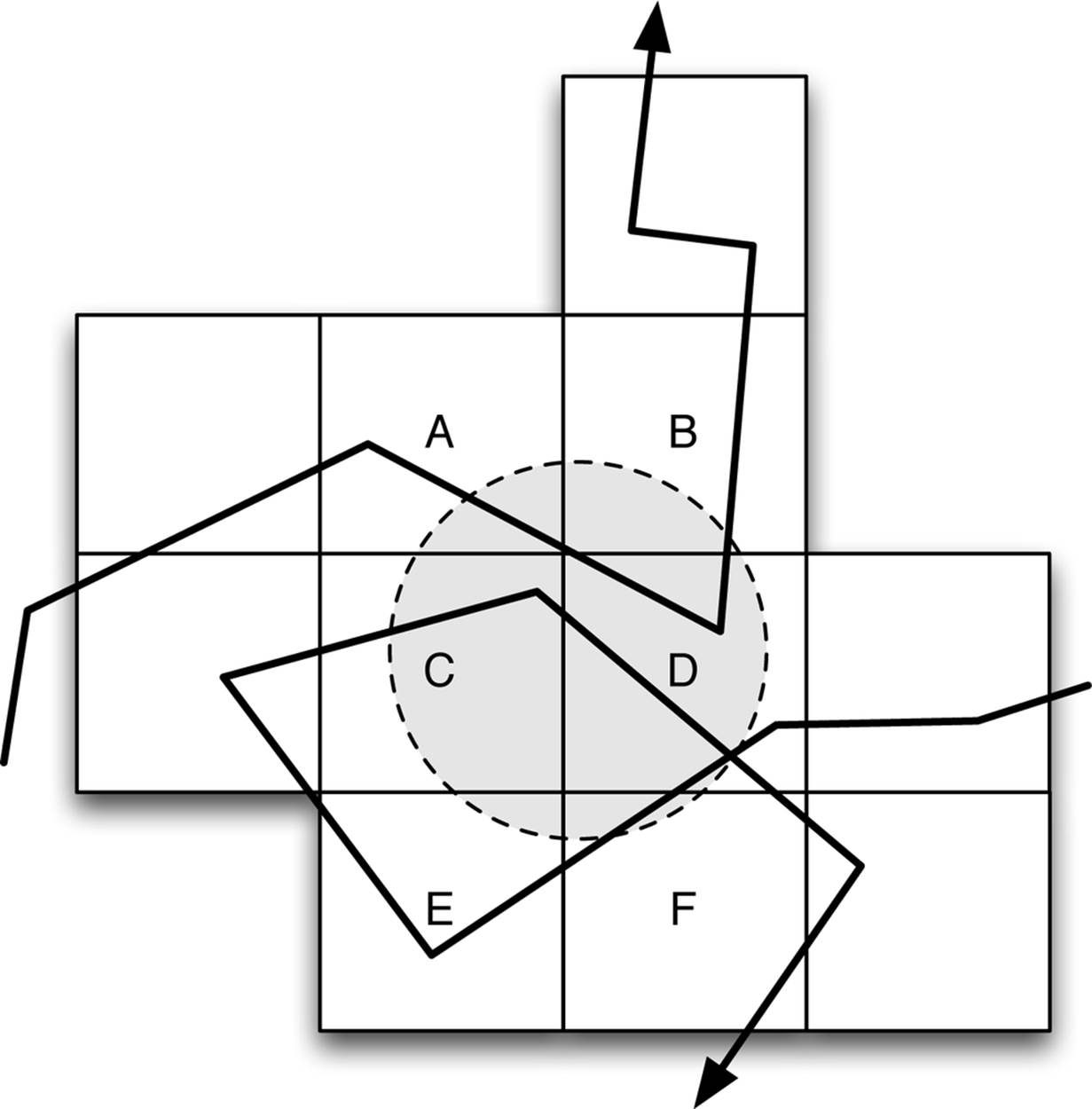
Figure 7-1. To find time windows of series that might intersect with the shaded circle, we only have to check segments that intersect with the six squares A–F. These squares involve considerably more area than we need to search, but in this case, only three segments having no intersection with the circle would have to be scanned because they intersect squares A–F. This means that we need only scan a small part of the total data in the time series database.

If we make the squares smaller like in Figure 7-2, we will have a more precise search that forces us to scan less data that doesn’t actually overlap with the circle. This is good, but as the squares get smaller, the number of data points in the time series during the overlap with each square becomes smaller and smaller. This makes the spatial index bigger and ultimately decreases efficiency.

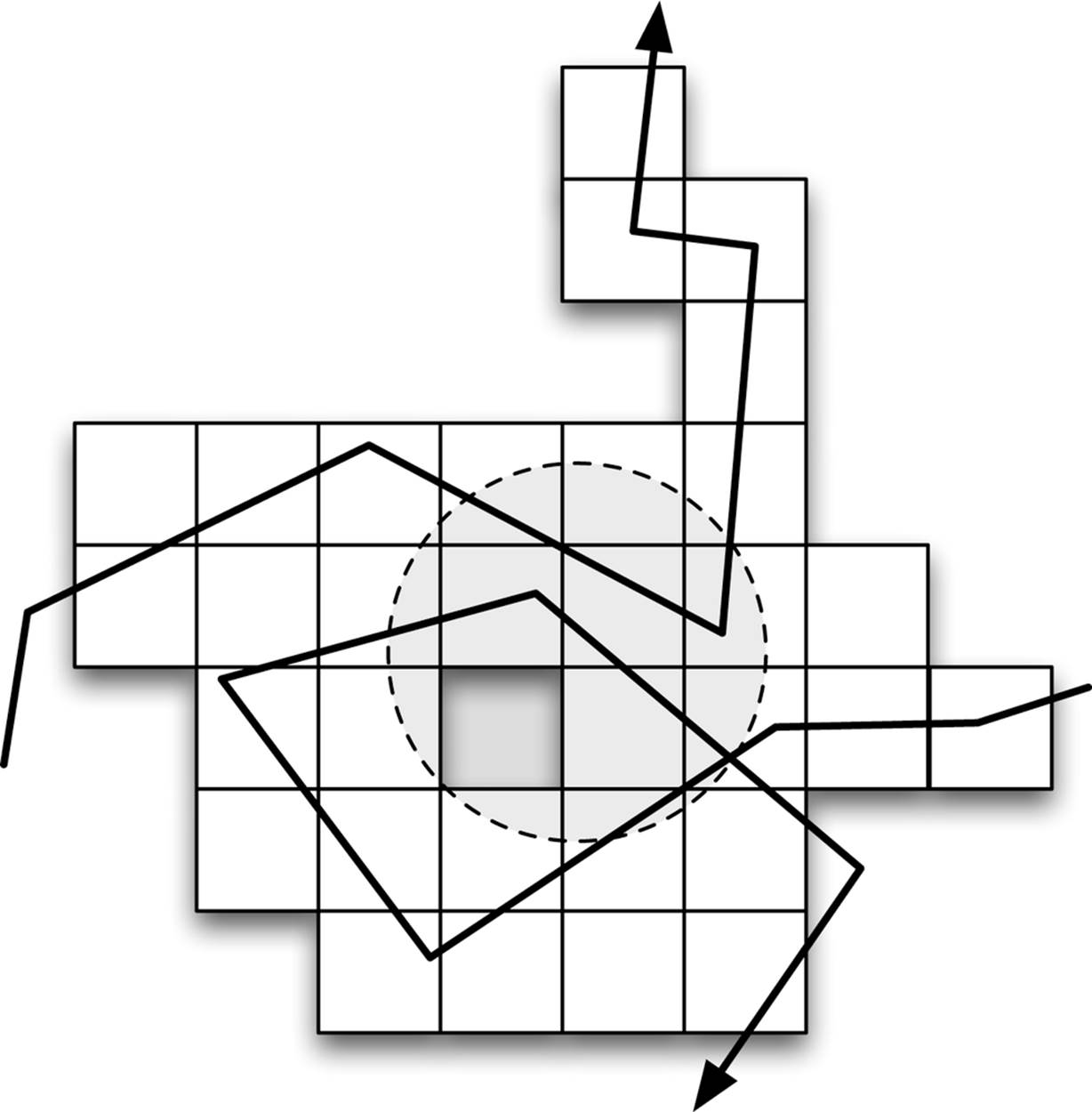
Figure 7-2. With smaller squares, we have more squares to check, but they have an area closer to that of the circle of interest. The circle now intersects 13 squares, but only 2 segments with no intersection will be scanned, and those segments are shorter than before because the squares are smaller.

It is sometimes not possible to find a universal size of square that works well for all of the time series in the database. To avoid that problem, you can create an adaptive spatial index in which intersections are recorded at the smallest scale square possible that still gives enough samples in the time series segment to be efficient. If a time series involves slow motion, a very fine grid will be used. If the time series involves faster motion, a coarser grid will be used. A time series that moves quickly sometimes and more slowly at other times will have a mix of fine and coarse squares. In a database using a blobbed storage format, a good rule of thumb is to record intersections at whichever size square roughly corresponds a single blob of data.

Space-Filling Curves

As a small optimization, you can label the squares in the spatial index according to a pattern known as a Hilbert curve, as shown in Figure 7-3. This labeling is recursively defined so that finer squares share the prefix of their label with overlapping coarser squares. Another nice property of Hilbert labeling is that roughly round or square regions will overlap squares with large runs of sequential labels. This can mean that a database such as Apache HBase that orders items according to their key may need to do fewer disk seeks when finding the content associated with these squares.

Figure 7-3. A square can be recursively divided into quarters and labeled in such a way that the roughly round regions will overlap squares that are nearly contiguous. This ordering can make retrieving the contents associated with each square fast in a database like HBase or MapR-DB because it results in more streaming I/O. This labeling is recursively defined and is closely related to the Hilbert curve.

Whether or not this is an important optimization will depend on how large your geo-index of squares is. Note that Hilbert labeling of squares does not change how the time series themselves are stored, only how the index of squares that is used to find intersections is stored. In many modern systems, the square index will be small enough to fit in memory. If so, Hilbert labeling of the squares will be an unnecessary inconvenience.