Machine Learning with Spark (2015)
Chapter 8. Dimensionality Reduction with Spark
Over the course of this chapter, we will continue our exploration of unsupervised learning models in the form of dimensionality reduction.
Unlike the models we have covered so far, such as regression, classification, and clustering, dimensionality reduction does not focus on making predictions. Instead, it tries to take a set of input data with a feature dimension D (that is, the length of our feature vector) and extract a representation of the data of dimension k, where k is usually significantly smaller than D. It is, therefore, a form of preprocessing or feature transformation rather than a predictive model in its own right.
It is important that the representation that is extracted should still be able to capture a large proportion of the variability or structure of the original data. The idea behind this is that most data sources will contain some form of underlying structure. This structure is typically unknown (often called latent features or latent factors), but if we can uncover some of this structure, our models could learn this structure and make predictions from it rather than from the data in its raw form, which might be noisy or contain many irrelevant features. In other words, dimensionality reduction throws away some of the noise in the data and keeps the hidden structure that is present.
In some cases, the dimensionality of the raw data is far higher than the number of data points we have, so without dimensionality reduction, it would be difficult for other machine learning models, such as classification and regression, to learn anything, as they need to fit a number of parameters that is far larger than the number of training examples (in this sense, these methods bear some similarity to the regularization approaches that we have seen used in classification and regression).
A few use cases of dimensionality reduction techniques include:
· Exploratory data analysis
· Extracting features to train other machine learning models
· Reducing storage and computation requirements for very large models in the prediction phase (for example, a production system that makes predictions)
· Reducing a large group of text documents down to a set of hidden topics or concepts
· Making learning and generalization of models easier when our data has a very large number of features (for example, when working with text, sound, images, or video data, which tends to be very high-dimensional)
In this chapter, we will:
· Introduce the types of dimensionality reduction models available in MLlib
· Work with images of faces to extract features suitable for dimensionality reduction
· Train a dimensionality reduction model using MLlib
· Visualize and evaluate the results
· Perform parameter selection for our dimensionality reduction model
Types of dimensionality reduction
MLlib provides two models for dimensionality reduction; these models are closely related to each other. They are Principal Components Analysis (PCA) and Singular Value Decomposition (SVD).
Principal Components Analysis
PCA operates on a data matrix X and seeks to extract a set of k principal components from X. The principal components are each uncorrelated to each other and are computed such that the first principal component accounts for the largest variation in the input data. Each subsequent principal component is, in turn, computed such that it accounts for the largest variation, provided that it is independent of the principal components computed so far.
In this way, the k principal components returned are guaranteed to account for the highest amount of variation in the input data possible. Each principal component, in fact, has the same feature dimensionality as the original data matrix. Hence, a projection step is required in order to actually perform dimensionality reduction, where the original data is projected into the k-dimensional space represented by the principal components.
Singular Value Decomposition
SVD seeks to decompose a matrix X of dimension m x n into three component matrices:
· U of dimension m x m
· S, a diagonal matrix of size m x n; the entries of S are referred to as the singular values
· VT of dimension n x n
X = U * S * V T
Looking at the preceding formula, it appears that we have not reduced the dimensionality of the problem at all, as by multiplying U, S, and V, we reconstruct the original matrix. In practice, the truncated SVD is usually computed. That is, only the top k singular values, which represent the most variation in the data, are kept, while the rest are discarded. The formula to reconstruct X based on the component matrices is then approximate:
X ~ Uk * Sk * Vk T
An illustration of the truncated SVD is shown here:
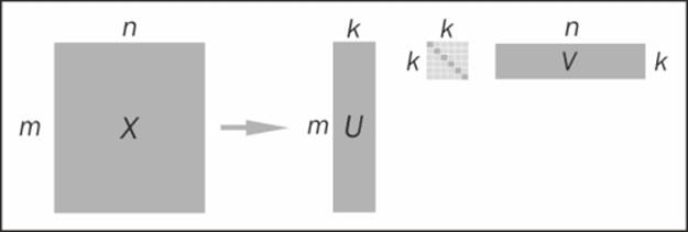
The truncated Singular Value Decomposition
Keeping the top k singular values is similar to keeping the top k principal components in PCA. In fact, SVD and PCA are directly related, as we will see a little later in this chapter.
Note
A detailed mathematical treatment of both PCA and SVD is beyond the scope of this book.
An overview of dimensionality reduction can be found in the Spark documentation at http://spark.apache.org/docs/latest/mllib-dimensionality-reduction.html.
The following links contain a more in-depth mathematical overview of PCA and SVD, respectively: http://en.wikipedia.org/wiki/Principal_component_analysis and http://en.wikipedia.org/wiki/Singular_value_decomposition.
Relationship with matrix factorization
PCA and SVD are both matrix factorization techniques, in the sense that they decompose a data matrix into subcomponent matrices, each of which has a lower dimension (or rank) than the original matrix. Many other dimensionality reduction techniques are based on matrix factorization.
You might remember another example of matrix factorization, that is, collaborative filtering, that we have already seen in Chapter 4, Building a Recommendation Engine with Spark. Matrix factorization approaches to collaborative filtering work by factorizing the ratings matrix into two components: the user factor matrix and the item factor matrix. Each of these has a lower dimension than the original data, so these methods also act as dimensionality reduction models.
Note
Many of the best performing approaches to collaborative filtering include models based on SVD. Simon Funk's approach to the Netflix prize is a famous example. You can look at it at http://sifter.org/~simon/journal/20061211.html.
Clustering as dimensionality reduction
The clustering models we covered in the previous chapter can also be used for a form of dimensionality reduction. This works in the following way:
· Assume that we cluster our high-dimensional feature vectors using a K-means clustering model, with k clusters. The result is a set of k cluster centers.
· We can represent each of our original data points in terms of how far it is from each of these cluster centers. That is, we can compute the distance of a data point to each cluster center. The result is a set of k distances for each data point.
· These k distances can form a new vector of dimension k. We can now represent our original data as a new vector of lower dimension, relative to the original feature dimension.
Depending on the distance metric used, this can result in both dimensionality reduction and a form of nonlinear transformation of the data, allowing us to learn a more complex model while still benefiting from the speed and scalability of a linear model. For example, using a Gaussian or exponential distance function can approximate a very complex nonlinear feature transformation.
Extracting the right features from your data
As with all machine learning models we have explored so far, dimensionality reduction models also operate on a feature vector representation of our data.
For this chapter, we will dive into the world of image processing, using the Labeled Faces in the Wild (LFW) dataset of facial images. This dataset contains over 13,000 images of faces generally taken from the Internet and belonging to well-known public figures. The faces are labeled with the person's name.
Extracting features from the LFW dataset
In order to avoid having to download and process a very large dataset, we will work with a subset of the images, using people who have names that start with an "A". This dataset can be downloaded from http://vis-www.cs.umass.edu/lfw/lfw-a.tgz.
Note
For more details and other variants of the data, visit http://vis-www.cs.umass.edu/lfw/.
The original research paper reference is:
Gary B. Huang, Manu Ramesh, Tamara Berg, and Erik Learned-Miller. Labeled Faces in the Wild: A Database for Studying Face Recognition in Unconstrained Environments. University of Massachusetts, Amherst, Technical Report 07-49, October, 2007.
It can be downloaded from http://vis-www.cs.umass.edu/lfw/lfw.pdf.
Unzip the data using the following command:
>tar xfvz lfw-a.tgz
This will create a folder called lfw, which contains a number of subfolders, one for each person.
Exploring the face data
Start up your Spark Scala console by ensuring that you allocate sufficient memory, as dimensionality reduction methods can be quite computationally expensive:
>./SPARK_HOME/bin/spark-shell --driver-memory 2g
Now that we've unzipped the data, we face a small challenge. Spark provides us with a way to read text files and custom Hadoop input data sources. However, there is no built-in functionality to allow us to read images.
Spark provides a method called wholeTextFiles, which allows us to operate on entire files at once, compared to the textFile method that we have been using so far, which operates on the individual lines within a text file (or multiple files).
We will use the wholeTextFiles method to access the location of each file. Using these file paths, we will write custom code to load and process the images. In the following example code, we will use PATH to refer to the directory in which you extracted the lfwsubdirectory.
We can use a wildcard path specification (using the * character highlighted in the following code snippet) to tell Spark to look in each directory under the lfw directory for files:
val path = "/PATH/lfw/*"
val rdd = sc.wholeTextFiles(path)
val first = rdd.first
println(first)
Running the first command might take a little time, as Spark first scans the specified directory structure for all available files. Once completed, you should see output similar to the one shown here:
first: (String, String) = (file:/PATH/lfw/Aaron_Eckhart/Aaron_Eckhart_0001.jpg,����??JFIF????? ...
You will see that wholeTextFiles returns an RDD that contains key-value pairs, where the key is the file location while the value is the content of the entire text file. For our purposes, we only care about the file path, as we cannot work directly with the image data as a string (notice that it is displayed as "binary nonsense" in the shell output).
Let's extract the file paths from the RDD. Note that earlier, the file path starts with the file: text. This is used by Spark when reading files in order to differentiate between different filesystems (for example, file:// for the local filesystem, hdfs:// for HDFS, s3n:// for Amazon S3, and so on).
In our case, we will be using custom code to read the images, so we don't need this part of the path. Thus, we will remove it with the following map function:
val files = rdd.map { case (fileName, content) => fileName.replace("file:", "") }
println(files.first)
This should display the file location with the file: prefix removed:
/PATH/lfw/Aaron_Eckhart/Aaron_Eckhart_0001.jpg
Next, we will see how many files we are dealing with:
println(files.count)
Running these commands creates a lot of noisy output in the Spark shell, as it outputs all the file paths that are read to the console. Ignore this part, but after the command has completed, the output should look something like this:
..., /PATH/lfw/Azra_Akin/Azra_Akin_0003.jpg:0+19927, /PATH/lfw/Azra_Akin/Azra_Akin_0004.jpg:0+16030
...
14/09/18 20:36:25 INFO SparkContext: Job finished: count at <console>:19, took 1.151955 s
1055
So, we can see that we have 1055 images to work with.
Visualizing the face data
Although there are a few tools available in Scala or Java to display images, this is one area where Python and the matplotlib library shine. We will use Scala to process and extract the images and run our models and IPython to display the actual images.
You can run a separate IPython Notebook by opening a new terminal window and launching a new notebook:
>ipython notebook
Note
Note that if using Python Notebook, you should first execute the following code snippet to ensure that the images are displayed inline after each notebook cell (including the % character): %pylab inline.
Alternatively, you can launch a plain IPython console without the web notebook, enabling the pylab plotting functionality using the following command:
>ipython --pylab
The dimensionality reduction techniques in MLlib are only available in Scala or Java at the time of writing this book, so we will continue to use the Scala Spark shell to run the models. Therefore, you won't need to run a PySpark console.
Tip
We have provided the full Python code with this chapter as a Python script as well as in the IPython Notebook format. For instructions on installing IPython, see the code bundle.
Let's display the image given by the first path we extracted earlier using matplotlib's imread and imshow functions:
path = "/PATH/lfw/PATH/lfw/Aaron_Eckhart/Aaron_Eckhart_0001.jpg"
ae = imread(path)
imshow(ae)
Note
You should see the image displayed in your Notebook (or in a pop-up window if you are using the standard IPython shell). Note that we have not shown the image here.
Extracting facial images as vectors
While a full treatment of image processing is beyond the scope of this book, we will need to know a few basics to proceed. Each color image can be represented as a three-dimensional array, or matrix, of pixels. The first two dimensions, that is the x and y axes, represent the position of each pixel, while the third dimension represents the red, blue, and green (RGB) color values for each pixel.
A grayscale image only requires one value per pixel (there are no RGB values), so it can be represented as a plain two-dimensional matrix. For many image-processing and machine learning tasks related to images, it is common to operate on grayscale images. We will do this here by converting the color images to grayscale first.
It is also a common practice in machine learning tasks to represent an image as a vector, instead of a matrix. We do this by concatenating each row (or alternatively, each column) of the matrix together to form a long vector (this is known as reshaping). In this way, each raw, grayscale image matrix is transformed into a feature vector that is usable as input to a machine learning model.
Fortunately for us, the built-in Java Abstract Window Toolkit (AWT) contains various basic image-processing functions. We will define a few utility functions to perform this processing using the java.awt classes.
Loading images
The first of these is a function to read an image from a file:
import java.awt.image.BufferedImage
def loadImageFromFile(path: String): BufferedImage = {
import javax.imageio.ImageIO
import java.io.File
ImageIO.read(new File(path))
}
This returns an instance of a java.awt.image.BufferedImage class, which stores the image data and provides a number of useful methods. Let's test it out by loading the first image into our Spark shell:
val aePath = "/PATH/lfw/Aaron_Eckhart/Aaron_Eckhart_0001.jpg"
val aeImage = loadImageFromFile(aePath)
You should see the image details displayed in the shell:
aeImage: java.awt.image.BufferedImage = BufferedImage@f41266e: type = 5 ColorModel: #pixelBits = 24 numComponents = 3 color space = java.awt.color.ICC_ColorSpace@7e420794 transparency = 1 has alpha = false isAlphaPre = false ByteInterleavedRaster: width = 250 height = 250 #numDataElements 3 dataOff[0] = 2
There is quite a lot of information here. Of particular interest to us is that the image width and height are 250 pixels, and as we can see, there are three components (that is, the RGB values) that are highlighted in the preceding output.
Converting to grayscale and resizing the images
The next function we will define will take the image that we have loaded with our preceding function, convert the image from color to grayscale, and resize the image's width and height.
These steps are not strictly necessary, but both steps are done in many cases for efficiency purposes. Using RGB color images instead of grayscale increases the amount of data to be processed by a factor of 3. Similarly, larger images increase the processing and storage overhead significantly. Our raw 250 x 250 images represent 187,500 data points per image using three color components. For a set of 1055 images, this is 197,812,500 data points. Even if stored as integer values, each value stored takes 4 bytes of memory, so just 1055 images represent around 800 MB of memory! As you can see, image-processing tasks can quickly become extremely memory intensive.
If we convert to grayscale and resize the images to, say, 50 x 50 pixels, we only require 2500 data points per image. For our 1055 images, this equates to 10 MB of memory, which is far more manageable for illustrative purposes.
Tip
Another reason to resize is that MLlib's PCA model works best on tall and skinny matrices with less than 10,000 columns. We will have 2500 columns (that is, each pixel becomes an entry in our feature vector), so we will come in well below this restriction.
Let's define our processing function. We will do the grayscale conversion and resizing in one step, using the java.awt.image package:
def processImage(image: BufferedImage, width: Int, height: Int): BufferedImage = {
val bwImage = new BufferedImage(width, height, BufferedImage.TYPE_BYTE_GRAY)
val g = bwImage.getGraphics()
g.drawImage(image, 0, 0, width, height, null)
g.dispose()
bwImage
}
The first line of the function creates a new image of the desired width and height and specifies a grayscale color model. The third line draws the original image onto this newly created image. The drawImage method takes care of the color conversion and resizing for us! Finally, we return the new, processed image.
Let's test this out on our sample image. We will convert it to grayscale and resize it to 100 x 100 pixels:
val grayImage = processImage(aeImage, 100, 100)
You should see the following output in the console:
grayImage: java.awt.image.BufferedImage = BufferedImage@21f8ea3b: type = 10 ColorModel: #pixelBits = 8 numComponents = 1 color space = java.awt.color.ICC_ColorSpace@5cd9d8e9 transparency = 1 has alpha = false isAlphaPre = false ByteInterleavedRaster: width = 100 height = 100 #numDataElements 1 dataOff[0] = 0
As you can see from the highlighted output, the image's width and height are indeed 100, and the number of color components is 1.
Next, we will save the processed image to a temporary location so that we can read it back and display it in our IPython console:
import javax.imageio.ImageIO
import java.io.File
ImageIO.write(grayImage, "jpg", new File("/tmp/aeGray.jpg"))
You should see a result of true displayed in your console, indicating that we successfully saved the image to the aeGray.jpg file in our /tmp directory.
Finally, we will read the image in Python and use matplotlib to display the image. Type the following code into your IPython Notebook or shell (remember that this should be open in a new terminal window):
tmpPath = "/tmp/aeGray.jpg"
aeGary = imread(tmpPath)
imshow(aeGary, cmap=plt.cm.gray)
This should display the image (note again, we haven't shown the image here). You should see that it is grayscale and of slightly worse quality as compared to the original image. Furthermore, you will notice that the scale of the axes are different, representing the new 100 x 100 dimension instead of the original 250 x 250 size.
Extracting feature vectors
The final step in the processing pipeline is to extract the actual feature vectors that will be the input to our dimensionality reduction model. As we mentioned earlier, the raw grayscale pixel data will be our features. We will form the vectors by flattening out the two-dimensional pixel matrix. The BufferedImage class provides a utility method to do just this, which we will use in our function:
def getPixelsFromImage(image: BufferedImage): Array[Double] = {
val width = image.getWidth
val height = image.getHeight
val pixels = Array.ofDim[Double](width * height)
image.getData.getPixels(0, 0, width, height, pixels)
}
We can then combine these three functions into one utility function that takes a file location together with the desired image's width and height and returns the raw Array[Double] value that contains the pixel data:
def extractPixels(path: String, width: Int, height: Int): Array[Double] = {
val raw = loadImageFromFile(path)
val processed = processImage(raw, width, height)
getPixelsFromImage(processed)
}
Applying this function to each element of the RDD that contains all the image file paths will give us a new RDD that contains the pixel data for each image. Let's do this and inspect the first few elements:
val pixels = files.map(f => extractPixels(f, 50, 50))
println(pixels.take(10).map(_.take(10).mkString("", ",", ", ...")).mkString("\n"))
You should see output similar to this:
0.0,0.0,0.0,0.0,0.0,0.0,1.0,1.0,0.0,0.0, ...
241.0,243.0,245.0,244.0,231.0,205.0,177.0,160.0,150.0,147.0, ...
253.0,253.0,253.0,253.0,253.0,253.0,254.0,254.0,253.0,253.0, ...
244.0,244.0,243.0,242.0,241.0,240.0,239.0,239.0,237.0,236.0, ...
44.0,47.0,47.0,49.0,62.0,116.0,173.0,223.0,232.0,233.0, ...
0.0,0.0,0.0,0.0,0.0,0.0,0.0,0.0,0.0,0.0, ...
1.0,1.0,1.0,1.0,1.0,1.0,1.0,1.0,0.0,0.0, ...
26.0,26.0,27.0,26.0,24.0,24.0,25.0,26.0,27.0,27.0, ...
240.0,240.0,240.0,240.0,240.0,240.0,240.0,240.0,240.0,240.0, ...
0.0,0.0,0.0,0.0,0.0,0.0,0.0,0.0,0.0,0.0, ...
The final step is to create an MLlib Vector instance for each image. We will cache the RDD to speed up our later computations:
import org.apache.spark.mllib.linalg.Vectors
val vectors = pixels.map(p => Vectors.dense(p))
vectors.setName("image-vectors")
vectors.cache
Tip
We used the setName function earlier to assign an RDD a name. In this case, we called it image-vectors. This is so that we can later identify it more easily when looking at the Spark web interface.
Normalization
It is a common practice to standardize input data prior to running dimensionality reduction models, in particular for PCA. As we did in Chapter 5, Building a Classification Model with Spark, we will do this using the built-in StandardScaler provided by MLlib's featurepackage. We will only subtract the mean from the data in this case:
import org.apache.spark.mllib.linalg.Matrix
import org.apache.spark.mllib.linalg.distributed.RowMatrix
import org.apache.spark.mllib.feature.StandardScaler
val scaler = new StandardScaler(withMean = true, withStd = false).fit(vectors)
Calling fit triggers a computation on our RDD[Vector]. You should see output similar to the one shown here:
...
14/09/21 11:46:58 INFO SparkContext: Job finished: reduce at RDDFunctions.scala:111, took 0.495859 s
scaler: org.apache.spark.mllib.feature.StandardScalerModel = org.apache.spark.mllib.feature.StandardScalerModel@6bb1a1a1
Tip
Note that subtracting the mean works for dense input data. However, for sparse vectors, subtracting the mean vector from each input will transform the sparse data into dense data. For very high-dimensional input, this will likely exhaust the available memory resources, so it is not advisable.
Finally, we will use the returned scaler to transform the raw image vectors to vectors with the column means subtracted:
val scaledVectors = vectors.map(v => scaler.transform(v))
We mentioned earlier that the resized grayscale images would take up around 10 MB of memory. Indeed, you can take a look at the memory usage in the Spark application monitor storage page by going to http://localhost:4040/storage/ in your web browser.
Since we gave our RDD of image vectors a friendly name of image-vectors, you should see something like the following screenshot (note that as we are using Vector[Double], each element takes up 8 bytes instead of 4 bytes; hence, we actually use 20 MB of memory):
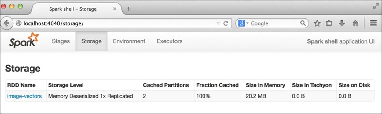
Size of image vectors in memory
Training a dimensionality reduction model
Dimensionality reduction models in MLlib require vectors as inputs. However, unlike clustering that operated on an RDD[Vector], PCA and SVD computations are provided as methods on a distributed RowMatrix (this difference is largely down to syntax, as a RowMatrixis simply a wrapper around an RDD[Vector]).
Running PCA on the LFW dataset
Now that we have extracted our image pixel data into vectors, we can instantiate a new RowMatrix and call the computePrincipalComponents method to compute the top K principal components of our distributed matrix:
import org.apache.spark.mllib.linalg.Matrix
import org.apache.spark.mllib.linalg.distributed.RowMatrix
val matrix = new RowMatrix(scaledVectors)
val K = 10
val pc = matrix.computePrincipalComponents(K)
You will likely see quite a lot of output in your console while the model runs.
Tip
If you see warnings such as WARN LAPACK: Failed to load implementation from: com.github.fommil.netlib.NativeSystemLAPACK or WARN LAPACK: Failed to load implementation from: com.github.fommil.netlib.NativeRefLAPACK, you can safely ignore these.
This means that the underlying linear algebra libraries used by MLlib could not load native routines. In this case, a Java-based fallback will be used, which is slower, but there is nothing to worry about for the purposes of this example.
Once the model training is complete, you should see a result displayed in the console that looks similar to the following one:
pc: org.apache.spark.mllib.linalg.Matrix =
-0.023183157256614906 -0.010622723054037303 ... (10 total)
-0.023960537953442107 -0.011495966728461177 ...
-0.024397470862198022 -0.013512219690177352 ...
-0.02463158818330343 -0.014758658113862178 ...
-0.024941633606137027 -0.014878858729655142 ...
-0.02525998879466241 -0.014602750644394844 ...
-0.025494722450369593 -0.014678013626511024 ...
-0.02604194423255582 -0.01439561589951032 ...
-0.025942214214865228 -0.013907665261197633 ...
-0.026151551334429365 -0.014707035797934148 ...
-0.026106572186134578 -0.016701471378568943 ...
-0.026242986173995755 -0.016254664123732318 ...
-0.02573628754284022 -0.017185663918352894 ...
-0.02545319635905169 -0.01653357295561698 ...
-0.025325893980995124 -0.0157082218373399...
Visualizing the Eigenfaces
Now that we have trained our PCA model, what is the result? Let's inspect the dimensions of the resulting matrix:
val rows = pc.numRows
val cols = pc.numCols
println(rows, cols)
As you should see from your console output, the matrix of principal components has 2500 rows and 10 columns:
(2500,10)
Recall that the dimension of each image is 50 x 50, so here, we have the top 10 principal components, each with a dimension identical to that of the input images. These principal components can be thought of as the set of latent (or hidden) features that capture the greatest variation in the original data.
Note
In facial recognition and image processing, these principal components are often referred to as Eigenfaces, as PCA is closely related to the eigenvalue decomposition of the covariance matrix of the original data.
See http://en.wikipedia.org/wiki/Eigenface for more details.
Since each principal component is of the same dimension as the original images, each component can itself be thought of and represented as an image, making it possible to visualize the Eigenfaces as we would the input images.
As we have often done in this book, we will use functionality from the Breeze linear algebra library as well as Python's numpy and matplotlib to visualize the Eigenfaces.
First, we will extract the pc variable (an MLlib matrix) into a Breeze DenseMatrix:
import breeze.linalg.DenseMatrix
val pcBreeze = new DenseMatrix(rows, cols, pc.toArray)
Breeze provides a useful function within the linalg package to write the matrix out as a CSV file. We will use this to save the principal components to a temporary CSV file:
import breeze.linalg.csvwrite
csvwrite(new File("/tmp/pc.csv"), pcBreeze)
Next, we will load the matrix in IPython and visualize the principal components as images. Fortunately, numpy provides a utility function to read the matrix from the CSV file we created:
pcs = np.loadtxt("/tmp/pc.csv", delimiter=",")
print(pcs.shape)
You should see the following output, confirming that the matrix we read has the same dimensions as the one we saved:
(2500, 10)
We will need a utility function to display the images, which we define here:
def plot_gallery(images, h, w, n_row=2, n_col=5):
"""Helper function to plot a gallery of portraits"""
plt.figure(figsize=(1.8 * n_col, 2.4 * n_row))
plt.subplots_adjust(bottom=0, left=.01, right=.99, top=.90, hspace=.35)
for i in range(n_row * n_col):
plt.subplot(n_row, n_col, i + 1)
plt.imshow(images[:, i].reshape((h, w)), cmap=plt.cm.gray)
plt.title("Eigenface %d" % (i + 1), size=12)
plt.xticks(())
plt.yticks(())
Note
This function is adapted from the LFW dataset example code in the scikit-learn documentation available at http://scikit-learn.org/stable/auto_examples/applications/face_recognition.html.
We will now use this function to plot the top 10 Eigenfaces:
plot_gallery(pcs, 50, 50)
This should display the following plot:
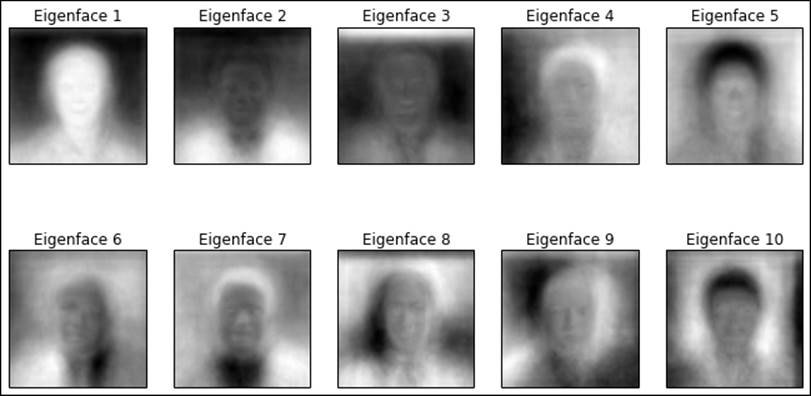
Top 10 Eigenfaces
Interpreting the Eigenfaces
Looking at the preceding images, we can see that the PCA model has effectively extracted recurring patterns of variation, which represent various features of the facial images. Each principal component can, as with clustering models, be interpreted. Again, like clustering, it is not always straightforward to interpret precisely what each principal component represents.
We can see from these images that there appear to be some images that pick up directional factors (for example, images 6 and 9), some hone in on hair patterns (such as images 4, 5, 7, and 10), while others seem to be somewhat more related to facial features such as eyes, nose, and mouth (such as images 1, 7, and 9).
Using a dimensionality reduction model
It is interesting to be able to visualize the outcome of a model in this way; however, the overall purpose of using dimensionality reduction is to create a more compact representation of the data that still captures the important features and variability in the raw dataset. To do this, we need to use a trained model to transform our raw data by projecting it into the new, lower-dimensional space represented by the principal components.
Projecting data using PCA on the LFW dataset
We will illustrate this concept by projecting each LFW image into a ten-dimensional vector. This is done through a matrix multiplication of the image matrix with the matrix of principal components. As the image matrix is a distributed MLlib RowMatrix, Spark takes care of distributing this computation for us through the multiply function:
val projected = matrix.multiply(pc)
println(projected.numRows, projected.numCols)
This will give you the following output:
(1055,10)
Observe that each image that was of dimension 2500 has been transformed into a vector of size 10. Let's take a look at the first few vectors:
println(projected.rows.take(5).mkString("\n"))
Here is the output:
[2648.9455749636277,1340.3713412351376,443.67380716760965,-353.0021423043161,52.53102289832631,423.39861446944354,413.8429065865399,-484.18122999722294,87.98862070273545,-104.62720604921965]
[172.67735747311974,663.9154866829355,261.0575622447282,-711.4857925259682,462.7663154755333,167.3082231097332,-71.44832640530836,624.4911488194524,892.3209964031695,-528.0056327351435]
[-1063.4562028554978,388.3510869550539,1508.2535609357597,361.2485590837186,282.08588829583596,-554.3804376922453,604.6680021092125,-224.16600191143075,-228.0771984153961,-110.21539201855907]
[-4690.549692385103,241.83448841252638,-153.58903325799685,-28.26215061165965,521.8908276360171,-442.0430200747375,-490.1602309367725,-456.78026845649435,-78.79837478503592,70.62925170688868]
[-2766.7960144161225,612.8408888724891,-405.76374113178616,-468.56458995613974,863.1136863614743,-925.0935452709143,69.24586949009642,-777.3348492244131,504.54033662376435,257.0263568009851]
As the projected data is in the form of vectors, we can use the projection as input to another machine learning model. For example, we could use these projected inputs together with a set of input data generated from various images without faces to train a facial recognition model. Alternatively, we could train a multiclass classifier where each person is a class, thus creating a model that learns to identify the particular person that a face belongs to.
The relationship between PCA and SVD
We mentioned earlier that there is a close relationship between PCA and SVD. In fact, we can recover the same principal components and also apply the same projection into the space of principal components using SVD.
In our example, the right singular vectors derived from computing the SVD will be equivalent to the principal components we have calculated. We can see that this is the case by first computing the SVD on our image matrix and comparing the right singular vectors to the result of PCA. As was the case with PCA, SVD computation is provided as a function on a distributed RowMatrix:
val svd = matrix.computeSVD(10, computeU = true)
println(s"U dimension: (${svd.U.numRows}, ${svd.U.numCols})")
println(s"S dimension: (${svd.s.size}, )")
println(s"V dimension: (${svd.V.numRows}, ${svd.V.numCols})")
We can see that SVD returns a matrix U of dimension 1055 x 10, a vector S of the singular values of length 10, and a matrix V of the right singular vectors of dimension 2500 x 10:
U dimension: (1055, 10)
S dimension: (10, )
V dimension: (2500, 10)
The matrix V is exactly equivalent to the result of PCA (ignoring the sign of the values and floating point tolerance). We can verify this with a utility function to compare the two by approximately comparing the data arrays of each matrix:
def approxEqual(array1: Array[Double], array2: Array[Double], tolerance: Double = 1e-6): Boolean = {
// note we ignore sign of the principal component / singular vector elements
val bools = array1.zip(array2).map { case (v1, v2) => if (math.abs(math.abs(v1) - math.abs(v2)) > 1e-6) false else true }
bools.fold(true)(_ & _)
}
We will test the function on some test data:
println(approxEqual(Array(1.0, 2.0, 3.0), Array(1.0, 2.0, 3.0)))
This will give you the following output:
true
Let's try another test data:
println(approxEqual(Array(1.0, 2.0, 3.0), Array(3.0, 2.0, 1.0)))
This will give you the following output:
false
Finally, we can apply our equality function as follows:
println(approxEqual(svd.V.toArray, pc.toArray))
Here is the output:
true
The other relationship that holds is that the multiplication of the matrix U and vector S (or, strictly speaking, the diagonal matrix S) is equivalent to the PCA projection of our original image data into the space of the top 10 principal components.
We will now show that this is indeed the case. We will first use Breeze to multiply each vector in U by S, element-wise. We will then compare each vector in our PCA projected vectors with the equivalent vector in our SVD projection, and sum up the number of equal cases:
val breezeS = breeze.linalg.DenseVector(svd.s.toArray)
val projectedSVD = svd.U.rows.map { v =>
val breezeV = breeze.linalg.DenseVector(v.toArray)
val multV = breezeV :* breezeS
Vectors.dense(multV.data)
}
projected.rows.zip(projectedSVD).map { case (v1, v2) => approxEqual(v1.toArray, v2.toArray) }.filter(b => true).count
This should display a result of 1055, as we would expect, confirming that each row of projected is equal to each row of projectedSVD.
Note
Note that the :* operator highlighted in the preceding code represents element-wise multiplication of the vectors.
Evaluating dimensionality reduction models
Both PCA and SVD are deterministic models. That is, given a certain input dataset, they will always produce the same result. This is in contrast to many of the models we have seen so far, which depend on some random element (most often for the initialization of model weight vectors and so on).
Both models are also guaranteed to return the top principal components or singular values, and hence, the only parameter is k. Like clustering models, increasing k always improves the model performance (for clustering, the relevant error function, while for PCA and SVD, the total amount of variability explained by the k components). Therefore, selecting a value for k is a trade-off between capturing as much structure of the data as possible while keeping the dimensionality of projected data low.
Evaluating k for SVD on the LFW dataset
We will examine the singular values obtained from computing the SVD on our image data. We can verify that the singular values are the same for each run and that they are returned in decreasing order, as follows:
val sValues = (1 to 5).map { i => matrix.computeSVD(i, computeU = false).s }
sValues.foreach(println)
This should show us output similar to the following:
[54091.00997110354]
[54091.00997110358,33757.702867982436]
[54091.00997110357,33757.70286798241,24541.193694775946]
[54091.00997110358,33757.70286798242,24541.19369477593,23309.58418888302]
[54091.00997110358,33757.70286798242,24541.19369477593,23309.584188882982,21803.09841158358]
As with evaluating values of k for clustering, in the case of SVD (and PCA), it is often useful to plot the singular values for a larger range of k and see where the point on the graph is where the amount of additional variance accounted for by each additional singular value starts to flatten out considerably.
We will do this by first computing the top 300 singular values:
val svd300 = matrix.computeSVD(300, computeU = false)
val sMatrix = new DenseMatrix(1, 300, svd300.s.toArray)
csvwrite(new File("/tmp/s.csv"), sMatrix)
We will write out the vector S of singular values to a temporary CSV file (as we did for our matrix of Eigenfaces previously) and then read it back in our IPython console, plotting the singular values for each k:
s = np.loadtxt("/tmp/s.csv", delimiter=",")
print(s.shape)
plot(s)
You should see an image displayed similar to the one shown here:
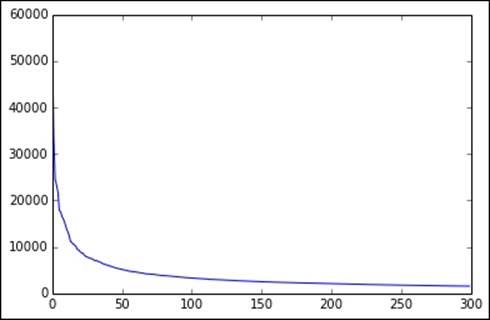
Top 300 singular values
A similar pattern is seen in the cumulative variation accounted for by the top 300 singular values (which we will plot on a log scale for the y axis):
plot(cumsum(s))
plt.yscale('log')
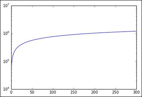
Cumulative sum of top 300 singular values
We can see that after a certain value range for k (around 100 in this case), the graph flattens considerably. This indicates that a number of singular values (or principal components) equivalent to this value of k probably explains enough of the variation of the original data.
Tip
Of course, if we are using dimensionality reduction to help improve the performance of another model, we could use the same evaluation methods used for that model to help us choose a value for k.
For example, we could use the AUC metric, together with cross-validation, to choose both the model parameters for a classification model as well as the value of k for our dimensionality reduction model. This does come at the expense of higher computation cost, however, as we would have to recompute the full model training and testing pipeline.
Summary
In this chapter, we explored two new unsupervised learning methods, PCA and SVD, for dimensionality reduction. We saw how to extract features for and train these models using facial image data. We visualized the results of the model in the form of Eigenfaces, saw how to apply the models to transform our original data into a reduced dimensionality representation, and investigated the close link between PCA and SVD.
In the next chapter, we will delve more deeply into techniques for text processing and analysis with Spark.
All materials on the site are licensed Creative Commons Attribution-Sharealike 3.0 Unported CC BY-SA 3.0 & GNU Free Documentation License (GFDL)
If you are the copyright holder of any material contained on our site and intend to remove it, please contact our site administrator for approval.
© 2016-2026 All site design rights belong to S.Y.A.