Machine Learning with Spark (2015)
Chapter 7. Building a Clustering Model with Spark
In the last few chapters, we covered supervised learning methods, where the training data is labeled with the true outcome that we would like to predict (for example, a rating for recommendations and class assignment for classification or real target variable in the case of regression).
Next, we will consider the case when we do not have labeled data available. This is called unsupervised learning, as the model is not supervised with the true target label. The unsupervised case is very common in practice, since obtaining labeled training data can be very difficult or expensive in many real-world scenarios (for example, having humans label training data with class labels for classification). However, we would still like to learn some underlying structure in the data and use these to make predictions.
This is where unsupervised learning approaches can be useful. Unsupervised learning models are also often combined with supervised models, for example, applying unsupervised techniques to create new input features for supervised models.
Clustering models are, in many ways, the unsupervised equivalent of classification models. With classification, we tried to learn a model that would predict which class a given training example belonged to. The model was essentially a mapping from a set of features to the class.
In clustering, we would like to segment the data such that each training example is assigned to a segment called a cluster. The clusters act much like classes, except that the true class assignments are unknown.
Clustering models have many use cases that are the same as classification; these include the following:
· Segmenting users or customers into different groups based on behavior characteristics and metadata
· Grouping content on a website or products in a retail business
· Finding clusters of similar genes
· Segmenting communities in ecology
· Creating image segments for use in image analysis applications such as object detection
In this chapter, we will:
· Briefly explore a few types of clustering models
· Extract features from data specifically using the output of one model as input features for our clustering model
· Train a clustering model and use it to make predictions
· Apply performance-evaluation and parameter-selection techniques to select the optimal number of clusters to use
Types of clustering models
There are many different forms of clustering models available, ranging from simple to extremely complex ones. The MLlib library currently provides K-means clustering, which is among the simplest approaches available. However, it is often very effective, and its simplicity means it is relatively easy to understand and is scalable.
K-means clustering
K-means attempts to partition a set of data points into K distinct clusters (where K is an input parameter for the model).
More formally, K-means tries to find clusters so as to minimize the sum of squared errors (or distances) within each cluster. This objective function is known as the within cluster sum of squared errors (WCSS).
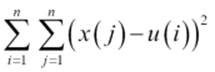
It is the sum, over each cluster, of the squared errors between each point and the cluster center.
Starting with a set of K initial cluster centers (which are computed as the mean vector for all data points in the cluster), the standard method for K-means iterates between two steps:
1. Assign each data point to the cluster that minimizes the WCSS. The sum of squares is equivalent to the squared Euclidean distance; therefore, this equates to assigning each point to the closest cluster center as measured by the Euclidean distance metric.
2. Compute the new cluster centers based on the cluster assignments from the first step.
The algorithm proceeds until either a maximum number of iterations has been reached or convergence has been achieved. Convergence means that the cluster assignments no longer change during the first step; therefore, the value of the WCSS objective function does not change either.
Tip
For more details, refer to Spark's documentation on clustering at http://spark.apache.org/docs/latest/mllib-clustering.html or refer to http://en.wikipedia.org/wiki/K-means_clustering.
To illustrate the basics of K-means, we will use the simple dataset we showed in our multiclass classification example in Chapter 5, Building a Classification Model with Spark. Recall that we have five classes, which are shown in the following figure:
Multiclass dataset
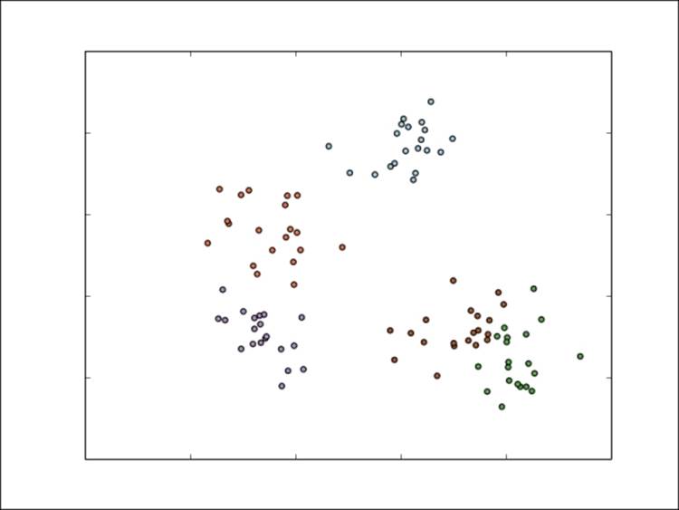
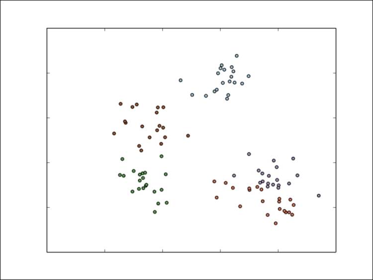
However, assume that we don't actually know the true classes. If we use K-means with five clusters, then after the first step, the model's cluster assignments might look like this:
Cluster assignments after the first K-means iteration
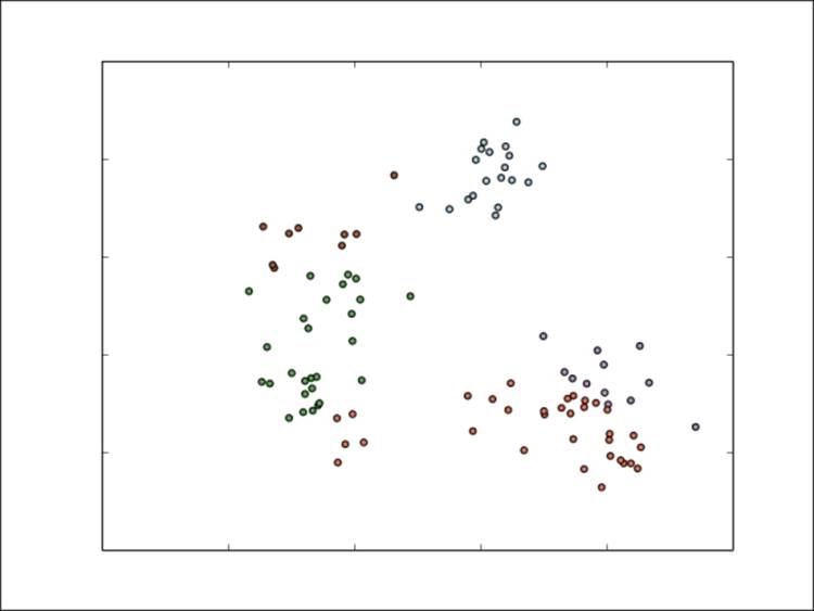
We can see that K-means has already picked out the centers of each cluster fairly well. After the next iteration, the assignments might look like those shown in the following figure:
Cluster assignments after the second K-means iteration
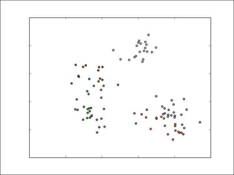
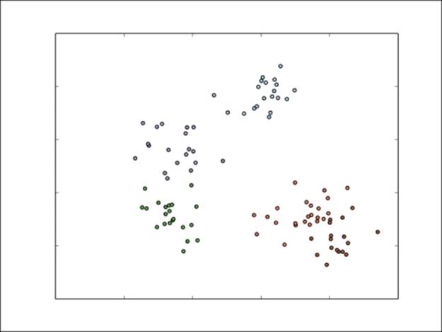
Things are starting to stabilize, but the overall cluster assignments are broadly the same as they were after the first iteration. Once the model has converged, the final assignments could look like this:
Final cluster assignments for K-means
As we can see, the model has done a decent job of separating the five clusters. The leftmost three are fairly accurate (with a few incorrect points). However, the two clusters in the bottom-right corner are less accurate.
This illustrates:
· The iterative nature of K-means
· The model's dependency on the method of initially selecting clusters' centers (here, we will use a random approach)
· That the final cluster assignments can be very good for well-separated data but can be poor for data that is more difficult
Initialization methods
The standard initialization method for K-means, usually simply referred to as the random method, starts by randomly assigning each data point to a cluster before proceeding with the first update step.
MLlib provides a parallel variant for this initialization method, called K-means ||, which is the default initialization method used.
MLlib provides a parallel variant called K-means ||, ||, for this initialization method; this is the default initialization method used.
Note
See http://en.wikipedia.org/wiki/K-means_clustering#Initialization_methods and http://en.wikipedia.org/wiki/K-means%2B%2B for more information.
The results of using K-means++ are shown here. Note that this time, the difficult lower-right points have been mostly correctly clustered.
Final cluster assignments for K-means++
Variants
There are many other variants of K-means; they focus on initialization methods or the core model. One of the more common variants is fuzzy K-means. This model does not assign each point to one cluster as K-means does (a so-called hard assignment). Instead, it is a soft version of K-means, where each point can belong to many clusters, and is represented by the relative membership to each cluster. So, for K clusters, each point is represented as a K-dimensional membership vector, with each entry in this vector indicating the membership proportion in each cluster.
Mixture models
A mixture model is essentially an extension of the idea behind fuzzy K-means; however, it makes an assumption that there is an underlying probability distribution that generates the data. For example, we might assume that the data points are drawn from a set of K-independent Gaussian (normal) probability distributions. The cluster assignments are also soft, so each point is represented by K membership weights in each of the K underlying probability distributions.
Note
See http://en.wikipedia.org/wiki/Mixture_model for further details and for a mathematical treatment of mixture models.
Hierarchical clustering
Hierarchical clustering is a structured clustering approach that results in a multilevel hierarchy of clusters, where each cluster might contain many subclusters (or child clusters). Each child cluster is, thus, linked to the parent cluster. This form of clustering is often also called tree clustering.
Agglomerative clustering is a bottom-up approach where:
· Each data point begins in its own cluster
· The similarity (or distance) between each pair of clusters is evaluated
· The pair of clusters that are most similar are found; this pair is then merged to form a new cluster
· The process is repeated until only one top-level cluster remains
Divisive clustering is a top-down approach that works in reverse, starting with one cluster and at each stage, splitting a cluster into two, until all data points are allocated to their own bottom-level cluster.
Note
You can find more information at http://en.wikipedia.org/wiki/Hierarchical_clustering.
Extracting the right features from your data
Like most of the machine learning models we have encountered so far, K-means clustering requires numerical vectors as input. The same feature extraction and transformation approaches that we have seen for classification and regression are applicable for clustering.
As K-means, like least squares regression, uses a squared error function as the optimization objective, it tends to be impacted by outliers and features with large variance.
As for regression and classification cases, input data can be normalized and standardized to overcome this, which might improve accuracy. In some cases, however, it might be desirable not to standardize data, if, for example, the objective is to find segmentations according to certain specific features.
Extracting features from the MovieLens dataset
For this example, we will return to the movie rating dataset we used in Chapter 4, Building a Recommendation Engine with Spark. Recall that we have three main datasets: one that contains the movie ratings (in the u.data file), a second one with user data (u.user), and a third one with movie data (u.item). We will also be using the genre data file to extract the genres for each movie (u.genre).
We will start by looking at the movie data:
val movies = sc.textFile("/PATH/ml-100k/u.item")
println(movies.first)
This should output the first line of the dataset:
1|Toy Story (1995)|01-Jan-1995||http://us.imdb.com/M/title-exact?Toy%20Story%20(1995)|0|0|0|1|1|1|0|0|0|0|0|0|0|0|0|0|0|0|0
So, we have access to the move title, and we already have the movies categorized into genres. Why do we need to apply a clustering model to the movies? Clustering the movies is a useful exercise for two reasons:
· First, because we have access to the true genre labels, we can use these to evaluate the quality of the clusters that the model finds
· Second, we might wish to segment the movies based on some other attributes or features, apart from their genres
For example, in this case, it seems that we don't have a lot of data to use for clustering, apart from the genres and title. However, this is not true—we also have the ratings data. Previously, we created a matrix factorization model from the ratings data. The model is made up of a set of user and movie factor vectors.
We can think of the movie factors as representing each movie in a new latent feature space, where each latent feature, in turn, represents some form of structure in the ratings matrix. While it is not possible to directly interpret each latent feature, they might represent some hidden structure that influences the ratings behavior between users and movies. One factor could represent genre preference, another could refer to actors or directors, while yet another could represent the theme of the movie, and so on.
So, if we use these factor vector representations of each movie as inputs to our clustering model, we will end up with a clustering that is based on the actual rating behavior of users rather than manual genre assignments.
The same logic applies to the user factors—they represent users in the latent feature space of rating behavior, so clustering the user vectors should result in a clustering based on user rating behavior.
Extracting movie genre labels
Before proceeding further, let's extract the genre mappings from the u.genre file. As you can see from the first line of the preceding dataset, we will need to map from the numerical genre assignments to the textual version so that they are readable.
Take a look at the first few lines of u.genre:
val genres = sc.textFile("/PATH/ml-100k/u.genre")
genres.take(5).foreach(println)
You should see the following output displayed:
unknown|0
Action|1
Adventure|2
Animation|3
Children's|4
Here, 0 is the index of the relevant genre, while unknown is the genre assigned for this index. The indices correspond to the indices of the binary subvector that will represent the genres for each movie (that is, the 0s and 1s in the preceding movie data).
To extract the genre mappings, we will split each line and extract a key-value pair, where the key is the text genre and the value is the index. Note that we have to filter out an empty line at the end; this will, otherwise, throw an error when we try to split the line (see the code highlighted here):
val genreMap = genres.filter(!_.isEmpty).map(line => line.split("\\|")).map(array => (array(1), array(0))).collectAsMap
println(genreMap)
The preceding code will provide the following output:
Map(2 -> Adventure, 5 -> Comedy, 12 -> Musical, 15 -> Sci-Fi, 8 -> Drama, 18 -> Western, ...
Next, we'll create a new RDD from the movie data and our genre mapping; this RDD contains the movie ID, title, and genres. We will use this later to create a more readable output when we evaluate the clusters assigned to each movie by our clustering model.
In the following code section, we will map over each movie and extract the genres subvector (which will still contain Strings rather than Int indexes). We will then apply the zipWithIndex method to create a new collection that contains the indices of the genre subvector, and we will filter this collection so that we are left only with the positive assignments (that is, the 1s that denote a genre assignment for the relevant index). We can then use our extracted genre mapping to map these indices to the textual genres. Finally, we will inspect the first record of the new RDD to see the result of these operations:
val titlesAndGenres = movies.map(_.split("\\|")).map { array =>
val genres = array.toSeq.slice(5, array.size)
val genresAssigned = genres.zipWithIndex.filter { case (g, idx) =>
g == "1"
}.map { case (g, idx) =>
genreMap(idx.toString)
}
(array(0).toInt, (array(1), genresAssigned))
}
println(titlesAndGenres.first)
This should output the following result:
(1,(Toy Story (1995),ArrayBuffer(Animation, Children's, Comedy)))
Training the recommendation model
To get the user and movie factor vectors, we first need to train another recommendation model. Fortunately, we have already done this in Chapter 4, Building a Recommendation Engine with Spark, so we will follow the same procedure:
import org.apache.spark.mllib.recommendation.ALS
import org.apache.spark.mllib.recommendation.Rating
val rawData = sc.textFile("/PATH/ml-100k/u.data")
val rawRatings = rawData.map(_.split("\t").take(3))
val ratings = rawRatings.map{ case Array(user, movie, rating) => Rating(user.toInt, movie.toInt, rating.toDouble) }
ratings.cache
val alsModel = ALS.train(ratings, 50, 10, 0.1)
Recall from Chapter 4, Building a Recommendation Engine with Spark, that the ALS model returned contains the factors in two RDDs of key-value pairs (called userFeatures and productFeatures) with the user or movie ID as the key and the factor as the value. We will need to extract just the factors and transform each one of them into an MLlib Vector to use as training input for our clustering model.
We will do this for both users and movies as follows:
import org.apache.spark.mllib.linalg.Vectors
val movieFactors = alsModel.productFeatures.map { case (id, factor) => (id, Vectors.dense(factor)) }
val movieVectors = movieFactors.map(_._2)
val userFactors = alsModel.userFeatures.map { case (id, factor) => (id, Vectors.dense(factor)) }
val userVectors = userFactors.map(_._2)
Normalization
Before we train our clustering model, it might be useful to look into the distribution of the input data in the form of the factor vectors. This will tell us whether we need to normalize the training data.
We will follow the same approach as we did in Chapter 5, Building a Classification Model with Spark, using MLlib's summary statistics available in the distributed RowMatrix class:
import org.apache.spark.mllib.linalg.distributed.RowMatrix
val movieMatrix = new RowMatrix(movieVectors)
val movieMatrixSummary = movieMatrix.computeColumnSummaryStatistics()
val userMatrix = new RowMatrix(userVectors)
val userMatrixSummary =
userMatrix.computeColumnSummaryStatistics()
println("Movie factors mean: " + movieMatrixSummary.mean)
println("Movie factors variance: " + movieMatrixSummary.variance)
println("User factors mean: " + userMatrixSummary.mean)
println("User factors variance: " + userMatrixSummary.variance)
You should see output similar to the one here:
Movie factors mean: [0.28047737659519767,0.26886479057520024,0.2935579964446398,0.27821738264113755, ...
Movie factors variance: [0.038242041794064895,0.03742229118854288,0.044116961097355877,0.057116244055791986, ...
User factors mean: [0.2043520841572601,0.22135773814655782,0.2149706318418221,0.23647602029329481, ...
User factors variance: [0.037749421148850396,0.02831191551960241,0.032831876953314174,0.036775110657850954, ...
If we look at the output, we will see that there do not appear to be any important outliers that might skew the clustering results, so normalization should not be required in this case.
Training a clustering model
Training for K-means in MLlib takes an approach similar to the other models—we pass an RDD that contains our training data to the train method of the KMeans object. Note that here we do not use LabeledPoint instances, as the labels are not used in clustering; they are used only in the feature vectors. Thus, we use a RDD [Vector] as input to the train method.
Training a clustering model on the MovieLens dataset
We will train a model for both the movie and user factors that we generated by running our recommendation model. We need to pass in the number of clusters K and the maximum number of iterations for the algorithm to run. Model training might run for less than the maximum number of iterations if the change in the objective function from one iteration to the next is less than the tolerance level (the default for this tolerance is 0.0001).
MLlib's K-means provides random and K-means || initialization, with the default being K-means ||. As both of these initialization methods are based on random selection to some extent, each model training run will return a different result.
K-means does not generally converge to a global optimum model, so performing multiple training runs and selecting the most optimal model from these runs is a common practice. MLlib's training methods expose an option to complete multiple model training runs. The best training run, as measured by the evaluation of the loss function, is selected as the final model.
We will first set up the required imports, as well as model parameters: K, maximum iterations, and number of runs:
import org.apache.spark.mllib.clustering.KMeans
val numClusters = 5
val numIterations = 10
val numRuns = 3
We will then run K-means on the movie factor vectors:
val movieClusterModel = KMeans.train(movieVectors, numClusters, numIterations, numRuns)
Once the model has completed training, we should see output that looks something like this:
...
14/09/02 21:53:58 INFO SparkContext: Job finished: collectAsMap at KMeans.scala:193, took 0.02043 s
14/09/02 21:53:58 INFO KMeans: Iterations took 0.331 seconds.
14/09/02 21:53:58 INFO KMeans: KMeans reached the max number of iterations: 10.
14/09/02 21:53:58 INFO KMeans: The cost for the best run is 2586.298785925147
.
...
movieClusterModel: org.apache.spark.mllib.clustering.KMeansModel = org.apache.spark.mllib.clustering.KMeansModel@71c6f512
As can be seen from the highlighted text, the model training output tells us that the maximum number of iterations was reached, so the training process did not stop early based on the convergence criterion. It also shows the training set error (that is, the value of the K-means objective function) for the best run.
We can try a much larger setting for the maximum iterations and use only one training run to see an example where the K-means model converges:
val movieClusterModelConverged = KMeans.train(movieVectors, numClusters, 100)
You should be able to see the KMeans converged in ... iterations text in the model output; this text indicates that after so many iterations, the K-means objective function did not decrease more than the tolerance level:
...
14/09/02 22:04:38 INFO SparkContext: Job finished: collectAsMap at KMeans.scala:193, took 0.040685 s
14/09/02 22:04:38 INFO KMeans: Run 0 finished in 34 iterations
14/09/02 22:04:38 INFO KMeans: Iterations took 0.812 seconds.
14/09/02 22:04:38 INFO KMeans: KMeans converged in 34 iterations.
14/09/02 22:04:38 INFO KMeans: The cost for the best run is 2584.9354332904104.
...
movieClusterModelConverged: org.apache.spark.mllib.clustering.KMeansModel = org.apache.spark.mllib.clustering.KMeansModel@6bb28fb5
Tip
Notice that when we use a lower number of iterations but use multiple training runs, we typically get a training error (called cost above) that is very similar to the one we obtain by running the model to convergence. Using the multiple runs option can, therefore, be a very effective method to find the best possible model.
Finally, we will also train a K-means model on the user factor vectors:
val userClusterModel = KMeans.train(userVectors, numClusters, numIterations, numRuns)
Making predictions using a clustering model
Using the trained K-means model is straightforward and similar to the other models we have encountered so far, such as classification and regression. We can make a prediction for a single Vector instance as follows:
val movie1 = movieVectors.first
val movieCluster = movieClusterModel.predict(movie1)
println(movieCluster)
We can also make predictions for multiple inputs by passing a RDD [Vector] to the predict method of the model:
val predictions = movieClusterModel.predict(movieVectors)
println(predictions.take(10).mkString(","))
The resulting output is a cluster assignment for each data point:
0,0,1,1,2,1,0,1,1,1
Tip
Note that due to random initialization, the cluster assignments might change from one run of the model to another, so your results might differ from those shown earlier. The cluster ID themselves have no inherent meaning; they are simply arbitrarily labeled, starting from 0.
Interpreting cluster predictions on the MovieLens dataset
We have covered how to make predictions for a set of input vectors, but how do we evaluate how good the predictions are? We will cover performance metrics a little later; however, here, we will see how to manually inspect and interpret the cluster assignments made by our K-means model.
While unsupervised techniques have the advantage that they do not require us to provide labeled data for training, the disadvantage is that often, the results need to be manually interpreted. Often, we would like to further examine the clusters that are found and possibly try to interpret them and assign some sort of labeling or categorization to them.
For example, we can examine the clustering of movies we have found to try to see whether there is some meaningful interpretation of each cluster, such as a common genre or theme among the movies in the cluster. There are many approaches we can use, but we will start by taking a few movies in each cluster that are closest to the center of the cluster. These movies, we assume, would be the ones that are least likely to be marginal in terms of their cluster assignment, and so, they should be among the most representative of the movies in the cluster. By examining these sets of movies, we can see what attributes are shared by the movies in each cluster.
Interpreting the movie clusters
To begin, we need to decide what we mean by "closest to the center of each cluster". The objective function that is minimized by K-means is the sum of Euclidean distances between each point and the cluster center, summed over all clusters. Therefore, it is natural to use the Euclidean distance as our measure.
We will define this function here. Note that we will need access to certain imports from the Breeze library (a dependency of MLlib) for linear algebra and vector-based numerical functions:
import breeze.linalg._
import breeze.numerics.pow
def computeDistance(v1: DenseVector[Double], v2: DenseVector[Double]) = pow(v1 - v2, 2).sum
Tip
The preceding pow function is a Breeze universal function. This function is the same as the pow function from scala.math, except that it operates element-wise on the vector that is returned from the minus operation between the two input vectors.
Now, we will use this function to compute, for each movie, the distance of the relevant movie factor vector from the center vector of the assigned cluster. We will also join our cluster assignments and distances data with the movie titles and genres so that we can output the results in a more readable way:
val titlesWithFactors = titlesAndGenres.join(movieFactors)
val moviesAssigned = titlesWithFactors.map { case (id, ((title, genres), vector)) =>
val pred = movieClusterModel.predict(vector)
val clusterCentre = movieClusterModel.clusterCenters(pred)
val dist = computeDistance(DenseVector(clusterCentre.toArray), DenseVector(vector.toArray))
(id, title, genres.mkString(" "), pred, dist)
}
val clusterAssignments = moviesAssigned.groupBy { case (id, title, genres, cluster, dist) => cluster }.collectAsMap
After running the preceding code snippet, we have an RDD that contains a set of key-value pairs for each cluster; here, the key is the numeric cluster identifier, and the value is made up of a set of movies and related information. The movie information we have is the movie ID, title, genres, cluster index, and distance of the movie's factor vector from the cluster center.
Finally, we will iterate through each cluster and output the top 20 movies, ranked by distance from closest to the cluster center:
for ( (k, v) <- clusterAssignments.toSeq.sortBy(_._1)) {
println(s"Cluster $k:")
val m = v.toSeq.sortBy(_._5)
println(m.take(20).map { case (_, title, genres, _, d) => (title, genres, d) }.mkString("\n"))
println("=====\n")
}
The following screenshot is an example output. Note that your output might differ due to random initializations of both the recommendation and clustering model.
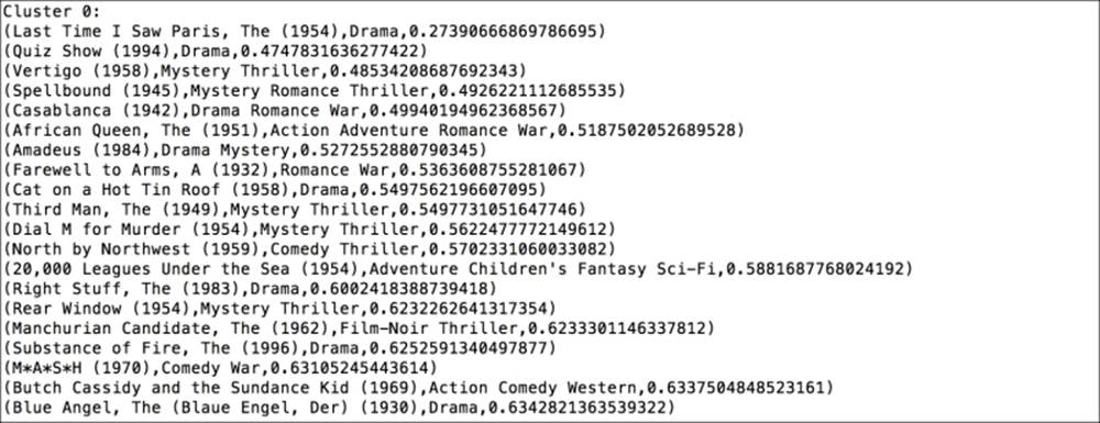
The first cluster
The first cluster, labeled 0, seems to contain a lot of old movies from the 1940s, 1950s, and 1960s, as well as a scattering of recent dramas.
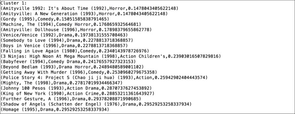
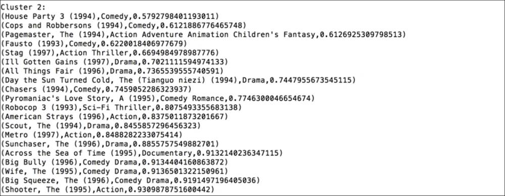
The second cluster
The second cluster has a few horror movies in a prominent position, while the rest of the movies are less clear, but dramas are common too.
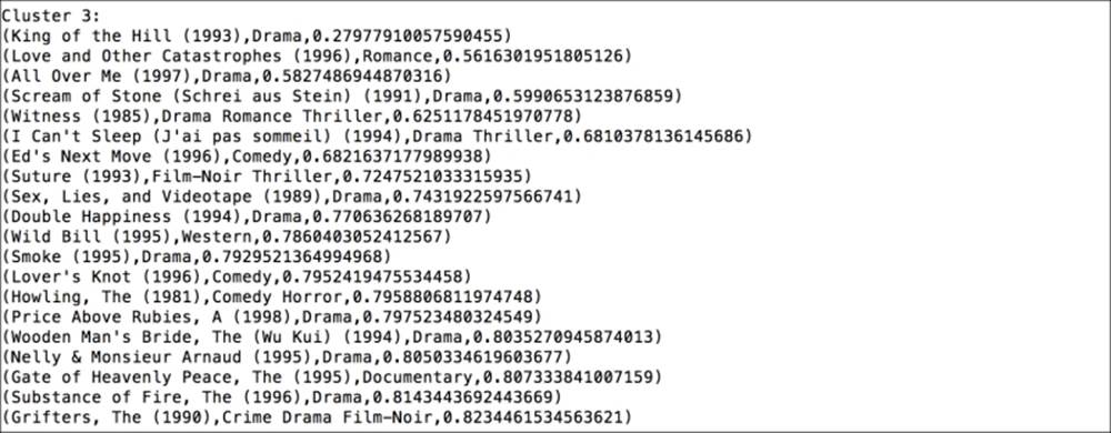
The third cluster
The third cluster is not clear-cut but has a fair number of comedy and drama movies.
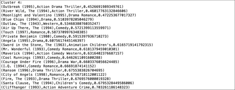
The fourth cluster
The next cluster is more clearly associated with dramas and contains some foreign language films in particular.
The last cluster
The final cluster seems to be related predominantly to action and thrillers as well as romance movies, and seems to contain a number of relatively popular movies.
As you can see, it is not always straightforward to determine exactly what each cluster represents. However, there is some evidence here that the clustering is picking out attributes or commonalities between groups of movies, which might not be immediately obvious based only on the movie titles and genres (such as a foreign language segment, a classic movie segment, and so on). If we had more metadata available, such as directors, actors, and so on, we might find out more details about the defining features of each cluster.
Tip
We leave it as an exercise for you to perform a similar investigation into the clustering of the user factors. We have already created the input vectors in the userVectors variable, so you can train a K-means model on these vectors. After that, in order to evaluate the clusters, you would need to investigate the closest users for each cluster center (as we did for movies) and see if some common characteristics can be identified from the movies they have rated or the user metadata available.
Evaluating the performance of clustering models
Like models such as regression, classification, and recommendation engines, there are many evaluation metrics that can be applied to clustering models to analyze their performance and the goodness of the clustering of the data points. Clustering evaluation is generally divided into either internal or external evaluation. Internal evaluation refers to the case where the same data used to train the model is used for evaluation. External evaluation refers to using data external to the training data for evaluation purposes.
Internal evaluation metrics
Common internal evaluation metrics include the WCSS we covered earlier (which is exactly the K-means objective function), the Davies-Bouldin index, the Dunn Index, and the silhouette coefficient. All these measures tend to reward clusters where elements within a cluster are relatively close together, while elements in different clusters are relatively far away from each other.
Note
The Wikipedia page on clustering evaluation at http://en.wikipedia.org/wiki/Cluster_analysis#Internal_evaluation has more details.
External evaluation metrics
Since clustering can be thought of as unsupervised classification, if we have some form of labeled (or partially labeled) data available, we could use these labels to evaluate a clustering model. We can make predictions of clusters (that is, the class labels) using the model and evaluate the predictions against the true labels using metrics similar to some that we saw for classification evaluation (that is, based on true positive and negative and false positive and negative rates).
These include the Rand measure, F-measure, Jaccard index, and others.
Note
See http://en.wikipedia.org/wiki/Cluster_analysis#External_evaluation for more information on external evaluation for clustering.
Computing performance metrics on the MovieLens dataset
MLlib provides a convenient computeCost function to compute the WCSS objective function given a RDD [Vector]. We will compute this metric for the following movie and user training data:
val movieCost = movieClusterModel.computeCost(movieVectors)
val userCost = userClusterModel.computeCost(userVectors)
println("WCSS for movies: " + movieCost)
println("WCSS for users: " + userCost)
This should output the result similar to the following one:
WCSS for movies: 2586.0777166339426
WCSS for users: 1403.4137493396831
Tuning parameters for clustering models
In contrast to many of the other models we have come across so far, K-means only has one parameter that can be tuned. This is K, the number of cluster centers chosen.
Selecting K through cross-validation
As we have done with classification and regression models, we can apply cross-validation techniques to select the optimal number of clusters for our model. This works in much the same way as for supervised learning methods. We will split the dataset into a training set and a test set. We will then train a model on the training set and compute the evaluation metric of interest on the test set.
We will do this for the movie clustering using the built-in WCSS evaluation metric provided by MLlib in the following code, using a 60 percent / 40 percent split between the training set and test set:
val trainTestSplitMovies = movieVectors.randomSplit(Array(0.6, 0.4), 123)
val trainMovies = trainTestSplitMovies(0)
val testMovies = trainTestSplitMovies(1)
val costsMovies = Seq(2, 3, 4, 5, 10, 20).map { k => (k, KMeans.train(trainMovies, numIterations, k, numRuns).computeCost(testMovies)) }
println("Movie clustering cross-validation:")
costsMovies.foreach { case (k, cost) => println(f"WCSS for K=$k id $cost%2.2f") }
This should give results that look something like the ones shown here.
The output of movie clustering cross-validation is:
Movie clustering cross-validation
WCSS for K=2 id 942.06
WCSS for K=3 id 942.67
WCSS for K=4 id 950.35
WCSS for K=5 id 948.20
WCSS for K=10 id 943.26
WCSS for K=20 id 947.10
We can observe that the WCSS decreases as the number of clusters increases, up to a point. It then begins to increase. Another common pattern observed in the WCSS in cross-validation for K-means is that the metric continues to decrease as K increases, but at a certain point, the rate of decrease flattens out substantially. The value of K at which this occurs is generally selected as the optimal K parameter (this is sometimes called the elbow point, as this is where the line kinks when drawn as a graph).
In our case, we might select a value of 10 for K, based on the preceding results. Also, note that the clusters that are computed by the model are often used for purposes that require some human interpretation (such as the cases of movie and customer segmentation we mentioned earlier). Therefore, this consideration also impacts the choice of K, as although a higher value of K might be more optimal from the mathematical point of view, it might be more difficult to understand and interpret many clusters.
For completeness, we will also compute the cross-validation metrics for user clustering:
val trainTestSplitUsers = userVectors.randomSplit(Array(0.6, 0.4), 123)
val trainUsers = trainTestSplitUsers(0)
val testUsers = trainTestSplitUsers(1)
val costsUsers = Seq(2, 3, 4, 5, 10, 20).map { k => (k, KMeans.train(trainUsers, numIterations, k, numRuns).computeCost(testUsers)) }
println("User clustering cross-validation:")
costsUsers.foreach { case (k, cost) => println(f"WCSS for K=$k id $cost%2.2f") }
We will see a pattern that is similar to the movie case:
User clustering cross-validation:
WCSS for K=2 id 544.02
WCSS for K=3 id 542.18
WCSS for K=4 id 542.38
WCSS for K=5 id 542.33
WCSS for K=10 id 539.68
WCSS for K=20 id 541.21
Tip
Note that your results may differ slightly due to random initialization of the clustering models.
Summary
In this chapter, we explored a new class of model that learns structure from unlabeled data—unsupervised learning. We worked through required input data, feature extraction, and saw how to use the output of one model (a recommendation model in our example) as the input to another model (our K-means clustering model). Finally, we evaluated the performance of the clustering model, both using manual interpretation of the cluster assignments and using mathematical performance metrics.
In the next chapter, we will cover another type of unsupervised learning used to reduce our data down to its most important features or components—dimensionality reduction models.
All materials on the site are licensed Creative Commons Attribution-Sharealike 3.0 Unported CC BY-SA 3.0 & GNU Free Documentation License (GFDL)
If you are the copyright holder of any material contained on our site and intend to remove it, please contact our site administrator for approval.
© 2016-2026 All site design rights belong to S.Y.A.