Business statistics with Excel and Tableau (2015)

Virtually all business decisions involve at least some degree of uncertainty. For example, you don’t know (and presumably can never know) some future ‘state of nature’ which might be an exchange rate orbusiness rental. A farmer does not know the price of wheat at harvest time, but has to decide how much to plant many months ahead. His decision is relatively simple compared to a decision-maker confronted with an opponent who will react to take advantage of whatever decision you do make. The first situation is called ‘non-strategic’ and is easily handled by the expected monetary value method which we’ll work throughin the chapter. The second ‘strategic’ situation is more complicated but can be solved by an application of game theory. We’ll cover the EMV method in some detail below. Game theory is an enormous subject and wedon’t cover it here, but I’ll give an example at the end of the chapter along with some recommended reading.

13.1 Influence diagrams

An influence diagram is a sketch of the influences and outcomes of a decision. The influence diagram allows us to think through and depict the forces that influence our choices without having to assign probabilities. Itis customary to use oval shapes for variables which are uncertain, a box for a decision node; and lozenges for the outcome.

119

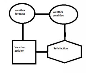
Vacation Influence diagram

You are an outdoors-type and so the choice of activity is affected by the weather. The weather forecast is affected by the weather condition (one hopes!). But you don’t know the actual weather condition, just the forecast (which is why it is a forecast). You choose your activity (box) based on the forecast. The amount of satisfaction you get (lozenge) depends on the activity you chose AND the actual weather condition: observe the two lines leading to the lozenge. There is a standard format:

1. Decision Nodes are presented in rectangles. In the example on the slides, the decision is what activity to pursue when on vacation (climb a mountain? read a book?). Which choice we make mayto some extent be determined by the weather forecast.

2. Uncertainty Nodes are presented in ovals. The weather fore- cast is uncertain and so is the actual weather itself.

3. Outcome Nodes are presented in lozenges. The outcome in the vacation example is how much satisfaction you took from the choice you made for vacation activity. This is a utility.

4. Arcs display the flow of the influence. The actual weather condition affects the weather forecast, which affects your planning. Notice that you are taking a decision on activity in advance ofknowing what the actual weather will be. That is why there is no arc between weather condition and vacation activity.

You can draw influence diagrams quite easily in Excel using the shapes drop-down tool.

There are different outcomes here, which we can be represented as payoffs. The highest payoff comes from matching your choice of activity to the weather forecast and then finding that the forecast matched reality.

13.2 Expected monetary value

the expected monetary value, or EMV, is just the value of some out- come given a particular state of nature, multiplied by the probability of that state of nature. Here, I am using the customary expression ‘state of nature’not necessarily to refer to anything in the natural world, but to a particular set of conditions.

The state of nature has to be mutually exclusive for the probabilities to work. For example, if we have separate probabilities for rain and sunshine, then cannot calculate for rain AND sunshine. The payoffs which resultfrom each state of nature are different, depending on the state of nature.

Let’s motivate this with an example using a friendly farmer as the decision-maker. He has the choice of planting wheat, raising cattle, or some mixture of both. Those three potential decisions represent his range ofchoices. From experience, he knows how much he can expect to receive depending on the weather at the time of harvest. That amount is called the payoff.

He faces three states of nature, representing different weather conditions at harvest. These are rain, clear, and sunny. For each choice and for each state of nature he knows the payoffs which are represented in the cellsbelow.

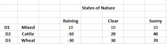
The payoff table for the farmer

There are three decisions and three outcomes, making a total of 9 possible payoffs. Payoffs can be negative, and are not always in terms of money. They could be time, or any other appropriate metric. In the rows we putthe choices available to the decision- maker. In the columns we put the ‘states of nature’ which are the future events not under the control of the decision-maker.

The farmer calculates the probability of each of the three outcomes by working through old weather records. He finds:

probability of raining is 0.4 probability of clear is 0.3 probability of sunny is 0.3 (of course these probabilities must all add up to 1. There could be many more ‘states of nature’ but I have kept them to three for clarity.

The Expected Value is the sum of each probability multiplied by the outcome. In math notation this is:

EMV = ∑ px ∗ x

which in words is: the expected monetary value is the sum of all the outcomes multiplied by their probability. In Excel, use the formula

=sumproduct(array1, array2). This is a mean, or average, with each outcome weighted by its probability. In decisions involving money,

we usually call the Expected Value the Expected Monetary Value (EMV). For the farmer, the EMVs are as below:

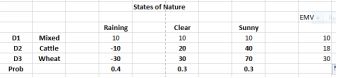
The EMVs for the farmer

I multiplied (horizontally by decision) the payoff by the probability of that payoff and then summed. Usually we choose the decision with the highest EMV, so the farmer should choose wheat. Expected value Youtube¹

Note that a ‘good’ decision is making the best decision at the time with the information to hand at that time. There may be unlucky consequences but provided the analyst has done a thorough job in selecting the optimal outcome at the time, then she should not be blamed!

It will be highly unusual for an outcome of 30 to actually occur. The EMV is just a weighted average and not a prediction.

13.3 Value of perfect information

The farmer might be tempted to ask for advice from a consultant. What is the maximum he or she should pay for the advice? It is the difference between the best case that the farmer calculates and how much he wouldreceive with perfect information. We calculate the value of perfect information by comparing the EMV of the best choice in each state of nature with the EMV without information. If you knew that the weather wouldbe poor, you would select Cattle; clear wheat; sunny wheat again. Then find the EMV with perfect information by multiplying these best options by their probabilities.

The working is: 100.4 + 300.3 + 70*0.3 = 4+9+21 = 34. The best we could come up without perfect information was 30, so the value of perfect information is 34 - 30 = 4. So if someone offered you perfect informationfor a price, the highest that you would pay for the perfect information would be not more than 4.

13.4 Risk-return Ratio

There are other ways of choosing the optimal outcome other than the EMV, although the EMV remains the most commonly used. One common measure is the Return to Risk Ratio, which provides the dollarsreturned per dollar put at risk. For each decision, we divide the Expected Value of the decision by the Standard Deviation of the outcome for that decision. We usually choose the decision with the highest RRR, because then the dollar return for each dollar put at risk is highest. The farmer’s worksheet is below.

Mixed has a zero because the payoffs are all the same. There is no risk. Cattle has the highest at 0.715. This is higher than the RRR for wheat although wheat has the highest EMV. The farmer might want to think moredeeply about the probability of sunny weather at harvest time, because this makes a huge difference.

13.5 Minimax and maximin

A non-probabilistic approach to making choices is the use of maximin and maximax. You can see that your choice depends on whether you are pessimistic (maximin) or optimistic (maximax). If we can somehow obtain probabilities, then a probabilistic approach works best.

13.6 Worked examples

You are planning to market a new coffee-flavored drink. You have a choice between packing the drink in a returnable or non- returnable packaging. Your local government is debating whether non-returnable bottles should be prohibited. The table below shows your profits. If the non-returnable law is passed, you will still get some sales from exports.

Example 1

1. What would be the best decision based on maximin and maximax criteria?

2. A lobbyist tells you that the probability of the government banning non-returnables is 0.7. Assuming the lobbyist is right, what is the best decision based on the EMV?

3. At what level of probability would your decision change?

4. How much would you pay for perfect information?

Answers:

1. Maximin: the worst are 25 and 40. The best is 40, meaning package with returnables. Maximax: the best are 80 and 60. Again returnables.

1. The EMV for returnable is 800.7 + 400.3 = 68. For nonreturn- able it is 250.7 + 600.3 = 35.5. Under EMV, you should use returnable bottles.

2. Set this up as equation, with p the unknown which has to balance both sides 80p + 40(1-p) = 25p + 60(1-p). Solve for

p and get 0.267. So if you hear rumours that suggest the probability is coming down, think again?

3. If we had perfect information, the EVPI is 800.7 + 600.3 = 74. So you should not pay more than 74 - 68 = 6

Example 2

You run a bank. A customer wants to borrow $15,000 for 1 year at 10% interest. You believe that there is a 5% chance that the customer will default on the loan, in which case you will lose all the money. If you don’tlend the money, you will instead place the $15,000 in bonds which return 6% but are risk-free.

1. What are the EMVs of loan and not loan?

2. You have a credit investigation department which can help you with more accuracy in the probability of default. What is the most you should be willing to pay for their advice?

3. Calculate the level of probability of default at which lending the money and investing in bonds have equal EMV.