Business statistics with Excel and Tableau (2015)

What this chapter is about: the previous chapter showed how we could pick the most attractive choice given payoffs and probabil- ities. But it might have struck you that there was little discussion of the risksinvolved and how different people relate to risk. In this chapter we are going to work through picking optimal decisions, taking into account the risk preferences of the decision makers.

Here is a question for you: you are given a lottery ticket which has a 0.5 probability of winning $10,000 and a 0.5 probability of zero. The EMV is therefore 10,0000.5 + 00.5 = $5000. Someone comes along and offers you $3000 for the ticket guaranteed. Would take the sure thing? Or would you hope that you win the $10,000? Most people are ‘risk averse’ and would prefer to give up some of the EMV in exchange forcertainty. The $3000 (or however much it is) is called your Certainty Equivalent (CE) in this particular gamble. The difference between the EMV and the CE is called the Risk Premium. So

RP = EMV - CE

You can think of the certainty equivalent as a selling price. It is usually small when the size of the gamble is small, but increases as the gamble gets larger. Here I am using the term ‘gamble’ because there areprobabilities involved. The certainty equivalent is a useful concept which, amongst other qualities, allows us to categorize approaches to risk.

• Risk-averse. If your CE is less than the EMV of a gamble, then you are risk-averse (and most people are, so nothing to worry about. You’re ‘normal’)

127

• Risk-neutral. Your CE matches the EMV. You play the aver- ages.

• Risk-seeking. You enjoy the gamble inherent in the EMV and need to have a very high CE before you’ll give it up. Most people in business who are risk-seeking usually don’t last very long.Although we sometimes see risk-seeking decisions when your business is in trouble and a huge gamble is the only possible solution

Business decisions are all about risk, and the probabilities them- selves are often unreliable and hard to find. The farmer whose crop- ping decision we studied in Chapter 2 doesn’t know tomorrow’s weather, let alone the weather in six months. We generally prefer to give up some of the EMV in return for more certainty because we are risk averse. That’s why we buy insurance. I know that I will be covered if I smash my car, and Ican even put up with the knowledge that people in Zurich are getting richer because of my aversion to risk.

14.1 Outline of the chapter

Here’s what we’re going to do:

• Describe utility and calculate utilities

• Show how to use the exponential utility function to calculate utilities based on risk tolerance

• Convert those utilities to certainty equivalents which we can rank and compare with the EMVs of the same decision

To rank choices in terms of their certainty equivalent rather than their EMV, we need the concept of utility, which is a numerical measure of how well a good or service satisfies a need or want. Do you prefer to bereading this book, outside eating an ice-cream, or

talking with a friend? You can rank these choices quickly in your head. You can subconsciously allocate utility numbers to the choices and then pick whichever has the highest utility.

Utility numbers help us to rank our preferences, but there are no units and the ranking is individual-specific. In other words, given a set of alternatives, different people may well have different rankings for them. Forthe moment, let’s assume that it is just you whose utilities we are interested in. If we can somehow figure out your utilities for the different outcomes of a business decision, we can use those utilities to help you make a more psychologically satisfying choice.

Utility

The plot below shows a hypothetical utility curve. The utility value is on the vertical y axis and the outcome of a gamble is on the horizontal x axis. Notice two things:

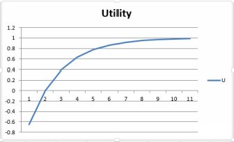
A typical utility curve

*The slope of the line is upwards. This reflects the fact that everyone prefers more money to less

• The rate of increase of the line is decreasing or slowing down. It was steep early on, but towards the end it is almost a plateau. This is because the value of each extra dollar is slightly less thanthat of the previous dollar. This is the marginal utility of money.

14.2 Where do the utility numbers come from?

There are two approaches.

The first involves asking the decision-maker his/her choice between two gambles.

The second uses a utility function, a mathematical function which converts two input variables (risk tolerance and the size of the outcome) into one utility number.

With a utility number in hand we can begin the process of ranking the decisions in terms of utility rather than EMV.

The intuitive model

We’ll work through the intuitive model first and then apply the same thinking to the equation model. Once you get the hang of it, the equation model is quicker and probably more accurate. We’ll use the payoff tablefrom the farmer example, repeated below.

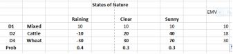
The payoff table for the farmer

We’ll assign a utility number of 1 to the highest payoff and then zero to the lowest. The beginnings of the utility table looks like this:

Payoff Utility

70 1

40

30

20

10

-10

-30 0

Now we need to fill in the gaps. What we’ll do is to use each payoff as a certainty equivalent, and ask this question:

What value of p would make you indifferent between either receiv- ing a guaranteed payoff of the certainty equivalent (in the first case

40) or accepting a gamble of receiving the highest payoff (70) with probability p or losing 30 (the lowest payoff) with probability 1-p. Let’s say that you answer p = 0.9. The expected value of the gamble is 70 * 0.9 + 0.1(-30) = 60.

This is higher than your certainty equivalent of 40, indicating that you are risk averse. The difference between the expected value and the certainty equivalent is the risk premium, and is the amount the individual iswilling to give up to forgo risk.

Continue downwards, certainty equivalent by certainty equivalent and complete the table. I’ve made up the numbers just for illustra- tion. A plot of the utility values is also shown.

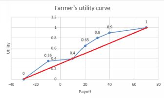
Farmer’s utility curve

If you were risk-neutral, you would prefer to take the gamble and so would be an EMV maximizer. The choice of the risk-neutral person is indicated by the straight line.

Now, let’s replace the payoff values in the farmer table with utilities. We can calculate the expected utilities in the same way as we found the EMVs. The table shows both for comparison. We multiply the utility of eachoutcome with its probability.

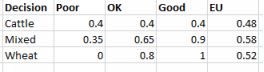
Expected utilities

The famer’s EMV decision would have been wheat (EMV=14) but taking into account his risk preferences, mixed gives the highest expected utility. It makes senses to spread the risk between two completely different crops.

##The exponential utility curve method

It is rather tedious asking so many questions, plus people get tired and confused rather quickly. An attractive alternative is to use a

mathematical function, the exponential utility curve. This requires only one input variable, R, the tolerance for risk. The equation is below:

Ux = 1 − e−x/R

Here x is the payoff; Ux is the utility of the payoff x; and R is the individuals risk tolerance. A person with a large value of R is more likely to take risks than someone with a smaller R value. As the R valueincreases, the behavior approaches that of the EMV maximizer. The plot for someone with a risk tolerance of R = 1000 is below. 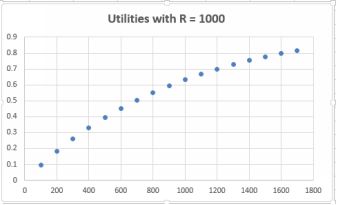Actually performing the calculations to find utility at each level of payoff is easy using Excel, as we’ll see below. But first we have to determine R, theindividual’s tolerance for risk.

Finding risk tolerance

There are two approaches

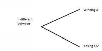
By asking this question: consider a gamble which had equal chances of making a profit of X or a loss of X/2. What is the value of x for which you wouldn’t care whether you had the gamble. In other words, what is thevalue of x for which the certainty equivalent is

zero? The expected value of the alternative is 0.5 x X - 0.5 * (X/2) = 0.25X. As long as X> 0 then the decision-maker is displaying risk- averse behavior, because his/her certainty equivalent is less than the expectedvalue of the gamble. The greater the R, the more tolerant of risk. In his book, Thinking Fast, Thinking Slow, Daniel Kahneman notes that the ‘2’ in the denominator can vary a tad. It isn’t a precise formula, but apparently it comes close: In diagram form:

An al- ternative approach, more used in business and finance, is to employ guideline numbers calculated by Professor Ron Howard¹ , a pioneer of decision-analysis.Based on his years of experience, Howard suggests that the R value for a company is:

• 6.4% of new sales

• 124% of net income

• 15.7% of equity

##Example decision using utility maximisation

What we’ll do here is to examine a decision from both the EMV and Expected Utility angles, using the exponential utility function. The calculation of expected values is the same: the difference is that instead ofmultiplying each monetary payoff by its probability and then adding up, we multiply the utility.

¹https://profiles.stanford.edu/ronald-howard

The decision set-up. All money figures in millions. I run a coffee importing business. I need a special import license to bring in a particular type of coffee. The equity of my company is 12.74. So, my R value is 15.74%of 12.74 = 2.

I have a choice between ‘rush’ and ‘wait’ for the permit.

If I rush, I have to pay a special fee of 5, and there is a 50/50 chance of the permit being granted. If it is granted, I will have sales of 8, giving me a net profit of 8-5 = 3. If it isn’t granted, I still have to pay the 5, but will havesales of only 6, giving me a net profit of 2. First, find the EMV and EU of rushing. The EMV is 0.5x3 + 0.5(2) = 2.5.

Using the exponential curve formula, the utility of 3 is = 1 - exp(- 3/2) = 0.77687. And the utility of 2 is = 1 - exp(-2/2) = 0.632121. The EU for rushing is 0.5(0.77687) + 0.5(0.632121) = 0.704496. All figures are inmillions.

Now for the alternative, which is to wait. In this scenario the probabilities are the same at 50/50, but the cost is only 3 if it is issued, nothing if it isn’t. The sales are the same at 8 and 4. The net profits are 8 - 3 = 5 and 4.The EMV is 0.55 + 0.54 = 4.5. The utilities are U(5) = 1 - exp(-5/2) = 0.918 and U(4) = 1 - exp(-4/2) = 0.865. The EU is 0.50.918 + 0.50.865 = 0.892.

The table below shows the EMVs and EUs.

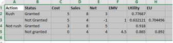
Spreadsheet for the rush decision

But we can go further using certainty equivalents, subject of the next section.

14.3 Converting an expected utility number into a certainty equivalent.

Fortunately there is an easy way to convert expected utilities back to certainty equivalents. It is then straightforward to rank the decisions by certainty equivalents. Remember the concept of the certainty equivalent? The amount of money which it would take for you to sell your gamble? It turns out that we can convert an expected utility number into a certainty equivalent using an equation:

CE = −R ∗ ln(1 − EU )

where ln is the natural logarithm. We use this equation where we are talking profits and want more. In the case of costs, take off the negative sign in front of R.

Above we found EU = 0.704496 for the rush decision branch. That is a CE of

= - 2*LN(1-0.704496) = 2.43814

using Excel’s ln function. For the wait decision, the EU was 0.892, giving a certainty equivalent of = - 2*LN(1-0.892) = 4.451248

Larger CEs are preferred when the outcomes are profits, and smaller CEs when the outcomes are costs. So I’d wait! This confirms the decision made with the Expected Utilities.