Thinking with Data (2014)

Chapter 5. Causality

Causal reasoning is an important and underappreciated part of data science, in part because causal methods are rarely taught in statistics or machine learning courses. Causal arguments are extremely important, because people will interpret claims we make as having a cause-and-effect nature whether we want them to or not. It behooves us to try our best to make our analyses causal. Making such arguments correctly gives far more insight into a problem than simple correlational observations.

Causal reasoning permeates data work, but there are no tools that, on their own, generate defensible causal knowledge. Causation is a perfect example of the necessity of arguments when working with data. Establishing causation stems from making a strong argument. No tool or technique alone is sufficient.

Cause and effect permeates how human think. Causation is powerful. Whenever we think about relationships of variables, we are tempted to think of them causally, even if we know better. All arguments about relationships, even about relationships that we know are only associative and not causal, are positioned in relation to the question of causation.

Noncausal relationships are still useful. Illustration sparks our imaginations, prediction allows us to plan, extrapolation can fill in gaps in our data, and so on. Sometimes the most important thing is just to understand how an event happened or what examples of something look like. In an ideal scenario, however, our knowledge eventually allows us to intervene and improve the world. Whenever possible, we want to know what we should change to make the world be more like how we want it.

We can think about causal arguments in terms of a spectrum, running from arguments that barely hint at causality to arguments that establish undeniable causality. On the near end of the causal spectrum are arguments that are completely observational and not really causal in nature. At most, they vaguely gesture in the direction of causality. They are very useful for building understanding of what a phenomenon is about. Taxonomies, clustering, and illustrative examples stand at this end. Again, these are not causal methods, but they can hint at causal relationships that require further investigation.

The next step in the direction of a full causal explanation is an argument claiming to have found a relationship with predictive power. A predictive relationship allows for planning, but if those variables were different, the outcome might still change as well. Suppose that we understand how likely customers are to quit their subscription to a dating site based on how quickly they reply to messages from other users. We aren’t claiming that getting people to reply more quickly would change the chance that they drop off, only that people who tend to behave like that tend to drop off sooner. Most statistical models are purely predictive.

Moving further along, we have a range of methods and designs that try to eliminate alternative explanations. A design is a method for grouping units of analysis according to certain criteria to try to reduce uncertainty in understanding cause and effect. This is where causal influence actually begins. Techniques like within-subject designs and randomized controlled trials fall here. These methods make an effort to create defensible causal knowledge of a greater or lesser degree, depending on the number of issues stymieing causal analysis that we can eliminate. Randomized controlled trials are at the far end of this part of the causal spectrum.

On the very far end of the causal spectrum are arguments for which a causal relationship is obvious, such as with closed systems (like components in a factory) or well-established physical laws. We feel no compunction in claiming that dropping a vase is the cause of it breaking. Physical examples provide us with our intuition for what cause and effect mean. They are the paragons of the phenomenon of causation, but unfortunately, outside of some particularly intensive engineering or scientific disciplines, they rarely arise in the practical business of data work.

No matter how many caveats we may put into a report about correlation not implying causation, people will interpret arguments causally. Human beings make stories that will help them decide how to act. It is a sensible instinct. People want analysis with causal power. We can ignore their needs and hide behind the difficulty of causal analysis—or we can come to terms with the fact that causal analysis is necessary, and then figure out how to do it properly and when it truly does not apply.

To be able to make causal statements, we need to investigate causal reasoning further. Causal analysis is a deep topic, and much like statistical theory, does not have a single school that can claim to have a monopoly on methodology. Instead, there are multiple canons of thought, each concerned with slightly different scenarios. Statistics as a whole is concerned with generalizing from old to new data; causal analysis is concerned with generalizing from old to new scenarios where we have deliberately altered something.

Generally speaking, because data science as a field is primarily concerned with generalizing knowledge only in highly specific domains (such as for one company, one service, or one type of product), it is able to sidestep many of the issues that snarl causal analysis in more scientific domains. As of today, data scientists do little work building theories intended to capture causal relationships in entirely new scenarios. For those that do, especially if their subject matter concerns human behavior, a more thorough grounding in topics such as construct validity and quasi-experimental design is highly recommended.^[10^]

Defining Causality

Different schools of thought have defined causality differently, but a particularly simple interpretation, suitable to many of the problems that are solvable with data, is the alternate universe perspective. These causes are more properly referred to as “manipulable causes,” because we are concerned with understanding how things might have been if the world been manipulated a bit.

Not all causal explanations are about examining what might have been different under other circumstances. Chemistry gives causal explanations of how a chemical reaction happens. We could alter the setup by changing the chemicals or the environment, but the actual reasoning as to why that reaction will play out is fixed by the laws of physics.

Suppose there is a tree on a busy street. That particular tree may have been trimmed at some point. In causal parlance, it has either been exposed or not exposed to a treatment. The next year it may have fallen down or not. This is known as the outcome. We can imagine two universes, where in one the tree was treated with a trimming and in the other it was not (Table 5-1). Are the outcomes different?

Table 5-1. Consider one tree

We can see that the trimming caused the tree to not fall down, or alternatively, that the lack of trimming prevented the tree from falling down. The trimming was not sufficient by itself (likely some wind or storm was involved as well) and it was not necessary (a crane could also have brought the tree down), but it was nevertheless a cause of the tree falling down.

In practice, we are more likely to see a collection of examples than we are a single one. It is important to remember, though, that a causal relationship is not the same as a statistical one. Consider 20 trees, half of which were trimmed. These are now all in the same universe (see Table 5-2).

Table 5-2. Looking at many trees

It looks at first like we have a clear causal relationship between trimming and falling down. But what if we were to add another variable that mostly explained the difference, as shown in Table 5-3?

Table 5-3. Confounders found

More of the trees that are exposed to the wind were left untrimmed. We say that exposure to the wind confounded our potential measured relationship between trimming and falling down.

The goal of a causal analysis is to find and account for as many confounders as possible, observed and unobserved. In an ideal world, we would know everything we needed to in order to pin down which states always preceded others. That knowledge is never available to us, and so we have to avail ourselves of certain ways of grouping and measuring to do the best we can.

Designs

The purpose of causal analysis, at least for problems that don’t deal with determining scientific laws, is to deal with the problem of confounders. Without the ability to see into different universes, our best bet is to come up with designs to structure how we perform an analysis to try to avoid confounders. Again, a design is a method for grouping units of analysis (like people, trees, pages, and so on) according to certain criteria to try to reduce uncertainty in understanding cause and effect.

A design is a method for grouping units of analysis (like people, trees, pages, and so on) according to certain criteria to try to reduce uncertainty in understanding cause and effect.

Before we stray too far away from multiple universes, one more point is in order. If we had included wind into our investigation of one single tree under different universes, we might see something interesting. After all, there does have to be to be some external agent, like a wind storm, to combine with the trimming or lack thereof to produce a downed tree. This is an illustration of multiple causation, where more than one thing has to be true simultaneously for an outcome to come about.

For data about one tree, reference Table 5-4.

Table 5-4. Multiple causation

Typically, our goal in investigating causation is not so much to understand how one particular instance of causation played out (though that is a common pattern in data-driven storytelling), but to understand how we would expect a treatment to change an outcome in a new scenario. That is, we are interested in how well a causal explanation generalizes to new situations.

Intervention Designs

A number of different design strategies exist for controlling for confounders. In a typical randomized controlled trial, we randomly assign the treatment to the subjects. The justification for the claim that we can infer generalizability is that, because the treatment was chosen randomly for each unit, it should be independent of potential confounders.

There are numerous rebuttals for randomized controlled trials, the details of which would take up many books. The randomization may have been done improperly. The proposed treatment might not be the only difference between groups (hence double-bind experiments). The sample size may not have been large enough to deal with natural levels of variation. Crucially, new subjects may be different in novel ways from those included in the experiment, precluding generalization. If the same people are included in multiple experiments over time, they are no longer necessarily similar to a brand-new person.

In the case of nonrandom intervention, consider observing the stress level of someone for an hour and applying an electrical shock at the 30-minute mark without warning them. It will show a clear evidence of a relationship, but randomization was nowhere to be found. This is an example of awithin-subject interrupted time series design; see Figure 5-1.

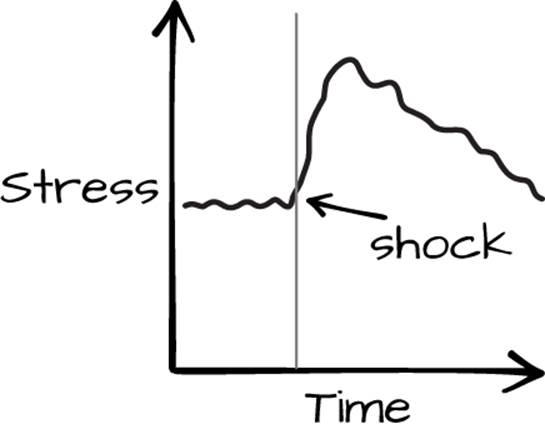
Figure 5-1. A shocking example of within-subject design

The causal relationship between shock and stress is justified on a number of levels. First, if we were carefully observing the subject and didn’t see any other things that would have caused stress, such as a bear entering the laboratory, we have eliminated a large class of potential confounders. Second, we have prior intuition that shocks and stress should be related, so this result seems, prima facie, plausible. Third, the exact timing would be unreasonable to line up with another cause of stress, such as an unpleasant thought that lingered with the subject for the rest of the experiment. Finally, the magnitude of the jump was much larger than variation observed for the same subject prior to the shock.

Were we to perform this same experiment a dozen times, and each time see a similar jump in stress levels, then it would be reasonable to conclude that, for new subjects similar to the ones that we tested on, an unexpected shock would cause a jump in stress levels. That is, we could argue that the relationship is, to some extent, generalizable.

There may still be unmeasured confounders (if all of the experiment subjects were college students, they may have a lower pain threshold than, say, a construction worker) that would stymie generalization. But it is very important to note again that such unmeasured confounders can exist even in a randomized experiment. There may be important, unmeasured aspects of the subjects that can’t be accounted for because all subjects are drawn from the same pool.

A truly randomized experiment would be randomized not only in the treatment, but also in the subjects, and in the pool of potential people or tools that would be carrying out an intervention. That is, we would be picking at random from the potential units (i.e., selecting people from the population at random) and executors of the treatment (i.e., if the treatment is applying a drug, choosing random doctors) in addition to applying the treatment at random. Random subjects and treaters are very rarely applied designs.

Observational Designs

In the case of purely observational designs, we are tasked with employing clever strategies for inferring generalizablity without the ability to intervene.

Observational designs are necessary when it is either impractical, costly, or unethical to perform interventional experiments. Most socially interesting causal estimation problems are of this kind. They frequently occur in business too; it may be advantageous for certainty’s sake to take down a part of a business to see how it affects profit, but the downstream implications are almost always too great to consider doing so. Instead, we have to take advantage of natural differences in exposure or temporary outages to determine the causal effect of critical components.

Natural Experiments

Our best hope in setting up observational designs is to try to find natural experiments. Consider an effort to determine how being convicted of a crime in high school affects earnings from age 25 to 40. It isn’t enough to just compare earning differences between those who were convicted and those who weren’t, because clearly there will be strong confounding variables. A clever strategy would be to compare earnings between those who were arrested but not convicted of a crime, and those who were convicted. Though there are obvious differences in the groups, they are likely to be similar on a number of other variables that serve as a natural control. This is what is known as a natural experiment: we try to argue that we have made a choice about what to compare that accounts for most alternative explanations.

When natural between-subject controls are not available, we can sometimes use methods such as within-subject interrupted time series designs, analogous to the electrical shock example. If sign-ups on a website are rising steadily, and when we introduce a new design for the sign-up page, sign-ups begin to drop immediately, it seems reasonable to assume that the redesign is at fault. But to claim so in good faith (and to make a strong argument), we have to eliminate other contenders. Did the site get slower? Is there a holiday somewhere? Did a competitor get a lot of coverage? By looking at bar charts and maps comparing the sign-ups for different groups of people in different regions, and confirming that the drop is fairly universal, we can strongly justify the redesign as the culprit. We are looking at the same subject and trying to account for alternatives.

The same methodology can also deal with fuzzier problems where we have no natural control group. If we are interested in whether changes in nutrition standards at schools improve test scores, we can go find test score data for many schools where we know that nutrition overhauls were put into place. If test scores (or test score ranking within a given region, to account for changes in the tests themselves) tend to be relatively flat before a nutrition change, then rise, and we have enough examples of this, it starts to be reasonable to implicate the nutrition changes. The justification for the claim of a causal relationship is that there are few reasonable alternative explanations, especially given the proximity in timing, so a causal relationship is the most logical explanation.

What we would have to do to make a good-faith effort is figure out all of the reasonable confounding factors and do our best to account for them. Our conclusion will necessarily be of a less definite kind than if we had somehow been able to randomly give individual kids more nutritious lunches—but such experiments would be not only unethical, but also self-defeating. How would you possibly enforce the restrictions of the experiment without unduly influencing the rest of the environment?

By comparison, just calculating the current test scores of schools that have booted nutrition standards against schools that have not would not be a particularly effective design, because there are likely to be a great number of confounding factors.

This, generally, paints the way for how we do causal reasoning in the absence of the ability to set interactions. We try to gather as much information as possible to find highly similar situations, some of which have experienced a treatment and some of which have not, in order to try to make a statement about the effect of the treatment on the outcome. Sometimes there are confounding factors that we can tease out with better data collection, such as demographic information, detailed behavioral studies, or pre- or post-intervention surveys. These methods can be harder to scale, but when they’re appropriate, they provide us with much stronger tools to reason about the world than we are given otherwise.

Statistical Methods

If all else fails, we can turn to a number of statistical methods for establishing causal relationships. They can be roughly broken down into those based on causal graphs and those based on matching. If there have been enough natural experiments in a large data set, we can use statistical tools to tease out whether changes in some variables appear to be causally connected to others.

The topic of causal graphs is beyond the scope of this book, but the rough idea is that, by assuming a plausible series of relationships that would provide a causal explanation, we can identify what kinds of relationships we should not see. For example, you should never see a correlation between patient age and their treatment group in a randomized clinical trial. Because the assignment was random, group and age should be uncorrelated. In general, given a plausible causal explanation and a favorable pattern of correlations and absences of correlation, we have at least some measure of support for our argument of causality.^[11^]

The other variety of statistical causal estimation is matching. Of matching, there are two kinds: deterministic and probabilistic. In deterministic matching, we try to find similar units across some number of variables. Say we are interested in the effect drinking has on male fertility. We survey 1,000 men on their history and background, and measure their sperm count. Simply checking alcohol consumption history and comparing light and heavy drinkers in their sperm count is not sufficient. There will be other confounding factors like age, smoking history, and diet. If there are a small number of variables and a large number of subjects, we can reduce some confounding by finding pairs of men who match along many or all of the variables, but wherein only one of the two is a heavy drinker. Then we can compare the sperm count of the two men—and hopefully, if we have measured the right controls, it will be as if we had discovered a natural experiment.

If there are a large number of variables (say that diet is determined by a 100-question questionnaire, or we are introducing genetic data), it is more reasonable to use probabilistic matching. The most famous probabilistic matching methodology is propensity score matching. In propensity score matching, we build a model that tries to account for the probability that a subject will have for being treated, also called the propensity. In the alcohol example, we would model the probability of being a heavy drinker given age, smoking history, diet, genetics, and so on. Then, like in the deterministic matching example, we would again pair up similar subjects (this time, those who had roughly the same probability of becoming heavy drinkers) wherein one was a heavy drinker and one was not. We are seeking to create what might be termed an artificial natural experiment.

There are good theoretical reasons to prefer propensity score matching even in the case of a small number of variables, but it can sometimes be worthwhile to skip the added difficulty of fitting the intermediate model.