Make: AVR Programming (2014)
Part III. Advanced AVR Topics
Once you’ve mastered the AVR itself, this last section of the book is dedicated to using modern communications protocols to interface with other devices, building the circuitry you need to drive motors and other electrical devices, and covering a few more of the features of the AVR that you may or may not need every day. The projects here are more involved, and you can read these chapters largely in whatever order you’d like. When you’re done with this chapter, you’ll be ready to tackle almost any project that you can dream up that needs a microcontroller.
Chapter 13 covers a software and firmware technique that makes good use of what you’ve learned about PWM. This enables playback of sampled speech, volume control, and mixing of low-fi digital audio signals. You’ll end up with a clean sine wave, a nice-sounding abstract droney noisebox, and an improved, serial-port playable “piano.”
In Chapter 14 and Chapter 15, I’ll show you some simple (and not-so-simple) circuits that you can use to control almost anything that runs on electricity. DC motors, stepper motors, solenoids, and even household appliances can be put under microcontroller control with some additional circuitry. Although the projects in these chapters are basically just about turning motors, I’m hoping that you’ve got an idea why you’d like motors to turn.
In Chapter 16 and Chapter 17, I cover the two most commonly used modern serial peripheral protocols. This opens up the world of sophisticated digital sensors, high-resolution digital-to-analog converters, and external storage. The demos culminate in integrating a 25LC256 external SPI EEPROM and an LM75 I2C temperature sensor into a long-running temperature logger, but similar techniques let you work with anything that speaks either I2C or SPI.
Chapter 18 and Chapter 19 are all about making the most of the AVR’s scarce memory resources, which enables you to do more cool stuff. Thanks to some clever encoding, you can store 10 seconds of sampled low-fi speech data in the read-only flash program memory, enough to make a talking voltmeter that reads out the current voltage to you using your own voice. And though the chip’s onboard EEPROM isn’t all that fast or abundant, it doesn’t disappear when the power goes out and it’s writable from within your code. I show off by making an AVR secret encoder/decoder that stores the passwords in EEPROM. If you have two with the same key phrases stored in them, you can pass encrypted messages.
Chapter 13. Advanced PWM Tricks
Direct-Digital Synthesis
To create audio that’s more interesting than square waves, we’re going to use PWM to create rapidly changing intermediate voltages that’ll trace out arbitrary waveforms. For now, we’ll content ourselves with a few of the traditional synthesizer-type waveforms (sine, sawtooth, and triangle waves), but this project also lays the groundwork for playing back sampled speech. (When we have enough memory at our disposal, in Chapter 18, we’ll use the same techniques to make a talking voltmeter.) We’ll also be able to change the volume of the sounds and mix multiple sounds together. If you like making spacey, droney sounds or just something more musical than the square wave sounds we’ve been making so far, this is the chapter for you!
Along the way, we’ll really give the PWM hardware a workout. We’ll be running the timer/counter with no prescaling (at 8 MHz) and, frankly, we can use all the speed we can get. Generating fancy waveforms in real-time at 31.25 kHz involves enough math that it’s tough on the CPU as well, and we’ll find that there are just some things we can’t do all that easily. But in my opinion, some of the fun of working with small devices like microcontrollers is seeing how much you can do with how little. I hope you’ll be pleasantly surprised by what is possible.
For starters, we’ll make a simple DDS sine wave generator. Unmodulated sine waves are kinda boring, so the next project demonstrates how to mix different DDS oscillators by taking a few (2, 4, 8, or 16) sawtooth waves and mixing them together. To animate the sound, each waveform is slowly shifted a little bit over in time by different amounts, creating a phasing effect that makes a nice drone sound, and is the basis for a lot of 1990’s basslines when played rhythmically. Finally, the last project adds dynamic volume control, making your nice AVR into a fairly cheesy sounding “piano.” Ah well, beats square waves, right?
WHAT YOU NEED
In this chapter, in addition to the basic kit, you will need:
§ A speaker and capacitor hooked up to the AVR to make sound.
§ (Optionally) a resistor and capacitor pair to make a lowpass filter if you’re going to connect the output to an external amplifier.
§ A USB-Serial cable to play the piano from your desktop’s keyboard.
FREQUENCIES WITHIN FREQUENCIES
As we work through Direct-digital Synthesis, it’s probably a good idea to think of the PWM value you write to OCR0A as being directly translated into a voltage level, because we’ll be varying this voltage level over time to make up the desired audio waveform. So when I say “frequency of the waveform,” I’m referring to how many times the audio voltage-wave cycles per second.
But of course, we know that deep down, the PWM “voltage level” is itself just another, much faster, train of on-off pulses that repeat at the PWM frequency. These pulses are smoothed out so that they appear to be a nearly constant average voltage at the audio-frequency timescale, and you won’t need to worry about them most of the time, as long as your PWM frequency is high enough that your filter does enough smoothing to average them out.
On the other hand, if you’ve switched output from something slow like a speaker to something that responds a lot faster, like a good amplifier or pair of headphones, you may notice some high-frequency noise that you didn’t before. The remedy is to increase the value of the resistor and/or capacitor in your lowpass filter, slowing down its voltage response, so that it damps out the much-higher PWM frequency.
Direct-Digital Synthesis
At the heart of this application is a technique known as direct-digital synthesis (DDS). If you’d like to reproduce, for instance, a sine wave, you start by sampling the voltages along that waveform at regularly spaced intervals in time. Then to play it back, you just output those different voltage levels back over time. You’ll store all of the different sample values (voltage levels) for one complete cycle of your waveform in an array in memory, and then play through this sample lookup table at different speeds to create different pitches.
It’s easy enough to imagine how to play the fundamental note; you would just step through the lookup table at a fixed speed, storing one value at a time in the PWM compare register to generate that voltage. Now to change the pitch, you’ll need to change how quickly you go through the waveform lookup table. The obvious way to do that would be to speed up the playback rate, but there’s no good way to do that with the hardware we’ve got—the system CPU clock runs at a fixed frequency, and to speed up the PWM part, we’d need to also drop down the resolution. There must be a better way.
Instead of changing the clock frequency—how quickly you take each step through the cycle—you change how many steps you take for each clock tick. In order to play a lower note, with a longer wavelength, you play some of the steps for more than a single sample period. To play a higher note, you skip some steps in the waveform table. Either way, the idea is that it takes more or less time to get through one complete trip through the waveform table, resulting in a lower or higher pitch.
There’s still a couple more implementation details left, but for starters, imagine that you went through the lookup table, playing each sample for one PWM cycle each. I’ve written this routine out in pseudocode:
uint8_t waveStep;
while(1){
waveStep++;
OCR0A = lookupTable[waveStep];
// (and wait for next PWM cycle)
}
Now if you want to play a note that was an octave up, you can go through the same lookup table but skip an entry each time, and the output will cycle through the table twice as fast. In the pseudocode example, that would correspond to incrementing waveStep by two each sample (see Figure 13-1). Here, the basic wavetable has 40 samples. Skipping every other step gives you effectively 20 samples to get through the full wavetable. Alternatively, in the same time it took to play one full sample, you’ll get through the wavetable two times by skipping steps. Either way you look at it, the pitch of the output waveform is doubled by skipping steps.
If you wanted to play a note that was an octave down, you’d just need to figure out a way to increment waveStep by 1/2 each time through the loop. This is going to be the secret to DDS. Instead of changing the playback speed of the samples, you change the number of steps you take per PWM cycle.
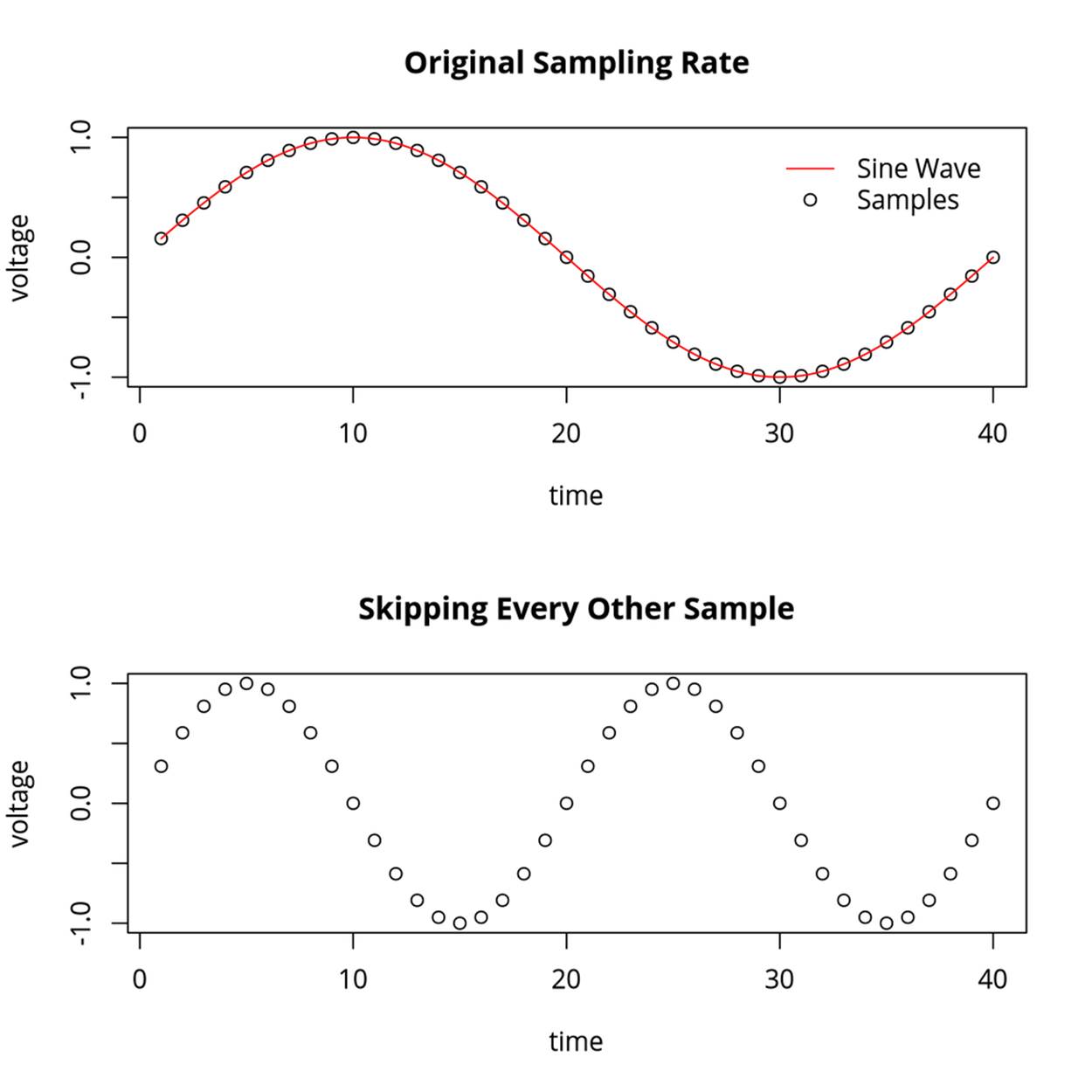
Figure 13-1. Sampled sine wave
Playing a note that’s up an octave was easy—just advance your counter by two—but the math gets complicated when you want to play at a frequency that isn’t an octave. In the 12-tone scale that we’re used to, each key on a keyboard differs in frequency from its neighbors by a factor of the twelfth root of two, or about 1.059463. We can’t multiply waveStep by 1.06 using only integers. We’re going to need to figure out a way to increase our precision.
Getting more precision is actually pretty easy, just use more bits. The secret to getting more precision quickly and efficiently is realizing that it’s easy to convert a 16-bit number into an 8-bit one by bit shifting 8 to the right. So we’ll do our counting in a 16-bit variable, but stick with a 256-step wavetable. Going from the higher precision number to the lower is just a matter of shifting bits to get the waveStep in the lookup table. In the lingo of DDS, we keep track of our position in the wavetable using a 16-bit accumulator, but then we only need to use the most significant eight bits to index the lookup table.
If this seems similar to the trick we used to maintain precision in moving averages in Chapter 12, that’s because it is. There, we kept track of our moving average by multiplying and adding together 10-bit ADC values and then waiting until the last minute to do the division.
Another way of saying exactly the same thing is to imagine that for each of the 256 values in our lookup table, we count to 256 before moving on to the next sample. This lets us control the speed that we play through the waveforms down to 1/256th of what we had before. To play the original base pitch, we now need to add 256 to the accumulator for each sample. Playback at an octave down (taking half a step per sample) is as simple as adding 128 to our accumulator each step. Playing a note that’s a half-step up means changing our accumulator increment to 271 steps. The result is that we’ll advance to the next step most of the time, but sometimes skip one so that the pitch is just a little bit higher. Perfect!
Now our pseudocode looks something like this:
uint16_t accumulator;
uint8_t waveStep;
while(1){
accumulator += 271;
waveStep = accumulator >> 8;
OCR0A = lookupTable[waveStep];
// (and wait for next PWM cycle)
}
SUMMARY: DDS IN A NUTSHELL
You’d like to make a complex analog waveform, and at an arbitrary pitch. How do you do it? The DDS solution is to store a lookup table with the waveform in memory. Every time you need to output a new voltage (in our case using PWM), you advance a certain number of steps through the lookup table and write out the next lookup value to the PWM.
To get more resolution, and thus more tuneability, you keep track of which step in the lookup table you’re on using an accumulator with more precision than the lookup table. Then when you want to look up the corresponding sample, for instance in an 8-bit lookup table, you just use the most significant 8 bits, bit shifting away the least significant bits.
For each PWM cycle, you add a relatively large number to your 16-bit accumulator, then bit shift a copy of the accumulator over by 8 bits to get a step number in the 8-bit range of the lookup table. You look up the corresponding step in the lookup table, and the proper duty-cycle is written out to the PWM.
Making a Sine Wave
So let’s flash in our first DDS example, dds.c. It won’t do anything at first, but if you’ve connected a button and speaker, pressing the button will emit a nice sine wave around 440 Hz. Time to break down the code in Example 13-1.
Example 13-1. dds.c listing
/* Direct-digital synthesis */
// ------- Preamble -------- //
#include <avr/io.h> /* Defines pins, ports, etc */
#include <util/delay.h> /* Functions to waste time */
#include "pinDefines.h"
#include "macros.h"
#include "fullSine.h"
static inline void initTimer0(void) {
TCCR0A |= (1 << COM0A1); /* PWM output on OCR0A */
SPEAKER_DDR |= (1 << SPEAKER); /* enable output on pin */
TCCR0A |= (1 << WGM00); /* Fast PWM mode */
TCCR0A |= (1 << WGM01); /* Fast PWM mode, pt.2 */
TCCR0B |= (1 << CS00); /* Clock with /1 prescaler */
}
int main(void) {
uint16_t accumulator;
uint16_t accumulatorSteps = 880; /* approx 440 Hz */
uint8_t waveStep;
int8_t pwmValue;
// -------- Inits --------- //
initTimer0();
BUTTON_PORT |= (1 << BUTTON); /* pullup on button */
// ------ Event loop ------ //
while (1) {
if (bit_is_clear(BUTTON_PIN, BUTTON)) {
SPEAKER_DDR |= (1 << SPEAKER); /* enable speaker */
accumulator += accumulatorSteps; /* advance accumulator */
waveStep = accumulator >> 8; /* which entry in lookup? */
pwmValue = fullSine[waveStep]; /* lookup voltage */
loop_until_bit_is_set(TIFR0, TOV0); /* wait for PWM cycle */
OCR0A = 128 + pwmValue; /* set new PWM value */
TIFR0 |= (1 << TOV0); /* reset PWM overflow bit */
}
else { /* button not pressed */
SPEAKER_DDR &= ~(1 << SPEAKER); /* disable speaker */
}
} /* End event loop */
return (0); /* This line is never reached */
}
Timer 0 is configured in Fast PWM mode, so for our purposes, think of the value written to the compare register, OCR0A, as representing the average voltage we want to output during that PWM cycle. Note that we’re setting the clock input prescaler to a value of 1, that is to say, no prescaling. For sampled audio, we need all the speed we can get.
In the event loop, we check to see if the button is pressed. When it is, the speaker is enabled for output, and the DDS routine inside the if() statement runs. Just as in our earlier pseudocode example, the accumulator is advanced by a number of steps that determine the pitch, then the 16-bit accumulator is divided by 256 (using bit-shift division) yielding the step of the waveform table that we’re on. Then the lookup takes place, yielding the (signed) integer pwmValue. I keep this variable signed because it’s easier later on when we mix multiple signals together or scale them by volume multipliers, because it’s centered on zero.
SIGNED INTEGERS
Note here that our wavetables are made up of signed integers. Why? It makes volume control and mixing a lot easier. If the waveforms can vary between –128 and 127 and we divide them in half, we’ll get a waveform between –64 and 63, which is still nicely centered, and we can add it together with other waveforms. Only at the last minute, before writing it out to the PWM register, do we convert it to the 0–255 range that we need to fit in the OCR0A register.
Then we load the PWM register, but first we have to wait for the current PWM cycle to finish. This guarantees that we only load up the PWM register with a new value once per cycle, which keeps the sample rate nice and consistent. The OCR is then written to with our signed pwmValue + 128. The number 128 is chosen because the range of signed 8-bit integers goes from –128 to 127, and adding 128 to it maps it nicely into our PWM counter’s 0 to 255 range. Finally, the PWM overflow flag bit is reset by writing a one to it, as described in the datasheet, so that we will be able to detect when we’ve yet again completed a full PWM cycle.
SAMPLE RATE
In this demo, we’re using 8-bit PWM to generate a new average-voltage once per PWM cycle. But exactly how frequently are we playing back each voltage-level sample? We’ll have to do some math.
Because we’re running the AVR off of its internal CPU clock at maximum speed, the CPU clock is 8 MHz. We’re using no prescaling, so the effective PWM clock also ticks eight million times per second. Using an 8-bit PWM, we complete one PWM cycle every 256 clocks, so our resulting PWM frequency is 31,250 Hz.
One of the central theorems of digital signal processing states that you have to sample a sine wave at least twice per period to reproduce it. That is, our current system can reproduce a maximum frequency of 15,625 Hz, which is fairly respectable.
LOWPASS FILTER
If you’re thinking of amplifying the signal from the AVR synth that we’ve just made, you might want to put a lowpass filter between your AVR’s audio out and your amplifier’s audio in. Remember what I said about PWM working to create average voltages when the response of the driven system is slow enough? If you’re running the audio out directly into a speaker, the tiny AVR is not going to be able to push the speaker cone back and forth at anywhere near the PWM frequency, and you’ll be OK.
On the other hand, if you’re plugging the AVR output into an amplifier, the amp may be fast enough to react to the PWM-frequency signals or higher, creating extra noise or even amplifier instability. So let’s cut out the higher-frequency components with a lowpass filter.
The simplest lowpass filter is a resistor in series with the AVR out, followed by a capacitor to ground. See Figure 13-2 for an example. The basis of a lowpass filter is the resistor and capacitor, and their product determines the cutoff frequency of the filter—the frequency above which tones get quieter and quieter. With the values here, all frequencies above 1,600 Hz begin to be attenuated, which assures that our 31.25 kHz PWM frequency is nice and quiet.
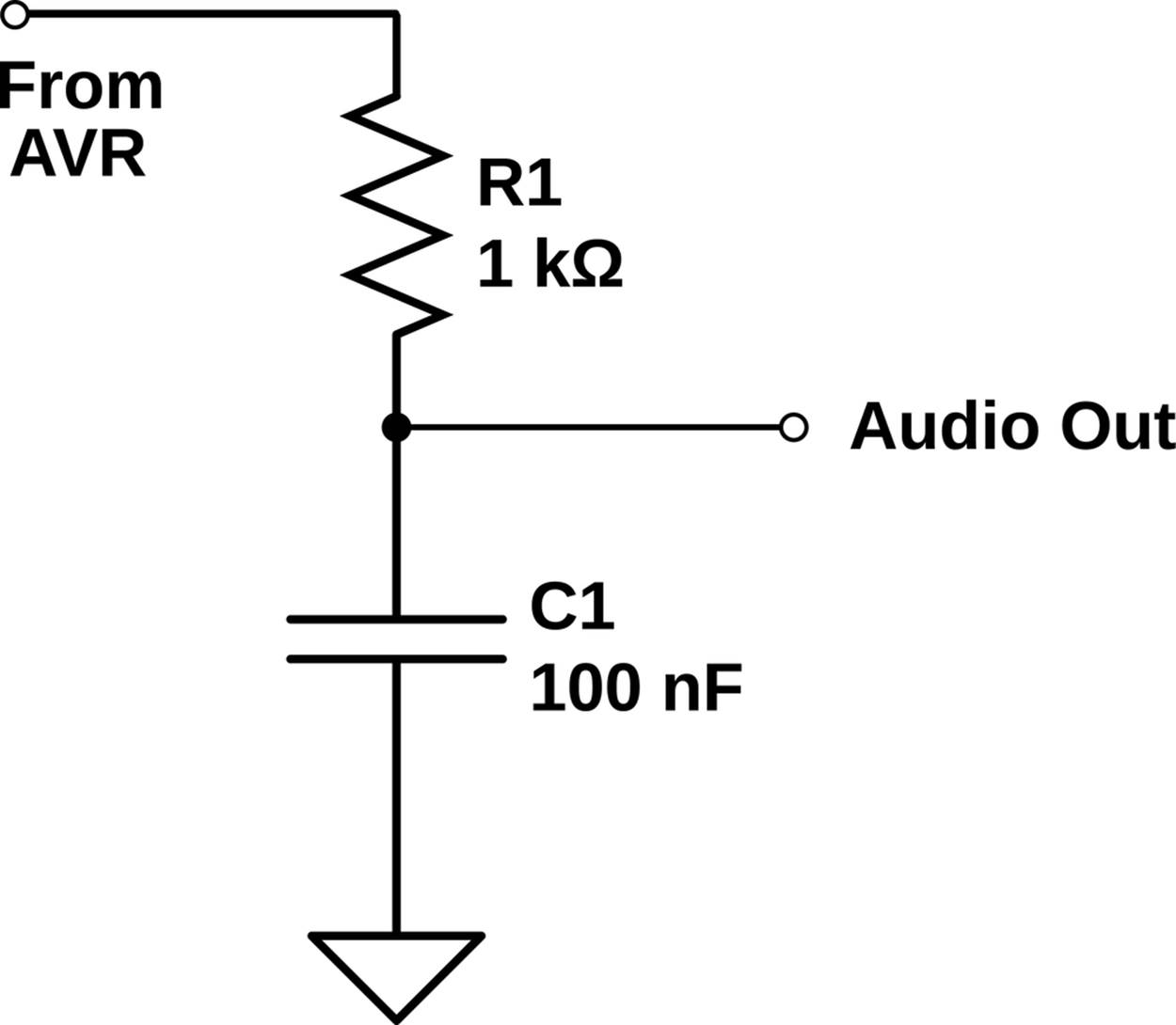
Figure 13-2. Simplest lowpass filter
Next Steps: Mixing and Volume
The nice thing about DDS synthesis is that it’s incredibly easy to mix two or more waveforms together (add the waveform values), or to make sounds louder or quieter (multiply or divide them). Combining different waveforms with dynamic volume envelopes puts us on the road toward real sound synthesis, and being able to mix a few of these sounds together puts real music within reach.
Toward these ends, I’ve included two demonstrations. The first mixes two, four, eight, or sixteen sawtooth waves together and then varies their relative phases. It creates a neat, slowly evolving soundscape, and also introduces us to what happens if our event loop is too slow for our sample update frequency—we end up with a lower pitch. The second example demonstrates a simple way to add a dynamic volume envelope to our sounds. Before when we were playing square waves, the speaker was either on or off. There was no idea of volume. But here, with DDS, if we put out a series of voltages that are 1/2 of the PWM value of another series, the resulting sound will be quieter.
Mixing
First off, load up and flash the fatSaw.c code and give it a listen. The code is a lot like our DDS sine wave code in Example 13-1, but with the waveform lookup table changed, and multiple sound sources playing at once and mixed together. Then start having a look through the code in Example 13-2.
Example 13-2. fatSaw.c listing
/*
Direct-digital synthesis
Phasing saw waves demo
*/
#include "fatSaw.h"
int main(void) {
uint16_t accumulators[NUMBER_OSCILLATORS];
uint8_t waveStep;
int16_t mixer;
uint8_t i;
// -------- Inits --------- //
initTimer0();
SPEAKER_DDR |= (1<<SPEAKER); /* speaker output */
LED_DDR |= (1<<LED0);
// Init all to same phase
for (i = 0; i < NUMBER_OSCILLATORS; i++) {
accumulators[i] = 0;
}
// ------ Event loop ------ //
while (1) {
/* Load in the PWM value when ready */
loop_until_bit_is_set(TIFR0, TOV0); /* wait until overflow bit set */
OCR0A = 128 + mixer; /* signed-integers need shifting up */
TIFR0 |= (1<<TOV0); /* re-set the overflow bit */
/* Update all accumulators, mix together */
mixer = 0;
for (i = 0; i < NUMBER_OSCILLATORS; i++) {
accumulators[i] += BASEPITCH;
waveStep = accumulators[i] >> 8;
// Add extra phase increment.
// Makes shifting overtones when
// different frequency components add, subtract
if (waveStep == 0) { /* roughly once per cycle */
accumulators[i] += PHASE_RATE * i; /* add extra phase */
}
mixer += fullSaw15[waveStep];
}
mixer = mixer >> OSCILLATOR_SHIFT;
/* Dividing by bitshift is very fast. */
} /* End event loop */
return (0); /* This line is never reached */
}
The first thing you’ll notice is that I’ve moved the standard preamble, with include files and defines, off to its own fatSaw.h file. Many people like to do this to reduce clutter in the main loop. I’m doing it here mainly to save space. In the fatSaw.h file are some definitions relating to the number of voices we’d like to produce and even the same initTimer0() function that we used in our first DDS program. (C programmers will argue that putting significant code in an .h file is bad practice, because other people aren’t expecting it there. I agree, but in the same sense that macro functions are tolerated in .h files, I beg your indulgence with a couple bit-twiddling initialization routines.)
Just inside the main() routine, notice that we’re defining an array of accumulators because we have to keep track of not just one note’s location in the wavetable, but up to 16. Moving on to the event loop, the first chunk should look familiar. The routine waits for the current PWM counter loop to complete, then loads the OCR and resets the overflow flag bit.
The mixer chunk is where the interesting action lies. Notice that we’ve defined a 16-bit signed integer called mixer, in which we’ll add up all of the waveform values from the individual digital oscillators. So for each oscillator, we advance its accumulator (here, all by the same amount) and then use a bit shift divide to find out which step in the waveform table we’re on. At the end of the mixer code loop, we look up our value from the table and add it to the mixer.
The fun stuff lies in the middle. Here, we advance the accumulator by a few steps in the accumulator’s phase each time around the cycle. Each oscillator gets moved forward in its accumulator by a different amount, however, which results in the different versions of the exact same note slipping against each other in time, sometimes peaking all at the same time (when the note sounds lowest) and other times offset from each other (producing overtones). The effect is a slowly changing drone which I find a little hypnotic if it’s just left running.
Finally, after we’ve looped through all of the oscillators and added their values together, the mixer is rescaled to be in the 8-bit range again. But remember that it’s a signed 8-bit integer, so we’ll have to convert it to an unsigned integer again and add 128 to go from the range –128..127 to 0..255. Here again we use a bit-shift divide. You can try the code out with a regular division, and you’ll be able to hear the difference—the pitch will shift down because the AVR isn’t able to make its sample updates every 32 microseconds.
DEBUGGING FOR SPEED
There are limits to how much math you can do per cycle at this sampling rate. If you run the PWM as fast as you can, at 31,250 Hz, then there are less than 256 available CPU clock cycles per sample update. This is plenty of time to do some complex operations on a single voice, or simple operations on a few voices, but if you try the fatSawdemo with eight or sixteen voices, you’ll end up missing the 31.25 kHz update frequency. The result is that you miss PWM updates and the effective sampling frequency drops to 15,625 Hz and a lower pitch results.
There are two good ways to diagnose these types of high-speed issues in code—look at the generated assembly code or set a pin to toggle at different points in the code, enabling you to look at the timing of individual sections on an oscilloscope.
The avr-gcc suite that we’re using includes a reverse-assembler (avr-objdump) that will turn your compiled code into quasi-readable assembly code. With your makefile you can type make disasm and then have a look at the resulting fatSaw.lst list file. Though working through AVR assembly is beyond the scope of this book, you can get a rough idea of timings by seeing where your C code translates into long blocks of assembly.
The other useful high-speed debugging method is to blink LEDs and read them on an oscilloscope. For instance, if you’re interested in how long the fatSaw routine waits for the PWM overflow flag to clear, you could turn an LED on just before the loop_until_bit_is_set(TIFR0, TOV0); and turn it off right after. The time spent looping here is equal to the free time you have for code in the event loop, and the period of the waveform will be the 256 cycles * 1/8 microsecond = 32 microseconds that you’ve got to update the PWM register. If the waveform looks jittery or takes longer than 32 microseconds, it’s a warning sign that you’re not making your desired sample rate.
So if you really want to do something elaborate with a whole lot of virtual oscillators, you’re going to need more processing power. If a factor of two or three in speed will let you do what you’d like, you can clock the AVR’s CPU up to 20 MHz by syncing it to an external crystal or oscillator. If you really need much more than that, as one often does for high-quality audio synthesis, the AVR may not be able to keep up, and you may need a dedicated digital signal processing (DSP) chip or to offload the sound generation to a real computer and save the AVR for controlling the interaction and interfacing. But before we give up on the good old AVR, let’s see if we can’t make some interesting musical sounds.
Dynamic Volume Control
Our next step toward getting something that sounds more natural is to put a volume envelope on the sound. When you hit a piano key, a string gets hit by a hammer and goes rather quickly from being still and quiet to vibrating and making sound. This phase is called the attack. Then the string settles into its main vibratory modes, with the settling speeds referred to as the decay rate and sustain level. Then when you let go of the key, the sound dampens out fairly quickly at a speed called the release rate. If you wanted to model a piano sound, you’d need to get at least these volume dynamics right. Let’s see what we can do.
ADSR ENVELOPES
This attack-decay-sustain-release volume envelope that we’ll be using for our “piano” is pretty much the standard across all sorts of real synthesizers from the 1970s to the present.
Load up the code adsr.c and let’s get started. If you’ve never played around with an old synthesizer that has an ADSR volume envelope before, you may want to tweak the defined envelope values in adsr.h for a while. Try a long attack, maybe 220, to see how that smooths out the initial sound by more slowly ramping in the initial volume. Try setting the sustain level higher or lower and the sustain time and release rates to play with the default note length.
Once you’re done with that, let’s dive into the code in Example 13-3.
Example 13-3. adsr.c listing
/*
Direct-digital synthesis
ADSR Dynamic Volume Envelope Demo
*/
// ------- Preamble -------- //
#include "adsr.h" /* Defines, includes, and init functions */
int main(void) {
// -------- Inits --------- //
uint16_t accumulator = 0;
uint8_t volume = 0;
uint16_t noteClock = 0;
uint16_t tuningWord = C1;
uint8_t waveStep;
int16_t mixer;
uint8_t i;
char serialInput;
initTimer0();
initUSART();
printString(" Serial Synth\r\n");
printString("Notes: asdfghjkl;'\r\n");
SPEAKER_DDR |= (1<<SPEAKER); /* speaker output */
// ------ Event loop ------ //
while (1) {
// Set PWM output
loop_until_bit_is_set(TIFR0, TOV0); /* wait for timer0 overflow */
OCR0A = 128 + (uint8_t) mixer;
TIFR0 |= (1<<TOV0); /* reset the overflow bit */
// Update the DDS
accumulator += tuningWord;
waveStep = accumulator >> 8;
mixer = fullTriangle[waveStep] * volume;
mixer = mixer >> 5;
/* Input processed here: check USART */
if (bit_is_set(UCSR0A, RXC0)) {
serialInput = UDR0; /* read in from USART */
tuningWord = lookupPitch(serialInput);
noteClock = 1;
}
/* Dynamic Volume stuff here */
if (noteClock) { /* if noteClock already running */
noteClock++;
if (noteClock < ATTACK_TIME) { /* attack */
/* wait until time to increase next step */
if (noteClock > ATTACK_RATE * volume) {
if (volume < 31) {
volume++;
}
}
}
else if (noteClock < DECAY_TIME) { /* decay */
if ((noteClock - ATTACK_TIME) >
(FULL_VOLUME - volume) * DECAY_RATE) {
if (volume > SUSTAIN_LEVEL) {
volume--;
}
}
}
else if (noteClock > RELEASE_TIME) { /* release */
if ((noteClock - RELEASE_TIME) >
(SUSTAIN_LEVEL - volume) * RELEASE_RATE) {
if (volume > 0) {
volume--;
}
else {
noteClock = 0;
}
}
}
}
} /* End event loop */
return (0); /* This line is never reached */
}
Because this code is a little bit complex, let’s start with an overview. The first chunk of code is just the usual DDS routine, waiting for the PWM timer to overflow to set the next value. Then a variable tuningWord gets added to the accumulator, which will result in the desired pitch. Finally, the 16-bit mixer stores the wavetable value scaled up by volume and down by the maximum volume (as a bit-shift division).
Polling USART
Next, the code polls the USART for new data, and sets the tuningWord depending on which key has been pressed. It also sets a noteClock variable, which is incremented to keep track of time for the volume envelope. Finally, a lot of code space (relatively speaking) is spent changing the volume of the note as it evolves over time and the noteClock advances.
The section where we check up on the USART is not particularly difficult to understand, but because it’s such a useful technique, I’ll expand on it a little bit. In contrast to the last few times we’ve used the serial port where we wait in an infinite loop for serial data to arrive, in this example, we implement a nonblocking, polled USART input. “Polled” in this sense means that we check to see if new data has come in once every time we go around the event loop. If yes, we process it. If not, we just keep on looping.
Polling for serial data works because the USART raises a “receive complete” (RXC0) flag in the status register (UCSR0A) when it gets a new byte of data in. This flag is automatically cleared whenever the USART data register (UDR0) is read, so we don’t have to tell the USART that we’re ready for the next byte; it knows automatically.
And because the event loop is running really frequently in this example, at 31.25 kHz, the delay between a received character and playing the note is so short that a human will never know. On the other hand, when you really need instant response to incoming serial data, you can always feel free to use an interrupt! You have lots of options.
ADSR Envelope
The other section of the code that still needs explanation is the dynamic ADSR volume envelope calculation bit. An idealized (continuous-volume) version of an ADSR envelope is shown in Figure 13-3. In our implementation, because we can’t tell how long the key was pressed, we set a sustain time instead of waiting until the key is released. Otherwise, it’s standard.
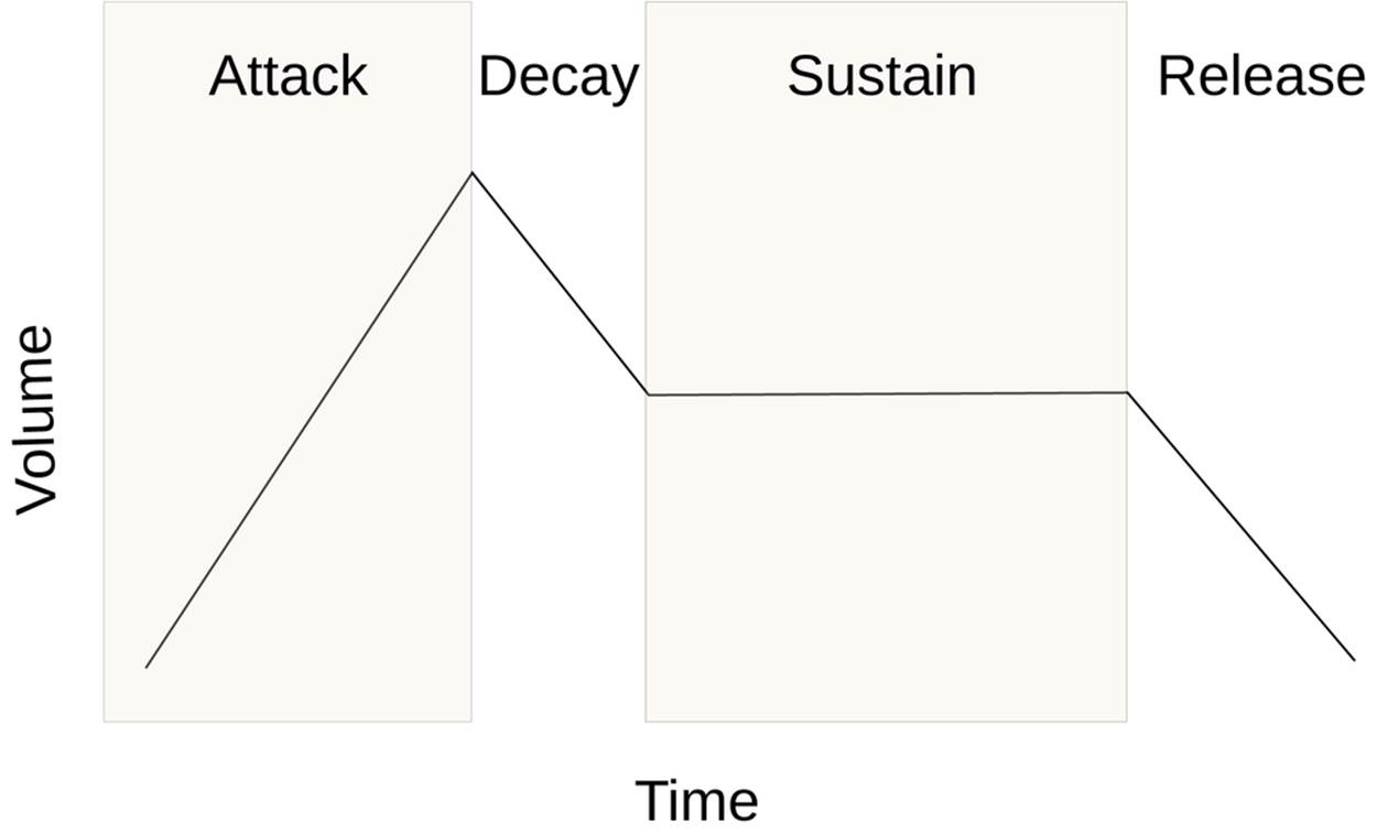
Figure 13-3. ADSR volume envelope
The code first determines which phase of the ADSR it’s in: attack, decay, sustain, or release. If it’s in the attack phase, it increases the volume by one level per ATTACK_RATE ticks of the noteClock. As an example of how this works, consider the clock and volume starting off at zero and an ATTACK_RATE of three. Initially, the clock and volume*ATTACK_RATE are all zero, so no action is required. When the clock ticks over to one, the clock part is larger, and the volume is incremented. Now volume*ATTACK_RATE is equal to three, and the volume won’t be incremented again until clock tick three, and so forth.
The other stages of the ADSR work the same, only instead of starting from having the clock at zero, the decay phase starts at the end of the attack phase so the ATTACK_TIME is subtracted off the clock. Because the volume remains constant during the sustain, we just ignore it, and pick back up when it’s time to start decreasing the volume again during the release phase.
Auxiliary Files
This program relies on a lot of other files to function, and though they’re kinda cool from a musical synthesis perspective, they’re out of the scope of this book.
The waveform tables are loaded up from header files that store our lookup table in RAM as a 256-byte array. The routines that generate these waveforms are in a Python program that’s attached, generateWavetables.py. You can also make your own to correspond to whatever timbre you’d like the DDS sounds to take on. However, RAM memory is limited to 1 kB on the ATmega168 chips, and burning a quarter of that memory up for each waveform you’d like to play is dangerous. You’ll be fine loading two waveforms into memory, but three is dangerous and loading four will certainly end up with different sections of memory overwriting each other and impossible to debug glitches. You’ve been warned.
ARRAYS IN MEMORY
The way that we’re storing the waveform tables in memory isn’t particularly efficient—we’re storing them in the chip’s scarce dynamic memory (of which the chip has only 1 kB) even though the values don’t change. A much better approach is to store the waveforms in the flash program memory space, where we’ve got 16 kB of space, and we know for sure that some of it is sitting empty. I’ll cover the use of program memory in Chapter 18, so if you need to build a synthesizer with a whole bunch more wavetables, feel free to skip ahead.
Or you can use your head—I’m not exploiting any of the symmetry in the sine waves. Because the second half of the cycle is just the same as the first half but with a negative sign, you could easily cut memory storage in half. You could also cut the storage in half again if you observe that for each sample in the first quarter, the same sample in the second quarter is just 255 minus the first.
I thought the DDS code was complicated enough without this extra optimization, so I left it as simple as possible. This means you can’t really use more than three waveforms in the same program without running into trouble.
The scales that are loaded up in scale.h are generated by the Python file generateScale.py. These accumulator increment values are dependent on the processor speed we choose as well as on using 8-bit PWM. If you’re interested in other pitches, or nontraditional pitches, feel free to play around with the scales.
Anyway, DDS synthesis is a great tool. If you’re content with a lower bit-depth or a slower sample rate, creating music this way is entirely within the power of an AVR chip, even for multiple voices simultaneously. Indeed, you’ll see in Chapter 18 that it’s fairly easy to make reasonable-sounding human sampled speech, for instance. And although we’re aiming at audio here, bear in mind that similar techniques can be used (with proper buffering for current-handling capability) to smoothly accelerate and decelerate motors, or any other situation where you need time-varying voltage waveforms.
All materials on the site are licensed Creative Commons Attribution-Sharealike 3.0 Unported CC BY-SA 3.0 & GNU Free Documentation License (GFDL)
If you are the copyright holder of any material contained on our site and intend to remove it, please contact our site administrator for approval.
© 2016-2026 All site design rights belong to S.Y.A.