Make: AVR Programming (2014)

Part II. Intermediate AVR

Chapter 12. Analog-to-Digital Conversion II

Accurate Voltage Meter and the Footstep Detector

In Chapter 7, you learned the basics of using the ADC to convert continuous analog voltages into digital numbers that you can use in your AVR code. In this chapter, I’ll go over some of the extra details that you’ll need to work with many real-world devices.

In particular, you’ll find that not everything works on the same 0 V to 5 V range that your AVR’s ADC wants to use, so we’ll have to talk a little bit about input voltage scaling. You may also find that sometimes you want a little bit more accuracy than the AVR’s 10-bit ADC can deliver. When this is the case, you can either buy a separate ADC chip or use a software technique known as oversampling to get a couple more bits of effective resolution. We’ll combine these two ideas to make a surprisingly accurate voltmeter that can read from 0 V to 15 V in hundredths of a volt.

We’ll also build up a project that I use in my own home to detect footsteps and turn on a light for the stairs. It detects footsteps using a sensor that’s tremendously versatile for detecting sound and vibration—the piezo-electric disk. Because the piezo (for short) creates an AC voltage, we’ll look into biasing it so that the voltage always lies in the middle of the range that the AVR likes to see—a technique you’ll also want to use for microphones, for instance.

The software tricks in making a very sensitive footstep detector involve ADC data smoothing. In any real-world circuit, there’s always some background noise, and the true value that we’d really like to measure often lies buried somewhere within it. When making a very sensitive device, like our piezo vibration sensor, figuring out the difference between this background noise and our desired signal is very important. In this project, we know that the “volume” from the vibrations of a footstep is a fairly short signal, while the background noise is basically constant. We’ll use a moving average to get a good idea of the sensor’s natural bias point as well as the average magnitude of the background noise. Then, when we see a sensor reading that’s outside this range, we’ll know that it’s a footstep.

WHAT YOU NEED

In this chapter, in addition to the basic kit, you will need:

§ A battery whose charge you’d like to measure.

§ A USB-Serial adapter for voltage display.

§ Three resistors of the same value for an input voltage divider.

§ A standalone voltmeter to calibrate the AVR voltmeter.

§ A piezo disk, preferably with wires attached, for the footstep sensor.

§ Two 1M ohm resistors to provide bias voltage for the piezo.

So without further ado, let’s get down to it. It’s time to learn some pre- and post-ADC signal conditioning.

Voltage Meter

The story of this voltmeter project is that I was building a battery charger that knew when to stop charging a 9 V rechargeable battery. When charging nickel-based rechargeable batteries, the voltage across the battery increases until the battery is full, at which point it levels off and even drops just a little bit. To use this slight voltage drop as a clue that the battery was 100% charged, I needed to read out a voltage into the AVR that was outside of the 0–5 V range and needed enough resolution that I could detect the tiny little dip in charging voltage and not overcharge the battery.

So the design specs are to make a voltmeter that measures a voltage in the range 0–15 V with resolution down to two decimal places—10 mV. “Wait just a minute!” I hear you saying, “The ADC only measures 10-bits or 1,024 steps, which are just about 15 mV each over a 15 V range. How are you going to get more resolution than that? And how are you measuring up to 15 V with just a 5 V power supply?”

Measuring higher voltages is actually easy enough. We simply predivide the voltage down to our 5 V range using a voltage divider. To measure up to 15 V, we only need to divide the input voltage down by a factor of three, which we can do fairly accurately with just three similar resistors. That’s the easy part.

To get extra resolution in the measurement, we’ll use oversampling, which is a tremendously useful technique to have in your repertoire. The idea behind oversampling is that we take repeated measurements from our ADC and combine them. This almost sounds like averaging, but it’s not the same. When we average four numbers, for instance, we add up the four numbers together and divide by four. When we oversample 4x, on the other hand, we add the four numbers together and divide by two, increasing the number of bits in our result by one. To bump up our 10-bit ADC to 12-bit precision, we will use 16x oversampling, adding together 16 samples, dividing by four, and keeping the extra factor of four (two bits) to get us up to 12 bits.

We’ll also use an AVR-specific ADC trick to reduce measurement noise. Because the CPU generates electrical noise while it’s running, Atmel has provided functionality that shuts down the CPU and lets the ADC run on its own. Using this special “ADC Noise Reduction” sleep mode turns off the CPU and I/O clocks temporarily but leaves the ADC clock running while the ADC conversion takes place, and then wakes the chip back up once the ADC-complete interrupt fires. This reduces noise on the power supply due to either the CPU or any of the other pins switching state, which helps measurement accuracy.

By combining ADC Noise Reduction sleep mode and 16x oversampling, we can actually get just a little more than two decimal places of accuracy in our measurements, but not quite enough to justify reporting the third decimal place. Getting much more precision than that requires a very stable and accurate power supply for the AVR, and a good voltmeter to calibrate it against, so let’s call 10 mV good enough and get to it.

OVERSAMPLING

Oversampling seems like magic. You take a 10-bit sensor, add up 16 observations, and then divide down by four and declare that the result is good to 12 bits. What’s going on?

When you take a normal average of a few samples, it has the effect of reducing the variability of the measurement. Intuitively, if one ADC reading happens to be a bit high, the next one might just be a bit low. There are some statistics that I’m sweeping under the carpet (a central limit theorem), but the end result is that the variability of an average drops as the square root of the number of measurements in the average increases. Qualitatively, taking averages of measurements tends to smooth out noise, so if you’ve got a measurement that’s jumping all over the place due to sensor noise, you can take bigger and bigger averages until it’s smooth enough for you. When we took moving averages before, we were doing just that.

Adding numbers together (and not averaging) results in a larger number of bits in the sum. If you add two 10-bit numbers, the result can be as large as an 11-bit number. Add up four 10-bit numbers, and the result requires 12 bits. But the last bit isn’t any less noisy than the samples that went into the sum. You’ve got a bigger number for sure, but not a more precise one.

When oversampling, you take many samples to get more bits and then take a (partial) average to smooth the result out so that it’s precise enough to justify the extra bits. In our example, we add up 16 samples, enough to end up with a 14-bit number, and then we divide by four (equivalently, drop the least-significant two bits). Now we’ve got 12 bits that we’re pretty sure of.

Anyway, this has all been hand-waving around some fairly serious mathematics. I hope that it gives you a little bit of faith in oversampling—it’s a great technique that you should know. To use oversampling, all you have to know is that if you want n more bits of resolution, you take a sum of samples and bit shift the result n times to the right (dividing by 2n).

The main limitation is that you have to take these samples before the true input value changes by more than one least significant bit, so oversampling is mainly a technique for slowly varying signals relative to the sampling speed. You can almost always use oversampling for anything that happens on a human time scale, but it’s going to slow you down too much for audio. There’s a three-way trade-off between speed, precision, and cost. 16x oversampling is 16 times slower than sampling directly, but two-bits more precise and free. If you need faster and more precise, you can always pay money for a better ADC!

For more on oversampling and the AVR’s ADC converter, see the Atmel application note “AVR121: Enhancing ADC resolution by oversampling.”

The Circuit

Electrically, there’s really not much going on here. We want to be able to measure voltages up in excess of AVCC, so we divide the input down with a voltage divider. The voltage divider has twice as much resistance between the battery and the AVR pin as between the AVR and ground, so it’s a divide-by-three voltage divider. Using three identical resistors, the circuit will look like Figure 12-1 on a breadboard.

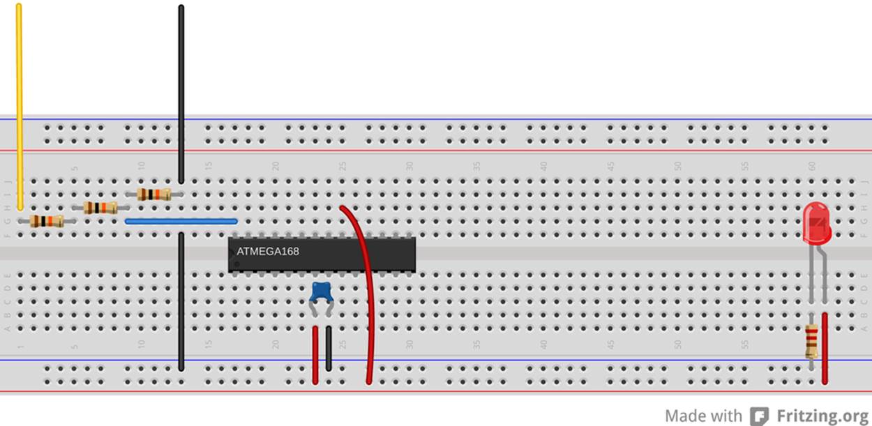
Figure 12-1. 3x voltage divider

For our voltage divider, we want this to be as close to a true 3x division as possible, which means having twice as much resistance in the “top” half of the voltage divider as in the “bottom.” Unfortunately, the standard resistor value series jumps from 10k to 22k ohms, so there’s no good 2x ratio available without special ordering. Long story short, the easiest thing to do is buy yourself three resistors and make your voltage divider with them, using two in series for the “top” resistor to drop 2/3 of the voltage.

RESISTOR TOLERANCE

In the real world, 10k ohm resistors don’t really measure exactly 10k ohm, but are rather specified with a tolerance. Common tolerance grades are 1%, 5%, and 10%. One of the cruel realities of economics is that 1% tolerance resistors cost more than 5% resistors, which cost more than 10% resistors, and this means that you’ll almost never find a 10% tolerance resistor that’s closer to the nominal value than 5%—the manufacturer could sell it as a 5% tolerance resistor for more money.

On the other hand, due to improved manufacturing techniques, 1% resistors are pretty cheap these days, almost to the point that it’s not worth it to check. So if you’re lucky, you might find that a 5% resistor is accidentally within 1% of the target value, but I wouldn’t count on it. Ten years ago, you’d almost never find one.

Voltage scaling in general

Here, were using a voltage divider to predivide down a 0–15 V range to fit the AVR’s 5 V maximum. This is a special case of a more general problem: the sensor’s range doesn’t always match up with the voltage range that works well for the microcontroller.

If your sensor outputs between two and three volts, and you’re measuring with an ADC that reads between zero and five volts, you’re wasting a lot of the ADC’s precision. Using a five-volt ADC reference voltage, and ten bits resolution, we get 5/1024 volts per step, or just under 5 mV per step. Between two and three volts, there are only around 200 of these steps, so in that situation, you’ve only got around one-fifth of the possible resolution—the sensor will never output high or low enough to make use of 80% of the ADC’s range. The point is that you make best use of the ADC’s resolution when the voltage range of the ADC matches the voltage range of the sensor.

Basically, we want to rescale and recenter the sensor’s signal to match the voltage-measurement range of the AVR. Rather than rescaling the sensor’s output, it’s often easier to change the ADC’s voltage reference. There are two easy things we can do to match the sensor’s output voltage range with the ADC’s measurement range, and make best use of the 10 bits that we’ve got.

The AVR chips give us choices in voltage reference, which is extremely handy, often meaning that we don’t have to use any frontend prescaling circuitry. In our examples, we’re using VCC as our voltage reference, which is the simplest solution if your sensors are able to output in that range. If you can easily design your voltage-divider type sensors so that they’re between VCC and GND, and use most of the available voltage range, you’re done.

Another possibility when the range of the sensor is less than VCC, but the lowest signal is still at ground, is to use a voltage divider on the AREF pin (with a capacitor to stabilize it). This can work very well, with the caveats that cheap resistors are often only accurate to 10% or so, and the values can change with temperature, leaving you with higher or lower absolute voltage measurements depending on the weather. On the other hand, two matched 1% quality resistors in a voltage divider can give you a 2.5 V reference that’s just about as accurate as your VCC value—if the resistors have the same resistance, the effects of changing temperature will cancel out.

The AVR chips also have an internal voltage reference, which is nominally 1.1 V, but can range from 1.0 V to 1.2 V across chips. This isn’t as bad as it sounds—the voltage level for your particular chip will stay nearly constant over time, temperature, and VCCfluctuations, which is especially handy if you’re running a circuit on batteries. If your sensor’s output range is between ground and something less than 1 V, the internal reference voltage is the way to go. If the input signal range is higher than 1 V, but you’re worried about a changing VCC affecting your measurements, it’s often worth it to divide down your input signal and use the internal voltage reference. This is a good trick to use with battery-powered circuits, where VCC changes as the battery drains.

With all these options for the ADC’s reference voltage, the hard part of matching the sensor to the AVR is making sure that the minimum voltage stays above ground.

For many sensors, like microphones and the piezo transducer that we use here, the voltage swing is naturally symmetric around ground, guaranteeing that we’ll lose half of the signal unless we recenter it to capture the otherwise negative half of the signal. The good news is that with these sources, we don’t need the DC level from the sensor. We only care about changes in voltage, say from our voice reaching the microphone or ground tremors reaching our seismograph. In those cases, the simplest circuit to implement is to use a capacitor to block the DC voltage and a voltage-divider circuit to bias the center voltage. We’ll use this approach in The Footstep Detector.

When you have a sensor with an extreme range, or if you require biasing, and if the DC level matters, then things are more complicated. With an operational amplifier (op-amp) it’s fairly straightforward to build a signal conditioning circuit that’ll get your sensor signal just where you want it in terms of bias voltage and range, but that’s adding a level of complexity to the circuit that’s beyond this book.

The Code

Because we want the voltmeter to be accurate and we’re using AVCC as the voltage reference, we’re going to have to very accurately measure the AVCC to get the scaling right. This means at least two or three decimal places, which means using a decent voltmeter.And we’ve got the divide-by-not-exactly-three voltage divider in the circuit, which we’ll also have to measure and calculate around. While I usually avoid doing much floating-point math—math with noninteger numbers—on the AVR, I’ll make an exception here because the code is simpler that way. The trade-off is that the floating-point math libraries take up more program space and are much slower to execute than integer math, but for this example, none of the timing is critical, and we have memory to spare. Let’s start looking into the code in Example 12-1.

Example 12-1. voltmeter.c listing

/* ADC Voltmeter

* Continuously outputs voltage over the serial line.

*/

// ------- Preamble -------- //

#include <avr/io.h>

#include <util/delay.h>

#include <avr/interrupt.h>

#include <avr/sleep.h> /* for ADC sleep mode */

#include <math.h> /* for round() and floor() */

#include "pinDefines.h"

#include "USART.h"

/* Note: This voltmeter is only as accurate as your reference voltage.

* If you want four digits of accuracy, need to measure your AVCC well.

* Measure either AVCC of the voltage on AREF and enter it here.

*/

#define REF_VCC 5.053

/* measured division by voltage divider */

#define VOLTAGE_DIV_FACTOR 3.114

// -------- Functions --------- //

void initADC(void) {

ADMUX |= (0b00001111 & PC5); /* set mux to ADC5 */

ADMUX |= (1 << REFS0); /* reference voltage on AVCC */

ADCSRA |= (1 << ADPS1) | (1 << ADPS2); /* ADC clock prescaler /64 */

ADCSRA |= (1 << ADEN); /* enable ADC */

}

void setupADCSleepmode(void) {

set_sleep_mode(SLEEP_MODE_ADC); /* defined in avr/sleep.h */

ADCSRA |= (1 << ADIE); /* enable ADC interrupt */

sei(); /* enable global interrupts */

}

EMPTY_INTERRUPT(ADC_vect);

uint16_t oversample16x(void) {

uint16_t oversampledValue = 0;

uint8_t i;

for (i = 0; i < 16; i++) {

sleep_mode(); /* chip to sleep, takes ADC sample */

oversampledValue += ADC; /* add them up 16x */

}

return (oversampledValue >> 2); /* divide back down by four */

}

void printFloat(float number) {

number = round(number * 100) / 100; /* round off to 2 decimal places */

transmitByte('0' + number / 10); /* tens place */

transmitByte('0' + number - 10 * floor(number / 10)); /* ones */

transmitByte('.');

transmitByte('0' + (number * 10) - floor(number) * 10); /* tenths */

/* hundredths place */

transmitByte('0' + (number * 100) - floor(number * 10) * 10);

printString("\r\n");

}

int main(void) {

float voltage;

// -------- Inits --------- //

initUSART();

printString("\r\nDigital Voltmeter\r\n\r\n");

initADC();

setupADCSleepmode();

// ------ Event loop ------ //

while (1) {

voltage = oversample16x() * VOLTAGE_DIV_FACTOR * REF_VCC / 4096;

printFloat(voltage);

/* alternatively, just print it out:

* printWord(voltage*100);

* but then you have to remember the decimal place

*/

_delay_ms(500);

} /* End event loop */

return (0); /* This line is never reached */

}

The event loop is straightforward; sample the voltage by calling the oversample16x() function, scale it up, and then print it out over the serial port. But in order to run the ADC while the chip is sleeping and incorporate these values in with the oversampling routine, a few things need to be taken care of.

Sleep mode

Making use of the ADC sleep mode is not too hard, once you know how. First, notice that we included avr/sleep.h up at the top. This isn’t strictly necessary—it defines a few macros that save us from having to look up which bits to set in the datasheet. But then again, as long as it’s there, why not use it?

Next, turn to the initialization function setupADCSleepmode(). The first line, set_sleep_mode(SLEEP_MODE_ADC);, actually just runs SMCR |= (1<<SM0); under the hood, but isn’t it easier to read with the defines? Whichever way you spell it, a bit is set in the hardware sleep mode register. That bit tells the AVR to enter ADC sleep mode (halt CPU and I/O clocks and start an ADC conversion). When the ADC-complete interrupt fires off, the chip wakes back up and the ISR is called and handled.

Wait a minute—what ISR? We don’t really need an ISR because we’re sampling on command from a function and sleeping until the ADC is done. But because we’ve enabled the ADC-complete interrupt to wake up out of sleep mode, the code has to go somewhere. The next line, EMPTY_INTERRUPT(ADC_vect);, is specific to the GCC compiler and tells it to set up a fake interrupt that just returns to wherever it was in the code. EMPTY_INTERRUPT() basically exists just for this purpose—creating a quick, fake ISR that we can trigger when we need to wake the processor up from sleep modes.

SLEEP MODES

The AVRs have a bunch of different sleep modes that put some of the internal clocks to sleep until some interrupt condition wakes the chip back up. The basic idea is that you can save power by shutting down the hardware that you’re not using at any given time, and waking the chip up when an interrupt or timer comes in that it needs to handle.

For instance, you’ve already seen how you can set up a timer as a system tick that takes care of handling time for you instead of using _delay_ms() routines. If you don’t have much else to do with the CPU at the time, you might as well let the CPU doze off a bit to save power. Using the idle mode, the lightest sleep mode, is perfect in this case. In idle mode, the CPU clock is shut down, and any interrupt will wake the chip back up. The timer clock, ADC clock, and I/O clocks will all keep running in the background, so you can use idle mode instead of a wait loop and the CPU will wake up with each timer overflow that calls an ISR (like our system ticks). You can even use idle mode if you’re transmitting or expecting serial I/O, as long as you’re handling your serial input from an interrupt service routine and remember to enable the interrupt.

ADC noise reduction mode is the mode we’re using here. It not only shuts down the CPU and I/O clocks, but it also triggers an ADC conversion after the CPU has stopped, and wakes everything back up once the ADC is done, which is exactly what you’d want. How cool is that? (But note that if you’re expecting I/O during the ADC sampling time, you’ll miss it.)

Power down mode is the other sleep mode that I use a lot. It’s the most aggressive of them all—shutting down all of the internally generated clocks and peripherals. From a power-usage perspective, you’re basically turning the chip off. The AVR will still wake up if it receives any external interrupt like a button being pressed, which is handy if you’d like to implement an on/off button. If you’re not using the reset pin for anything else, it makes a nice power-on button to wake the chip back up from power down mode.

You can read up on all of the other sleep modes in the datasheet under the section called “Power Management and Sleep Modes,” where it has a very nice table showing you which peripherals get turned off in which modes and what interrupts will wake the chip back up.

Oversampling

All of the work in oversampling is done in the function oversample16x(). There’s not much to say here, because it’s such a straightforward application. One gotcha is that there is a practical limit on how much we can oversample, set by the size of the variable that we collect up the sum of the samples in. Here, I used uint16_t oversampledValue to keep track of our 16 10-bit samples, and that works out fine. In fact, it’s big enough to contain the sum of 64 10-bit values, so if we needed to oversample even more, we could.

The other thing to note while we’re here is that we could change the bit-shift division in the last line of oversample16x() to divide by 16, and the result would be a regular average of 16 values. This is useful when we’d like to smooth out noise in the sample, and the result will be a 10-bit number that’s more stable than any individual ADC reading by itself.

So to sum up the meat of this project, we can get extra resolution by oversampling, and we can reduce noise to the ADC by using the ADC-specific sleep mode to shut down the CPU while sampling. And we can handle higher-than-5 V voltages by simply using a voltage divider before the ADC. Putting all this together with a stable 5 V voltage reference and some careful calibration, we can easily get 12 bits of data from the 10-bit ADC—enough to detect a 10 mV drop on a charging battery.

The Footstep Detector

In this project, we’ll be using the ADC and a sensor to make essentially a DIY accelerometer, but one that’s specifically tuned to detect very small vibrations like taps on a tabletop, tiny earthquakes, or in my case, a person walking up the stairs. I’ll show you a couple of ways to make the system more or less responsive. I love this project.

The sensor that we’ll use to do this can be found for a few bucks or less, and can be scavenged from a whole ton of cheap commercial products: things like musical greeting cards and tiny buzzers. The piezoelectric disk, or piezo for short, is a crystal that deforms (slightly) when you apply a voltage to it, or conversely develops an electric voltage when you deform it. The first direction, voltage to deformation, gives you a tinny-sounding speaker, super-precise control over laser deflection mirrors, or inkjet printer heads. The reverse direction, deformation to voltage, lets you build force sensors, high-end acoustic guitar pickups, electronic drum pads, and the vibration-sensor in this chapter, not to mention barbecue grill lighters, where the piezo voltage is high enough to make a spark.

PIEZOS

Piezoelectricity was discovered in 1880 by Jacques and Pierre Curie. Yes, that Pierre Curie, who also discovered that magnets lose their pull when they are heated to the Curie temperature, and whose discoveries with his wife about radioactivity got them the Nobel Prize, thanks in no small part to a sensitive piezoelectric electrometer. If you asked me to choose between which discovery was more influential, I’d be hard-pressed to answer. The crystal that’s providing the high-frequency timebase for nearly every computer and radio device you own? Piezoelectric. Pierre Curie should have gotten two Nobel Prizes.

Almost all piezoelectric substances are crystals or ceramics that have a lattice-like molecular layout, and all the molecules arrange themselves in a somewhat rigid three-dimensional grid. The molecules in the crystal are also polar—they have a positively charged and negatively charged end. When you compress a piezoelectric crystal, these molecules realign and the voltage across the crystal changes. When you let go, the molecules swing back to their original orientation. This makes expansion and contraction of the crystal result in a voltage change, and vice versa.

The kind of piezo disk that we’ll be using is actually a thin layer of piezoelectric crystal that’s glued to a metal disk on one side and has a conductive layer on the other. The metal disk keeps the fragile crystal from breaking, and the voltage between the conductive layer and the disk varies with compression or bending. Because the crystal is an insulator this two-plate arrangement is basically a capacitor, and the electrical symbol looks like one, but with a box representing the crystal between the plates. But, as I said before, a piezo is special type of capacitor, one that also generates a voltage when bent or squeezed.

What this means for us is that we can put a constant, DC voltage across the piezo and the piezo will charge up to that voltage and just sit there. Then when we bend or compress the piezo, we’ll get a temporary positive or negative AC voltage superimposed on the DC voltage. In the project here, we’ll read this AC voltage into the AVR to detect vibrations.

Piezo voltages can be quite large (tens of thousands of volts for the piezos in barbecue igniters) if you really smack the piezo. Because the source of the voltage change is the realignment of molecules in a crystal, a form of static electricity, the total amount of current flowing in or out of the piezo is reasonably small, so you’re not going to hurt yourself. Still, we protect the AVR’s static-sensitive inputs against possible voltage spikes with the resistor on the input to the AVR’s pin PC2 in this section’s circuit, and you should probably avoid hitting the disk with a hammer or a drumstick once it’s hooked up. We’re trying to detect footsteps here.

The Circuit

The first thing you’re going to need to do is get your hands on a piezo disk, ideally one that comes with wires already soldered to the disk and conductor. The easiest way to do this is to scrounge one out of a cheap device that was using the piezo to make noise—it’ll come already wired up! If you don’t have a supply of junked electronic noisemakers handy, most electronics stores will be able to sell you a piezo buzzer for just a few dollars that’ll come encased in a black plastic enclosure that serves to make it louder. A few piezo discs are shown in Figure 12-2. Your mission, should you choose to accept it, is to liberate the piezo disk inside by smashing the black plastic without destroying the disk.

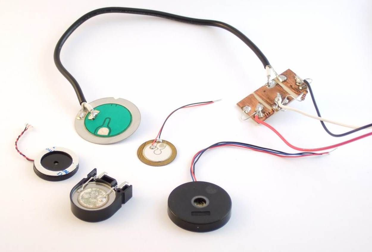
Figure 12-2. Piezo discs in the wild

As mentioned in Piezos, piezo sensors will make positive or negative voltages depending on whether it’s bent one way or the other. The AVR’s ADC, however, only reads from 0 V to VCC, with no range for negative voltages. The workaround is to bias the piezo toVCC/2, and to do this we’ll use a voltage divider. That way, a small negative voltage on the piezo will add together with the VCC/2 bias voltage to produce an overall voltage just under VCC/2 at the AVR’s input pin.

In Figure 12-2, you’ll notice that the green piezo element is connected to a piece of circuit board that has the voltage divider biasing circuit already soldered on. This simplifies breadboard connections later on. All you have to do is hook up the red wire to VCC, the black wire to GND, and then the white wire provides the biased sensor value, ready to hook straight into the ADC.

Figure 12-3 demonstrates how this is done. Using high-value resistors for R1 and R2 is important here because you don’t want the bias voltage to swamp out small changes in the piezo voltage. Because the voltage divider is always pulling the voltage back to theVCC/2 center point, the smaller the resistance in the voltage divider, the stronger the pull back to center will be because more current is flowing through the divider. For our setup you can easily substitute 10 megohm resistors if you’d like more sensitivity, or drop down to 100k ohm resistors if it’s too sensitive. On the other hand, if you make the biasing voltage resistors too large (like 100 megohm resistors or no biasing at all), the biasing at VCC/2 may not work at all, and the voltage will wander away from the fixed bias point.

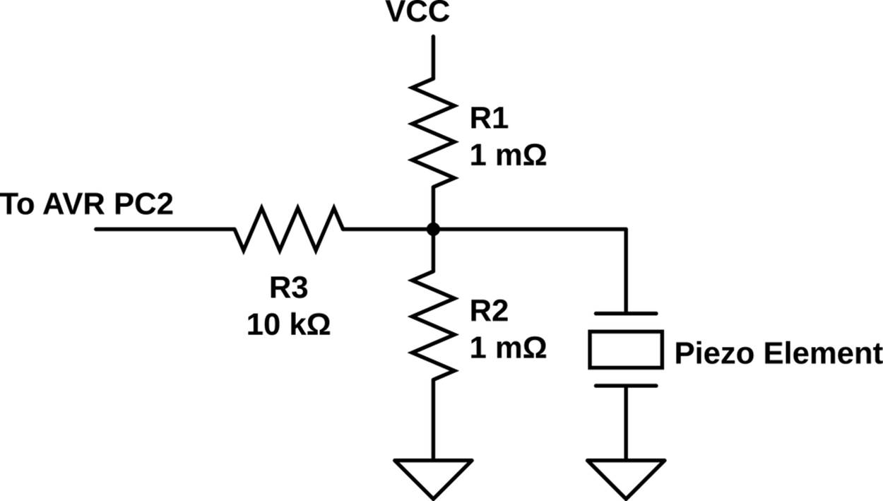
Figure 12-3. Piezo biasing circuit

It’s worth noting that this circuit actually represents a generally applicable solution to a common problem: any time you have an input signal that can be both positive and negative with respect to the AVR’s ground, you’ll want to provide a pair of bias resistors to pull the “ground” of the sensor up to the middle of the AVR’s voltage range so that you can measure both the positive and negative sides of the signal. For instance, if you were connecting a microphone to the AVR, you’d also use a voltage-divider biasing circuit just like this connected to the AVR’s input. Additionally, you’d need to add a capacitor between the sensor and the bias circuit/AVR pin in order to keep the microphone from changing the DC level away from this mid-voltage bias point. Here, the piezo’s own capacitance serves the same purpose, making adding another capacitor pointless. You should end up with something that looks like Figure 12-4 on your breadboard.

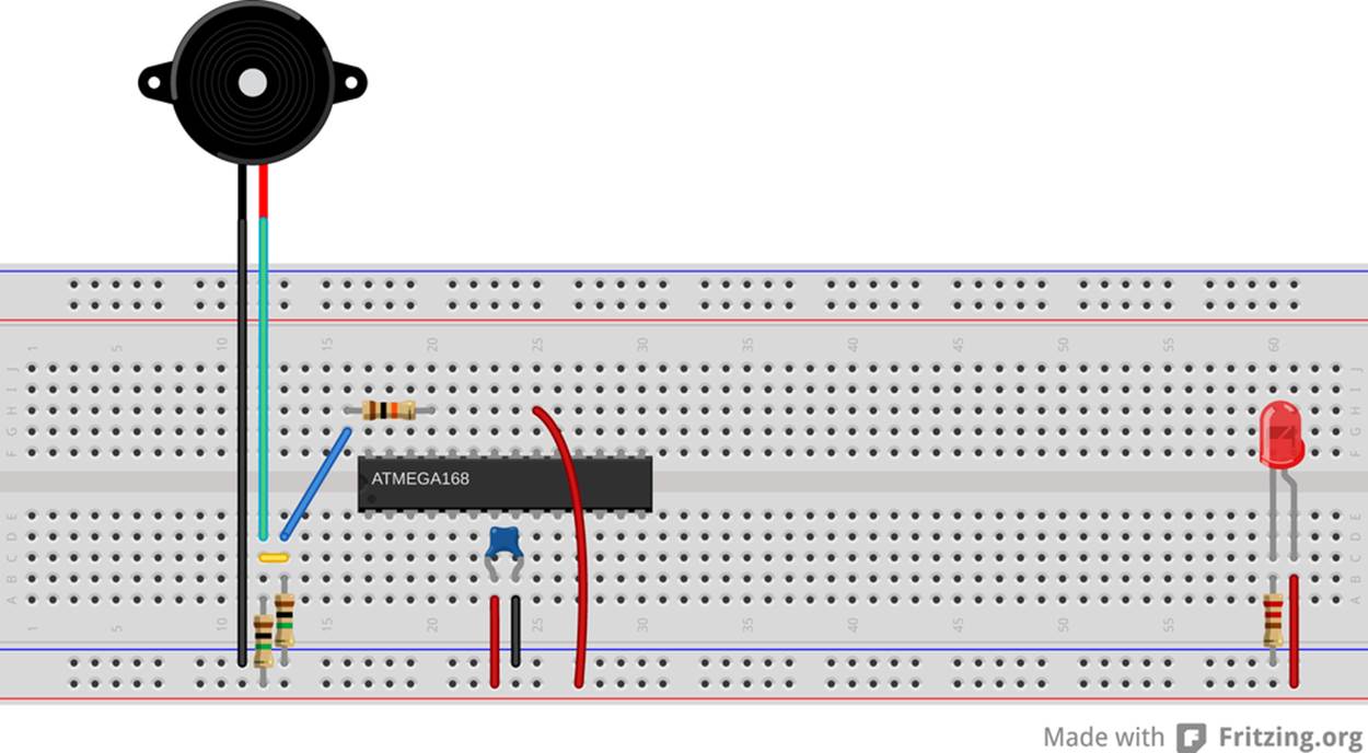
Figure 12-4. Piezo footstepDetector breadboard

Finally, the input resistor R3 in Figure 12-3 protects the AVR from the case that we generate a too-high or too-low voltage by really whacking the piezo sensor. The input resistor works like this: inside the AVR, the pins have diodes that prevent too high or low voltages from frying the circuitry, but these diodes can only handle a limited amount of current before the AVR gets burnt out. The input resistor gives us a little bit more assurance that if the external voltage goes too high or too low, not much current will flow. You can increase sensitivity by leaving this resistor out, but you’d better be careful not to hit the piezo sensor hard.

So that’s the electronic circuit: three resistors and a piezo disk. The rest of the sensor design is mechanical engineering. For a table-based seismometer with maximum sensitivity, you’ll want to do what they do inside commercial accelerometers—put a weight on the end of a beam to magnify the effect of the force and wedge the piezo and the beam together in something solid.

For the beam, anything from a ruler to a piece of scrap two-by-four will do. Tape some coins or something moderately heavy to the far end of the beam, and clamp the near end of the beam to your table, wedging the piezo sensor between the table and beam so that any force applied to the table relative to the weight is magnified by the leverage. (You may need to take precautions against your beam shorting out the conductor and disk sides of the piezo. A piece of electrical tape should work.) With this setup I can detect someone walking up the stairs that lead to my office while the piezo is sitting on my office desk.

I’ve also gotten pretty good performance just by resting something heavy on the piezo. At the moment, I have the piezo sitting on my desk with a pint glass holding it down as shown in Figure 12-5. As the table is vibrated up and down, the inertia of the pint glass provides the squeezing force that creates a voltage in the piezo. This setup is much simpler and can still detect my footsteps anywhere within the room. It’s blinking along with each keystroke even as I type this.

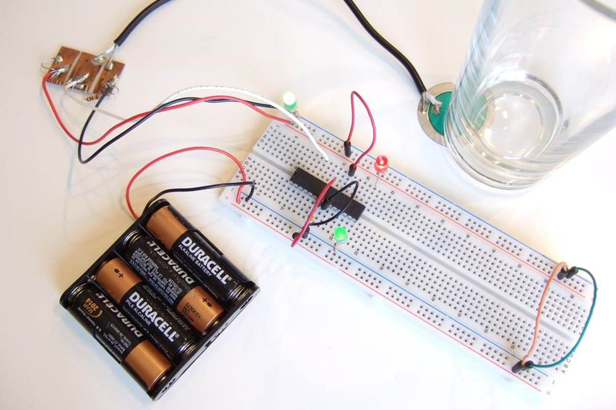
Figure 12-5. Piezo footstep detector setup

Once you’ve got the piezo set up with either a weight or a weight on a beam, you can reduce the sensitivity of the detector in firmware. How loud a signal on the piezo must be in order to count as a footstep is stored in a variable called paddind. You can optionally hook up a potentiometer to pin PC5, which is also ADC channel 5 to control this parameter directly. We’ll read the voltage off the pot, bit shift the value to scale it, and use the result to create a dead band in the center of the ADC’s range where the software doesn’t react. This is useful if you’d like the accelerometer to detect a hard tap on your desk, but not react to each and every keystroke as you type.

And as long as we’re at it, it’s nice to have some LEDs for feedback. If you haven’t pulled the LEDs off of the PB0-PB7 bank, you’ve got nothing more to hook up. If you have, attach LEDs to PB0, PB1, and PB7. Your breadboard should now look like Figure 12-6.

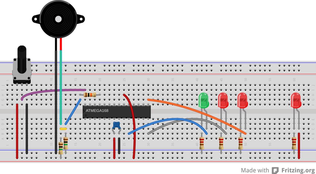
Figure 12-6. Piezo breadboard with optional potentiometer

The Theory

My real-life application for the piezo vibration detector is actually a footstep-activated light for the stairs in my house. The AVR continually reads the ADC and the piezo, and when it finds a vibration that is large enough, it turns on a LED light strip that lights up the stairs. In the final version, I actually combine an LDR circuit with the vibration sensor here so that it doesn’t turn on the lights in the daytime, but let’s focus on the vibration sensing part. We’ll discuss how to turn on and off light strips (and motors and other electrically large loads) in Chapter 14.

My device turns the light strip on for a few seconds when vibration due to a footstep on the stairs is detected, and goes off automatically after the stairs are still again. In the code, I implement the timeout by restarting a countdown timer every time vibration is sensed.

Because I don’t know how hard my footsteps will be, or how much background vibration there is in the house, or how much background electrical noise the sensor sees, I want the sensor to be somewhat auto-calibrating. And because the sensor’s rest voltage is determined by a two-resistor voltage divider, I don’t want to have to recalibrate the firmware between one version of the device and another in order to account for the variation among resistors. So let’s see how we can handle all of these issues in our firmware.

First off, let’s tackle the problem of finding the bias voltage of the piezo. While ideal bias resistors provide a midpoint voltage of 2.5000 V, you may have slightly different real-world values for two nominally 1 megohm resistors, and end up with a bias voltage of 2.47 V or so. Deviations from a perfect VCC/2 biasing voltage will manifest as both the minimum and maximum observed ADC values being higher or lower than 511—the midpoint in the ADC’s 10-bit range. To make the sensor maximally sensitive, that is, to measure the smallest differences between the ADC value and its midpoint, we need to get this midpoint value measured accurately.

Unfortunately, any time we try to measure the bias voltage, it will have some electrical or physical background noise added on top of it. That is, if we make two ADC readings, they’ll probably have different results. On the other hand, the additional noise voltage will be high sometimes and low other times, and if we take an average, the noise will sum up to zero. The strategy is then to take a good long-run average and use that as a measure of the bias value. In order to make the AVR sensor maximally sensitive, it’s important to get this average spot on, and this’ll give me a chance to show you some important details for implementing exponentially weighted moving averages (EWMA) with integer math. (Hold on to your hats!)

Even with a perfect measure of the central value, there is still a limit to how sensitive we can make the footstep detector. We want to pick a value on either side of the central value and and say that when the ADC reads outside these values, a footstep has been detected. If it weren’t for noise in the system, we could pick values just on either side of the middle, bias value. In the real world, we’ve got some range of (possibly even large) ADC values that we shouldn’t treat as footsteps, because they’re just the background noise.

The next moving average trick is to track the noise volume so that we can pick our footstep-detection thresholds outside of it. We do this by taking an average of just the positive values (those greater than the midpoint) and a separate average of just the negative values. When there is no external signal present, the difference between these two averages should give a good idea of the average noise volume. This will increase the sensitivity when this noise is relatively quiet, and we can hope to hear fainter footsteps, and to decrease the sensitivity if there’s a lot of background noise to avoid “detecting” footsteps when none were present.

Exponentially Weighted Moving Averages

This section is going to go into a little bit of math. It’s just a little algebra, but if you’re more into programming the dang AVR than thinking about what it all means, feel free to skip on down to the The Code. On the other hand, exponentially weighted moving averages (EWMA) are a tremendously flexible and simple-to-use tool once you get used to them, so it’s probably worth a bit of your time here understanding what’s going on.

Imagine that we have a sensor reading every second. We’ll call the raw values where the t labels which second the reading is from. A time series of our data is the whole list of etc. That is, it’s the whole measured history of our sensor value. We’ll call our average series . Every time we get in a new sensor value (), we’ll update our average value (), so it ends up being another time series.

A regular moving average of our x’s just takes, for instance, the last five readings and averages them together. If there’s some noise in the readings, it’ll hopefully be high in a few of the five readings and low in the others, so that the average value is close to the “true” underlying sensor reading that we’re looking for. Every second that we get a new sensor reading, we drop the oldest entry out of the average and add in the new one. That’s the “moving” average part—the values that are being averaged together move along with our growing dataset so that we only take an average of, say, five values at a time.

The more terms you choose to average together in your moving average, the better you’ll average out the noise signal. If you average 10 values together, for instance, you’ll have a better chance at seeing both high and low noise values. On the other hand, you’ll be including sensor information from 10 seconds ago into your average value this period. There is always this trade-off between smoothing the values out better and having the average be up to date.

For the AVR to calculate a five-value moving average, we’ll need to store five previous values from our sensor. To store 10, we’ll need to dedicate even more RAM to the averaging. It’s usually not a big deal, but it is possible to use up a lot of memory if you’re tracking a few variables with very long moving windows.

My preferred average, the EWMA, only needs two values to work: the current sensor reading and the current average value. Instead of averaging a bunch of values together, in the EWMA, we only need to average two values: the current value and the average value from the last observation. The only complication here is that we don’t take an equal average between the two, but a weighted average where we put more weight on the past value (usually) than on the present. For instance, in this chapter’s code, we’ll average 1/16th of the current value with 15/16ths of the average from last period.

And finally, because what we’re after is an accurate value for the bias voltage, we’ll want to take some care making sure we calculate everything right. This means avoiding doing division whenever we can, and taking extra care to get the rounding right when we dohave to divide. Even if we make sure to always divide by a power of two, so that we can use a bit shift, we still lose some information every time we divide. As an example, 7/2 = 3.5, but if we’re only using integers, we round up to 4. But 8/2 is also 4, so if we’ve only got the divided-by-two version, we can’t be sure whether it came from a seven or an eight.

Anyway, to the EWMA. In what follows, I’m going to be assuming an EWMA with a 1/16, 15/16 split between the new value and the average. It should be obvious how to generalize this to any other fraction:

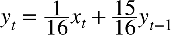
That is, we calculate this period’s EWMA by taking a weighted average of one part this period’s sensor value and many parts of the previous EWMA value.

The secret to keeping the EWMA accurate is to put off the dividing-by-m part until we absolutely have to. Multiply both sides by m and we have:

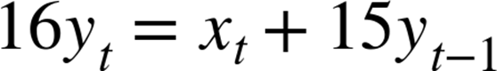
and we’re almost there. Now we have m times the EWMA on the left side, and no dividing at all. But when we come to next period, we’ll need on the right side instead of the that we have. Easy enough, we could subtract off one if we knew it. Because we’ve got , we can subtract off .

But, as I mentioned earlier, when C divides, it just throws away the remainder. There’s a trick to making C “round” for us, and it involves adding or subtracting half of the denominator into the numerator before dividing.

ROUNDING AND INTEGER DIVISION

C does integer division differently than you or I would. If you were dividing two numbers and wanted an integer result, you’d first figure out what the decimal value was (with integer value and remainder) and then round up or down accordingly. C, on the other hand, figures out the integer part and throws away the remainder. For example, 16/8 = 2, 17/8 = 2, and even 23/8 = 2. (24/8, at least, is 3).

It turns out that we can fool C into rounding by preadding half of the denominator before we divide. In our example of dividing by eight, we need to add four to the number up front before the division: (16 + 4) / 8 = 2, (19 + 4) / 8 = 2, but (20 + 4) / 8 = 3, etc. If you want your integer divisions to be “rounded” to the nearest integer, remember to add or subtract this correction factor of half of the denominator before dividing.

The final equation, minimizing the effects of division and adding in a rounding factor looks like Equation 12-1.

Equation 12-1. Optimized EWMA equation

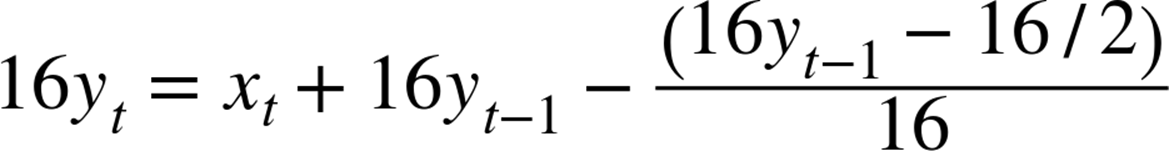
Everything is kept undivided as long as possible, and the average tracks the actual value very well, although we need to remember divide it back down by 16 before using it.

The only thing that’s a little odd about this expression is that the correction factor enters in with a negative sign, but that’s because we’re subtracting off the whole fractional part. The two negatives cancel out to make a positive and the value that we’re using for is rounded (correctly) up.

The Code

If you’ve hooked everything up right, you’ll have a vibration sensor hooked up to pin PC2 on the AVR. Now let’s flash in the code listed in Example 12-2 and use it.

Example 12-2. footstepDetector.c listing

/*

* Sensitive footstep-detector and EWMA demo

*/

// ------- Preamble -------- //

#include <avr/io.h>

#include <util/delay.h>

#include <avr/sleep.h>

#include "pinDefines.h"

#include "USART.h"

#define ON_TIME 2000 /* milliseconds */

#define CYCLE_DELAY 10 /* milliseconds */

#define INITIAL_PADDING 16 /* higher is less sensitive */

#define SWITCH PB7 /* Attach LED or switch relay here */

#define USE_POT 0 /* define to 1 if using potentiometer */

#if USE_POT

#define POT PC5 /* optional padding pot */

#endif

// -------- Functions --------- //

void initADC(void) {

ADMUX |= (1 << REFS0); /* reference voltage to AVCC */

ADCSRA |= (1 << ADPS1) | (1 << ADPS2); /* ADC clock prescaler /64 */

ADCSRA |= (1 << ADEN); /* enable ADC */

}

uint16_t readADC(uint8_t channel) {

ADMUX = (0b11110000 & ADMUX) | channel;

ADCSRA |= (1 << ADSC);

loop_until_bit_is_clear(ADCSRA, ADSC);

return (ADC);

}

int main(void) {

// -------- Inits --------- //

uint16_t lightsOutTimer = 0; /* timer for the switch */

uint16_t adcValue;

uint16_t middleValue = 511;

uint16_t highValue = 520;

uint16_t lowValue = 500;

uint16_t noiseVolume = 0;

uint8_t padding = INITIAL_PADDING;

LED_DDR = ((1 << LED0) | (1 << LED1) | (1 << SWITCH));

initADC();

initUSART();

// ------ Event loop ------ //

while (1) {

adcValue = readADC(PIEZO);

/* moving average -- tracks sensor's bias voltage */

middleValue = adcValue + middleValue - ((middleValue - 8) >> 4);

/* moving averages for positive and negative parts of signal */

if (adcValue > (middleValue >> 4)) {

highValue = adcValue + highValue - ((highValue - 8) >> 4);

}

if (adcValue < (middleValue >> 4)) {

lowValue = adcValue + lowValue - ((lowValue - 8) >> 4);

}

/* "padding" provides a minimum value for the noise volume */

noiseVolume = highValue - lowValue + padding;

/* Now check to see if ADC value above or below thresholds */

/* Comparison with >> 4 b/c EWMA is on different scale */

if (adcValue < ((middleValue - noiseVolume) >> 4)) {

LED_PORT = (1 << LED0) | (1 << SWITCH); /* one LED, switch */

lightsOutTimer = ON_TIME / CYCLE_DELAY; /* reset timer */

}

else if (adcValue > ((middleValue + noiseVolume) >> 4)) {

LED_PORT = (1 << LED1) | (1 << SWITCH); /* other LED, switch */

lightsOutTimer = ON_TIME / CYCLE_DELAY; /* reset timer */

}

else { /* Nothing seen, turn off lights */

LED_PORT &= ~(1 << LED0);

LED_PORT &= ~(1 << LED1); /* Both off */

if (lightsOutTimer > 0) { /* time left on timer */

lightsOutTimer--;

}

else { /* time's up */

LED_PORT &= ~(1 << SWITCH); /* turn switch off */

}

}

#if USE_POT /* optional padding potentiometer */

padding = readADC(POT) >> 4; /* scale down to useful range */

#endif

/* Serial output and delay */

/* ADC is 10-bits, recenter around 127 for display purposes */

transmitByte(adcValue - 512 + 127);

transmitByte((lowValue >> 4) - 512 + 127);

transmitByte((highValue >> 4) - 512 + 127);

_delay_ms(CYCLE_DELAY);

} /* End event loop */

return (0); /* This line is never reached */

}

Let’s start off with a look through the functions. initADC() and readADC() are general purpose functions that you can quite easily reuse in your code with a simple cut and paste. initADC() sets up the voltage reference, starts the ADC clock, and enables ADC.readADC() takes a channel value as an input, configures the multiplexer register to read from that channel, and then starts a conversion, waits, and returns the result. As you’ll see in the main loop, this makes calling multiple channels with the ADC as easy asresult = readADC(PIEZO); or result = readADC(ADC5);.

Rolling down to the main() function, we have the usual declarations for variables, and call the initialization functions, and then run the event loop.

Each cycle through the loop begins with an ADC read from the piezo channel, and then the code updates the middle value, and the high and low averages, respectively. To avoid round-off error, as is done in Equation 12-1, we’re not storing the moving-average values, but rather 16 times the moving-average value. Everywhere in the rest of the code where we use both the ADC reading directly and these smoothed versions, we have to remember to finish making the average by dividing by 16.

Notice that we only update the “moving average” for highValue when the measured ADC value is greater than the center value, and only update lowValue when it’s below. This way, highValue gives us the average value that’s above the middle, and lowValuegives us the average below it. The difference between these two is some measure of how wide the sampled waveform is on average. The value of this difference will track the average volume of background noise when there’s no active footsteps. As soon as we tap on the sensor, or step nearby it, the current value of the ADC will go very high or very low, but the average value will track this only slowly, and this is how we tell a real footstep from noise.

On top of this average measure of the background noise, I’ll add in an additional bit called padding. If you find that the sensor is triggering too often, or you’d just like it to only trigger on heavy-footed footsteps, you can use this value to add in some extra range in which the sensor won’t respond.

I’ve also left a define in the code (USE_POT) that you can enable if you’d like to hook up a potentiometer to PC5 and control the padding in real time. This makes the circuit easily tunable, and gives you an example of how easy it is to change values within your code via the ADC. When you define USE_POT to 1, the following two extra lines are inserted into the code:

#define POT PC5 /* optional padding pot */

padding = readADC(POT) >> 4; /* scale down to useful range */

and that’s enough to enable you to set the value of the variable padding by turning a knob. Neat, huh? Think back to every bit of code where we’ve defined a fixed value that you then had to edit, compile, flash, and test out. Why not add in a potentiometer and use an ADC channel to make the parameters adjustable in real time? When you’ve got the extra ADC channels and the extra processing time, nothing is stopping you.

The rest of the code just takes care of some display LEDs and the timing turning on and off the switch that controls the lights. Each time through the event loop, there’s a fixed delay at the very end. The switch only stays on for lightsOutTimer = ON_TIME / CYCLE_DELAY of these cycles after the last detected movement. But the sensor is looking for a new footstep with each cycle through the event loop, so as long as the vibrations continue, the switch’s timer variable will continue being reset to its maximum. The switch will turn off only after ON_TIME milliseconds of no activity.

I left these as defines because it’s interesting to play with them. If you sample the ADC too slowly (setting CYCLE_DELAY too large), you may miss the loud part of a footstep. If you sample too frequently, the sensitivity to background noise can increase. So you can play around with these values. The CYCLE_DELAY also implicitly sets the maximum time that the switch is on between footsteps; because lightsOutTimer is a 16-bit value, you’re “limited” to a maximum on-time of 655.36 seconds (about 11 minutes) with a 10 msCYCLE_DELAY.

The code also takes advantage of the two thresholds, one low and one high, to blink two separate LEDs, providing nice feedback as to how sensitive the circuit is. If only one of the LEDs blinks, your footstep was just above the noise threshold. If both blink and keep blinking back and forth for a second or so, you know that you’re detecting the footstep loud and clear.

By increasing the padding variable and making the sensor only react to larger values on the ADC, you could turn this circuit into a knock-detector suitable for detecting secret-knock patterns on a tabletop. For instance, if you want the AVR to do something only when you rap out the classic “shave-and-a-haircut” knock, you could keep track of the timing between detected knocks and only respond if they’re in the right approximate ratios.

If you increase the physical sensitivity of the sensor either mechanically by using a long lever arm and heavy weight or electronically by increasing the value of the bias resistors, this application will make a good seismometer. You might, for instance, store the values on a computer and look at them later. Or if you do a little preprocessing in the AVR and only record the values that are extreme, most likely in combination with some external storage, you can make yourself a capable logging seismometer.

Summary

In this chapter, you’ve learned two important techniques for getting either more accuracy (oversampling) or more stability (moving averaging) out of a digitized analog signal. Along the way, you learned two things about input conditioning: how to divide down a voltage to a manageable level for the AVR’s ADC using voltage dividers and how to handle an AC signal that doesn’t have a well-defined zero voltage reference.

In all of this, getting as much feedback from your measured system as possible is important. In the case of reasonably slow signals, you can send real-time data to your desktop computer over the serial port for simple diagnostics. For applications with very fast signals, nothing beats being able to hook up an oscilloscope to the circuit in question so that you can simply see how the voltages that you’re trying to measure are behaving.

The specifics of using any given analog sensor are usually very much application-dependent, so I hope that this chapter gives you enough of a basis to take the next steps yourself. And in the analog world, there’s really no substitute for building up your system and testing it out. This includes testing your circuit out in the environment that it’ll eventually be used in. No matter how well you think you’ve specified your sensors and your circuits, you’ll occasionally be surprised when they pick up on something in the environment that you hadn’t anticipated.

I built a noisemaker with light-dependent resistor light sensors once, wrote all of the firmware, and tested it out thoroughly, I thought. But I had tested it out in a room with strong daylight. As soon as I tried it out in a room with overhead fluorescent lights, there was a warbling noise overlaid on the pitch that I thought it should be playing. It turns out that the light sensors were reacting quickly enough to pick up the relatively quick light pulses that result from driving lights on 60 Hz AC house wiring. This took even longer to debug because it wasn’t simply a 60 Hz or 120 Hz pitch overlaid on top, but an interaction of the AVR’s sample rate with the 120 Hz bright-dark cycle from the lights. The solution was to take a moving average ADC value that smoothed out the fluorescent bulb’s light cycle, and all was well.

Grab yourself a sensor and hook it up to the AVR. See how it behaves, and then start coding up some neat interactions. But don’t get caught up in the idea that you can design everything from the specifications. With sensors, sometimes you’re going to be surprised by what they pick up, or don’t. So you’ve got to build it first, and then you can get down to puzzling out what’s really going on. And in my opinion, that’s more than half of the fun. Enjoy!