HTML5 Games: Creating Fun with HTML5, CSS3, and WebGL (2012)
part 3
Adding 3D and Sound
Chapter 11
Creating 3D Graphics with WebGL
in this chapter
• Introducing WebGL
• Using the OpenGL Shading Language
• Using Collada models
• Texturing and lighting 3D objects
• Creating a WebGL display module
You are already familiar with drawing 2D graphics with the canvas element. In this chapter, you expand that knowledge with 3D graphics and the WebGL context. I take you through enough of the WebGL API that you are able to render simple 3D scenes with lighting and textured objects.
In the first part of the chapter, I introduce you to the OpenGL Shading Language (GLSL), a language made specifically for rendering graphics with OpenGL. I then move on to show you step by step how to render simple 3D objects. You also see how to import the commonly used Collada model format into your WebGL applications.
Before wrapping up, I demonstrate how the techniques you’ve learned throughout the chapter can come together to create a WebGL version of the Jewel Warrior game display.
3D for the Web
The canvas element is designed so that the actual functionality is separate from the element. All graphics functionality is provided by a so-called context. In Chapter 6, you learned how to draw graphics on the canvas using a path-based API provided by the 2D context. WebGL extends thecanvas element with a 3D context.
WebGL is based on the OpenGL ES 2.0 graphics API, a variant of OpenGL aimed at embedded systems and mobile devices. This is also the version of OpenGL used for developing native applications on, for example, iPhone and Android devices. The WebGL specification is managed by the Khronos Group, which also oversees the various OpenGL specifications. Much of the WebGL specification is a straight mapping of the functionality in OpenGL ES. A big advantage of this is that guides, books, and sample code already exist that you can use for inspiration. Even if the context is not web related, OpenGL ES code examples in other languages such as C can still be valuable. You can also find plenty of GLSL code that can be plugged directly into WebGL applications.
Firefox has had WebGL support since version 4.0, Chrome since version 9, and Safari (OS X) since version 5.1. Safari’s WebGL is disabled by default but can be enabled in the developer menu, which is enabled in the Advanced section of the preferences. WebGL is also coming to Opera, but at the moment, it is available only in special test builds. Unfortunately, Microsoft has expressed concern over WebGL, claiming that security problems inherent in the design keep WebGL from living up to its standards. The result is that it is unlikely that Internet Explorer will see WebGL support in the near future. However, an independent project named IEWebGL aims at providing WebGL support via a plugin for Internet Explorer. The plugin is currently in beta testing, and you can read more about it on the website http://iewebgl.com/.
Support for WebGL on mobile devices is rather limited. The standard Android browser does support WebGL in any version currently available, although Mozilla has enabled WebGL in its mobile Firefox for Android. Apple is bringing WebGL to iOS with the release of iOS 5, but so far, it’s available only in its iAds framework. Web developers are left out in the cold on this one. We can only hope that later releases of iOS will expand this feature to the mobile Safari browser.
Getting started with WebGL
Most 3D graphics today, including what you see in this chapter, are based on objects made of small triangles, also called faces. Even very detailed 3D models with seemingly smooth surfaces reveal their polygonal nature when you zoom in close enough. Each triangle is described by three points, where each point, also called a vertex, is a three-dimensional vector. Put two triangles together to form a rectangle, put six squares together and you have a cube, and so on.
WebGL stores this 3D geometry in buffers that are uploaded to the graphics processing unit (GPU). The geometry is then rendered onto the screen, passing it through first a vertex shader and then a fragment shader. The vertex shader transforms the coordinates of the 3D points in accordance with the object’s rotation and position as well as the desired 2D projection. Finally, the fragment shader calculates the color values used to fill the projected triangles on the screen. Shaders are the first topic I discuss after this introductory section because they are fundamental to creating WebGL applications.
![]()
WebGL and OpenGL ES are much too complex to cover in full detail in a single chapter. If you are serious about WebGL development and OpenGL, I recommend spending time on web sites such as Learning WebGL (http://learningwebgl.com/) where you can find many tutorials and WebGL-related articles.
Because WebGL is based on canvas, the first step to using WebGL is to create a canvas element and grab a WebGL context object:
var canvas = document.createElement(“canvas”),
gl = canvas.getContext(“experimental-webgl”);
In the current implementations, the name of the context is experimental-webgl, but that will most likely change to webgl some time in the future as the implementations mature. The context object, gl, implements all the functionality of WebGL through various methods and constants.
Debugging WebGL
Debugging WebGL applications can be a bit tricky because most WebGL errors don’t trigger JavaScript errors. Instead, you must use the gl.getError() function to check whether an error has occurred. This function returns the value 0 if there are no errors or a WebGL error code indicating the type of error:
var error = gl.getError();
if (error != 0) {
alert(“An error occurred: “ + error);
}
Putting code like this after every WebGL function call causes both bloated code and a lot of extra work. To make debugging a bit easier and less cumbersome, the Chromium team put together a small helper library that lets you enable a special debug mode on a WebGL context object:
var gl = canvas.getContext(“webgl”);
gl = WebGLDebugUtils.makeDebugContext(gl);
When you use this debug context, the gl.getError() function is automatically called every time you call one of the WebGL functions. If an error occurs, gl.getError() translates the error code into a more meaningful text and throws a real JavaScript error. That makes it much easier to catch errors that might otherwise go unnoticed.
The debug helper is included in the code archive for this chapter and is also available at https://cvs.khronos.org/svn/repos/registry/trunk/public/webgl/sdk/debug/webgl-debug.js.
![]()
Enabling the debug mode adds extra function calls to all WebGL functions, which can have a negative effect on the performance of your application or game. Make sure you use the debug mode only during development and switch back to the plain WebGL context in production.
Creating a helper module
To simplify the implementation of Jewel Warrior’s WebGL display, you could put some of the more general WebGL functionality into a separate module. That’s just one good idea. For now, create a new module in webgl.js and start by adding the module definition as shown in Listing 11.1.
Listing 11.1 The Empty WebGL Helper Module
jewel.webgl = (function() {
return {
};
})();
As you progress through this chapter, you add more and more functions to the module.
![]()
I do not list the complete code for the examples and the WebGL display module. Doing so would involve a fair amount of repetition, and going over every detail would detract from the focus. You can find the full examples and code in the archive for this chapter.
Shaders
You need to know about two kinds of shaders: vertex shaders and fragment shaders. You can think of shaders as small programs used to instruct the GPU how to turn the data in the buffers into what you see rendered on the screen. Shaders are used to, for example, project points from 3D space to the 2D screen, calculate lighting effects, apply textures, and do many other things.
Shaders use a special language called OpenGL Shading Language (GLSL). As the name implies, this language is designed specifically for programming shaders for OpenGL. Other graphics frameworks use similar languages, such as DirectX and its High-Level Shading Language (HLSL). GLSL uses a C-like syntax, like JavaScript, so it shouldn’t be too difficult to grasp what is going on, even though you do need to learn a few new concepts.
For the most part, the syntax shouldn’t give you any trouble, but there are a few traps for developers who are mostly accustomed to JavaScript. One example is the lack of JavaScript’s automatic semicolon insertion. Semicolons are not optional in GLSL, and failing to add them at the end of lines causes errors.
Variables and data types
Variable declarations are similar to those in JavaScript but use the data type in place of the var keyword:
data_type variable_name;
As in JavaScript, you can also assign an initial value:
data_type variable_name = init_value;
GLSL introduces several data types not available in JavaScript. One data type that does behave the same in both JavaScript and GLSL is the Boolean type called bool:
bool mybool = true;
Besides bool, GLSL also has a few numeric types as well as several vector and matrix types.
Numeric types
Unlike JavaScript, GLSL has two numeric data types. Whereas all numbers in JavaScript use the number type, GLSL distinguishes between floating-point and integer values using the data types float and int, respectively.
Literal integer values can be written in decimal, octal, and hexadecimal form:
int mydec = 461; // decimal 461
int myoct = 0715; // octal 461
int myhex = 0x1CD; // hexadecimal 461
Literal floating-point values must either include a decimal point or an exponent part:
float myfloat = 165.843;
float myfloatexp = 43e-6; // 0.000043
GLSL cannot cast integer values to floating-point, so be careful to remember the decimal point in literal float values, even for values like 0.0 and 7.0.
Vectors
Vector types are used for many things in shaders. Everything from positions, normals, and colors is described using vectors. In GLSL, vector types come in three flavors: vec2, vec3, and vec4, where the number indicates the dimension of the vector. You create vectors as follows:
vec2 pos2d = vec3(3.42, 109.45);
vec3 pos3d = vec3(3.42, 109.45, 45.15);
You can also create vectors using other vectors in place of the components:
vec2 myXY = vec2(1.0, 2.0); // new two-dimensional vector
vec3 myXYZ = vec3(myXY, 3.0); // extend with a third dimension
This example combines the x and y components of the vec2 with a z value of 3.0 to create a new vec3 vector. This capability is useful for many things, for example, converting RGB color values to RGBA:
vec3 myColor = vec3(1.0, 0.0, 0.0); // red
float alpha = 0.5; // semi-transparent
vec4 myRGBA = vec4(myColor, alpha);
So far, all the vectors have been floating-point vectors. The vec2, vec3, and vec4 types allow only floating-point values. If you need vectors with integer values, you can use the ivec2, ivec3, and ivec4 types. Similarly, bvec2, bvec3, and bvec4 allow vectors with Boolean values. In most cases, you use only floating-point vectors.
Vector math
You can add and subtract vectors just as you would do float and int values. The addition is performed component wise:
vec2 v0 = vec2(0.5, 1.0);
vec2 v1 = vec2(1.5, 2.5);
vec2 v2 = v0 + v1; // = vec2(2.0, 3.5)
You can also add or subtract a single value to a vector:
float f = 7.0;
vec2 v0 = vec2(1.5, 2.5);
vec2 v1 = v0 + f; // = vec2(8.5, 9.5)
The float value is simply added to each component of the vector. The same applies to multiplication and division:
float f = 4.0;
vec2 v0 = vec2(3.0, 1.5);
vec2 v1 = v0 + f; // = vec2(12.0, 6.0)
If you use the multiplication operator on two vectors, the result is the dot product of the vectors:
vec2 v0 = vec2(3.5, 4.0);
vec2 v1 = vec2(2.0, 0.5);
vec2 v2 = v0 * v1; // = vec2(3.5 * 2.0, 4.0 * 0.5)
// = vec2(7.0, 2.0)
The dot product can also be calculated with the dot() function:
vec2 v2 = dot(v0, v1); // = vec2(7.0, 2.0)
The dot() function is just one of several functions that make life easier when you are working with vectors. Another useful example is the length() function, which calculates the length of a vector:
vec2 v0 = vec2(3.4, 5.2);
float len = length(v0); // = sqrt(3.4 * 3.4 + 5.2 * 5.2) = 6.21
Accessing vector components
The components of a vector are available via the properties x, y, z, and w on the vectors:
vec2 v = vec2(1.2, 7.3);
float x = v.x; // = 1.2
float y = v.y; // = 7.3
The properties r, g, b, and a are aliases of x, y, z, and w:
vec3 v = vec3(1.3, 2.4, 4.2);
float r = v.r; // = 1.3
float g = v.g; // = 2.4
float b = v.b; // = 4.2
A third option is to think of these components as a small array and access them with array subscripts:
vec2 v = vec2(1.2, 7.3);
float x = v[0]; // = 1.2
float y = v[1]; // = 7.3
Swizzling
A neat feature of GLSL vector types is swizzling. This feature enables you to extract multiple components of a vector and have them returned as a new vector. Suppose you have a three-dimensional vector and you want a two-dimensional vector with just the x and y values. Consider the following code:
vec3 myVec3 = vec3(1.0, 2.0, 3.0);
float x = myVec3.x; // = 1.0
float y = myVec3.y; // = 2.0
vec2 myVec2 = vec2(x, y);
This code snippet simply extracts the x and y components of vec3 to a couple of float variables that you can then use to, for example, create a new two-dimensional vector. This approach works just fine, but the following example achieves the same effect:
vec3 myVec3 = vec3(1.0, 2.0, 3.0);
vec2 myVec2 = myVec3.xy; // = vec2(1.0, 2.0)
Instead of just accessing the x and y properties of the vector, you can combine any of the components to create new vectors.
vec3 myVec3 = vec3(1.0, 2.0, 3.0);
myVec3.xy = vec2(9.5, 4.7); // myVec3 = vec3(9.5, 4.7, 3.0);
vec2 myVec2 = myVec3.zx; // = vec2(3.0, 9.5)
You can even use the same component multiple times in the same swizzle expression:
vec3 myVec3 = vec3(1.0, 2.0, 3.0);
vec2 myVec2 = myVec3.xx; // = vec2(1.0, 1.0)
The dimensions of the vector limit which components you can use. Trying to access, for example, the z component of a vec2 causes an error.
You can use both xyzw and rgba to swizzle the vector components:
vec4 myRGBA = vec4(1.0, 0.0, 0.0, 1.0);
vec3 myRGB = myRGBA.rgb; // = vec3(1.0, 0.0, 0.0)
You cannot mix the two sets, however. For example, myRGBA.xyga is not valid and produces an error.
Matrices
Matrices also have their own types, mat2, mat3, and mat4, which let you work with 2x2, 3x3, and 4x4 matrices. Only square matrices are supported. Matrices are initialized much like vectors by passing the initial values to the constructor:
mat2 myMat2 = mat2(
1.0, 2.0,
3.0, 4.0
);
mat3 myMat3 = mat3(
1.0, 2.0, 3.0,
4.0, 5.0, 6.0,
7.0, 8.0, 9.0
);
The columns of a matrix are available as vectors using a syntax similar to array subscripts:
vec3 row0 = myMat3[0]; // = vec3(1.0, 4.0, 7.0)
This syntax, in turn, lets you access individual components with syntax such as
float m12 = myMat3[1][2]; // = 8.0
Matrices can be added and subtracted, just like vectors and numbers:
mat2 m0 = mat2(
1.0, 5.7,
3.6, 2.1
);
mat2 m1 = mat2(
3.5, 2.0,
2.3, 4.0
);
mat2 m2 = m0 + m1; // = mat2(4.5, 7.7, 5.9, 6.1)
mat2 m3 = m0 - m1; // = mat2(-2.5, 3.7, 1.3, -1.9)
You can also multiply two matrices. This operation doesn’t operate component-wise but performs a real matrix multiplication. If you need component-wise matrix multiplication, you can use the matrixCompMult() function.
It is also possible to multiply a matrix and a vector with matching dimensions, producing a new vector:
vec2 v0 = vec2(2.5, 4.0);
mat2 m = mat2(
3.5, 7.0,
2.0, 5.0
);
vec v1 = v0 * m; // = vec2(
// m[0].x * v0.x + m[1].x * v0.y,
// m[0].y * v0.x + m[1].y * v0.y,
// )
// = vec2(36.75, 25.0)
Using shaders with WebGL
As mentioned earlier, the two types of shaders are vertex shaders and fragment shaders. You need one of each to render a 3D object. Vertex shaders and fragment shaders have the same basic structure:
declarations
void main(void) {
calculations
output_variable = output_value;
}
The declarations section declares any variables that the shader needs — both local variables and input variables coming from, for example, the vertex data. This section can also declare any helper functions utilized by the shader. Function declarations in GLSL look like this:
return_type function_name(parameters) {
...
}
This means that the function in the previous example is called main, has no return value, and takes no parameters. The main() function is required and is called automatically when the shader is executed. The shader ends by writing a value to an output variable. Vertex shaders write the transformed vertex position to a variable called gl_Position, and fragment shaders write the pixel color to gl_FragColor.
Vertex shaders
The vertex shader runs its code for each of the vertices in the buffer. Listing 11.2 shows a simple vertex shader.
Listing 11.2 A Basic Vertex Shader
attribute vec3 aVertex;
void main(void) {
gl_Position = vec4(aVertex, 1.0);
}
This simple shader declares an attribute variable called aVertex with the data type vec3, which is a vector type with three components. Attributes point to data passed from the WebGL application — in this case, the vertex buffer data. In this example, the vertex is converted to a four-dimensional vector and assigned, otherwise unaltered, to the output variable gl_Position. Later, you see how you can use view and projection matrices to transform the 3D geometry and add perspective.
Fragment shaders
Fragment shaders, also called pixel shaders, are similar to vertex shaders, but instead of vertices, fragment shaders operate on pixels on the screen. After the vertex shader processes the three points in a triangle and transforms them to screen coordinates, the fragment shader colorizes the pixels in that area. Listing 11.3 shows a simple fragment shader.
Listing 11.3 A Basic Fragment Shader
#ifdef GL_ES
precision mediump float;
#endif
void main(void) {
gl_FragColor = vec4(1.0, 0.0, 0.0, 1.0);
}
The output variable in fragment shaders is a vec4 called gl_FragColor. This example just sets the fragment color to a non-transparent red.
![]()
The term fragment refers to the piece of data that potentially ends up as a pixel if it passes depth testing and other requirements. A fragment does not need to be the size of a pixel. Fragments along edges, for example, could be smaller than a full pixel. Despite these differences, the terms fragment and pixel, as well as fragment shader and pixel shader, are often used interchangeably.
You are probably wondering about the first three lines in Listing 11.3. The OpenGL ES version of GLSL requires that fragment shaders specify the precision of float values. Three precisions are available: lowp, mediump, and highp. You can give each float variable a precision by putting one of the precision qualifiers in front of the declaration:
mediump float myfloatvariable;
You can also specify a default precision by adding a precision statement at the top of the shader code:
precision mediump float;
Earlier versions of desktop OpenGL do not support the precision keyword, though, and using it risks causing errors. However, GLSL supports a number of preprocessor statements such as #if, #ifdef, and #endif. You can use these statements to make sure a block of code is compiled only under certain conditions:
#ifdef GL_ES
precision highp float;
#endif
This example causes the precision code to be ignored if GL_ES is not defined, which it is only in GLSL ES.
Including shader code in JavaScript
Getting the GLSL source code into your WebGL application can be a bit tricky. The browser doesn’t understand GLSL, but you can still include the code in a script element directly in the HTML. Just give it a custom script type so the browser doesn’t attempt to interpret the code as JavaScript:
<script id=”fragment” type=”x-shader/x-fragment”>
... // GLSL source code
</script>
You can then extract the contents of the script element with standard DOM scripting. Note, however, that you can’t reference an external GLSL file by adding an src attribute to the script element because the browser doesn’t download scripts it can’t execute.
Another option is to pack the GLSL in a string literal and embed it in the JavaScript code:
var fsource =
“#ifdef GL_ES\r\n” +
” precision highp float;\r\n” +
“#endif\r\n” +
“void main(void) {\r\n” +
“ gl_FragColor = vec4(0.7, 1.0, 0.8, 1.0); \r\n” +
“}\r\n”;
You can add \r\n at the end of each line to include line breaks in the source. Otherwise, the source code is concatenated to a single line, making it harder to debug because shader error messages include line numbers. This is the method I chose to use in the examples included in the code archive for this chapter. It may not be the prettiest solution, but it gets the job done. For the sake of readability, the code listings in the rest of this chapter show the GLSL code without quotation marks and newline characters.
A third option is to load the shader code from separate files with Ajax. Although this approach adds extra HTTP requests, it has the advantage of storing the GLSL as is and encourages reuse of the shader files.
Creating shader objects
The shader source needs to be loaded into a shader object and compiled before you can use it. Use the gl.createShader() method to create shader objects:
var shader = gl.createShader(shaderType);
The shader type can be either gl.VERTEX_SHADER or gl.FRAGMENT_SHADER. The rest of the process for creating shader objects is the same regardless of the shader type.
You specify the GLSL source for the shader object with the gl.shaderSource() method. When the source is loaded, you can compile it with the gl.compileShader() method:
gl.shaderSource(shader, source);
gl.compileShader(shader);
You don’t get any JavaScript errors if the compiler fails because of bad GLSL code, but you can check for compiler errors by looking at the value of the gl.COMPILE_STATUS parameter:
if (!gl.getShaderParameter(shader, gl.COMPILE_STATUS)) {
throw gl.getShaderInfoLog(shader);
}
The value of the gl.COMPILE_STATUS is true if no compiler errors occurred. If there were errors, you can use the gl.getShaderInfoLog() method to get the relevant error message. If you want to test this error-catching check, you can just add some invalid GLSL code to your shader source.
Listing 11.4 shows these calls combined to form the first function for the WebGL helper module.
Listing 11.4 Creating Shader Objects
jewel.webgl = (function() {
function createShaderObject(gl, shaderType, source) {
var shader = gl.createShader(shaderType);
gl.shaderSource(shader, source);
gl.compileShader(shader);
if (!gl.getShaderParameter(shader, gl.COMPILE_STATUS)) {
throw gl.getShaderInfoLog(shader);
}
return shader;
}
return {
createShaderObject : createShaderObject
}
})();
Creating program objects
After both shaders are compiled, they must be attached to a program object. Program objects join a vertex shader and fragment shader to form an executable that can run on the GPU. Create a new program object with the gl.createProgram() method:
var program = gl.createProgram();
Now attach the two shader objects:
gl.attachShader(program, vshader);
gl.attachShader(program, fshader);
Finally, the program must be linked:
gl.linkProgram(program);
As with the shader compiler, you need to check for linker errors manually. Examine the gl.LINK_STATUS parameter on the program object and throw a JavaScript error if necessary:
if (!gl.getProgramParameter(program, gl.LINK_STATUS)) {
throw gl.getProgramInfoLog(program);
}
Listing 11.5 shows these function calls combined to form the createProgramObject() function for the WebGL helper module.
Listing 11.5 Creating Program Objects
jewel.webgl = (function() {
...
function createProgramObject(gl, vs, fs) {
var program = gl.createProgram();
gl.attachShader(program, vs);
gl.attachShader(program, fs);
gl.linkProgram(program);
if (!gl.getProgramParameter(program, gl.LINK_STATUS)) {
throw gl.getProgramInfoLog(program);
}
return program;
}
return {
createProgramObject : createProgramObject,
...
}
})();
The shaders and program object are now ready for use:
gl.useProgram(program);
The program is now enabled and set as the active shader program. If you use more than one program to render different objects, make sure you call gl.useProgram() to tell WebGL to switch programs.
Any attribute variables in the vertex shader must be enabled before they can be used. On the JavaScript side of WebGL, you refer to an attribute variable by its location, which you can get with the gl.getAttribLocation() function:
var aVertex = gl.getAttribLocation(program, “aVertex”);
You can now enable the attribute:
gl.enableVertexAttribArray(aVertex);
Uniform variables
If you need to set values that are global to the entire group of vertices or pixels currently being rendered, you can use uniform variables. The value of a uniform variable is set with JavaScript and doesn’t change until you assign a new value. Listing 11.6 shows a fragment shader with a uniform value.
Listing 11.6 A Fragment Shader with a Uniform Variable
#ifdef GL_ES
precision highp float;
#endif
uniform vec4 uColor;
void main(void) {
gl_FragColor = uColor;
}
Just add the uniform keyword to the variable declaration to make it a uniform variable. Because the value is set on the JavaScript side of WebGL, you cannot write to these variables from within the shader.
Uniform variables are referenced by their location in the same way as attribute variables. Use the gl.getUniformLocation() function to get the location:
var location = gl.getUniformLocation(program, “uColor”);
The function you need to call to update a uniform variable depends on the data type of the variable. No fewer than 19 functions exist that update uniform variables, so picking the right one might seem a bit daunting at first.
To update a single float or vector variable, you can use functions of the form uniform[1234]f(). For example, if loc is the location of a uniform vec2, the following updates the value to vec2(2.4, 3.2):
gl.uniform2f(location, 2.4, 3.2);
For arrays, you can use functions of the form uniform[1234]fv(). For example, the following updates an array of three vec2 values:
gl.uniform2fv(location, [
2.4, 3.6,
1.6, 2.0,
9.2, 3.4
]);
The uniform[1234]i() and uniform[1234]fv() forms allow you to update integer values.
Matrix values are set with the functions of the form uniformMatrix[234]fv():
gl.uniformMatrix3fv(location, false, [
4.3, 6.5, 1.2,
2.3, 7.4, 0.9,
5.5, 4.2, 3.0
]);
The second parameter specifies whether the matrix values should be transposed. This capability is not supported, however, and the argument must always be set to false. You can pass the matrix values as a regular JavaScript array or as a Float32Array typed array object.
Returning to the fragment color, the uColor uniform value is vec4, so you can set this value with gl.uniform4f() or gl.uniform4fv():
gl.uniform4f(location, 0.5, 0.5, 0.5, 1.0); // 50% gray
gl.uniform4fv(location, [1.0, 0.0, 1.0, 1.0]); // magenta
Varying variables
In addition to uniforms and local variables, you can have varying variables that carry over from the vertex shader to the fragment shader. Consider a triangle in 3D space. The vertex shader does its work on all three vertices of the triangle before the fragment shader takes over and processes the pixels that make up the triangle. When the varying variable is read in the fragment shader, its value varies depending on where the pixel is located on the triangle. Listing 11.7 shows an example of a varying variable used in the vertex shader.
Listing 11.7 Vertex Shader with Varying Variable
attribute vec3 aVertex;
varying vec4 vColor;
void main(void) {
gl_Position = vec4(aVertex, 1.0);
vColor = vec4(aVertex.xyz / 2.0 + 0.5, 1.0);
}
In the example in Listing 11.7, the position of the vertex determines the color value assigned to the vColor variable. The variable is declared as varying, making it accessible in the fragment shader as shown in Listing 11.8.
Listing 11.8 Fragment Shader with Varying Variable
#ifdef GL_ES
precision highp float;
#endif
varying vec4 vColor;
void main(void) {
gl_FragColor = vColor;
}
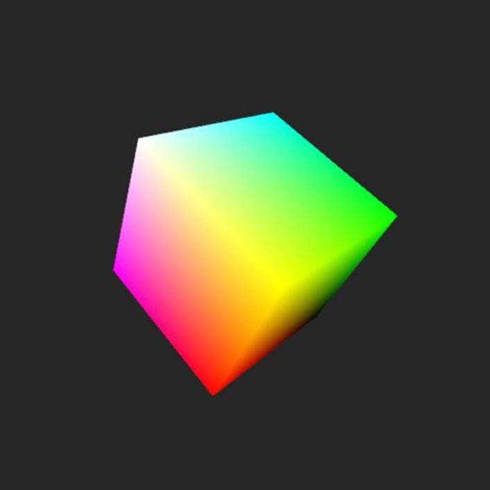
Because different colors were assigned to the vertices, the result is a smooth gradient across the triangle.
![]()
Not all data types are equal when it comes to varying variables. Only float and the floating-point vector and matrix types can be declared as varying.
Rendering 3D Objects
Now that you have some basic knowledge about how shaders work in WebGL, it’s time to move forward to constructing and rendering some simple 3D objects. Most applications have some setup code and a render cycle that continuously updates the rendered image.
The amount of setup code depends entirely on the nature of the application and the amount of 3D geometry and shaders. A few things almost always need to be taken care of, however. One example is the clear color, which is the color to which the canvas is reset whenever it is cleared. You can set this color with the gl.clearColor() method:
gl.clearColor(0.15, 0.15, 0.15, 1.0);
The gl.clearColor() method takes four parameters, one for each of the red, green, blue, and alpha channels. WebGL always works with color values from 0 to 1. Usually, you should also enable depth testing:
gl.enable(gl.DEPTH_TEST);
This method makes WebGL compare the distances between the objects and the point of view so that elements that are farther away don’t appear in front of closer objects. The argument passed to gl.enable(), gl.DEPTH_TEST, is a constant numeric value. WebGL has many of these constants, but you see only a small subset of them throughout this chapter. Some of the constants are capabilities that you can toggle on and off with the gl.enable() and gl.disable() methods, whereas others are parameters that you can query with the function gl.getParameter(). You can, for example, query the clear color with the COLOR_CLEAR_VALUE parameter:
var color = gl.getParameter(gl.COLOR_CLEAR_VALUE);
The type of the return value depends on the parameter; in the case of gl.COLOR_CLEAR_VALUE, the return value is a Float32Array with four numerical elements, corresponding to the RGBA values of the clear color.
Using vertex buffers
WebGL uses buffer objects to store vertex data. You load the buffer with values, and when you tell WebGL to render the 3D content, the data is loaded to the GPU. Any time you want to change the vertex data, you must load new values into the buffer. You create buffer objects with thegl.createBuffer() function:
var buffer = gl.createBuffer();
gl.bindBuffer(gl.ARRAY_BUFFER, buffer);
The gl.bindBuffer() function binds the buffer object to the gl.ARRAY_BUFFER target, telling WebGL to use the buffer as a vertex buffer.
gl.bufferData(
gl.ARRAY_BUFFER, data, gl.STATIC_DRAW
);
Notice that the buffer object isn’t passed to the gl.bufferData() function. Instead, the function acts on the buffer currently bound to the target specified in the first argument.
The third parameter specifies how the buffer is used in terms of how often the data is updated and accessed. The three available values are gl.STATIC_DRAW, gl.DYNAMIC_DRAW, and gl.STREAM_DRAW. The gl.STATIC_DRAW value is appropriate for data loaded once and drawn many times,gl.DYNAMIC_DRAW is for repeated updates and access, and gl.STREAM_DRAW should be used when the data is loaded once and drawn only a few times.
The data should be passed to gl.bufferData() as a Float32Array typed array object. This process is generic enough that you can add it to the webgl.js helper module. Listing 11.9 shows the gl.createFloatBuffer() function.
Listing 11.9 Creating Floating-point Buffers
jewel.webgl = (function() {
...
function createFloatBuffer(gl, data) {
var buffer = gl.createBuffer();
gl.bindBuffer(gl.ARRAY_BUFFER, buffer);
gl.bufferData(gl.ARRAY_BUFFER,
new Float32Array(data), gl.STATIC_DRAW
);
return buffer;
}
return {
createFloatBuffer : createFloatBuffer,
...
}
})();
You can then use the function to create a buffer object from an array of coordinates:
var vbo = webgl.createFloatBuffer(gl, [
-0.5, -0.5, 0.0, // triangle 1, vertex 1
0.5, -0.5, 0.0, // triangle 1, vertex 2
0.5, 0.5, 0.0, // triangle 1, vertex 3
-0.5, -0.5, 0.0, // triangle 2, vertex 1
0.5, 0.5, 0.0, // triangle 2, vertex 2
-0.5, 0.5, 0.0 // triangle 2, vertex 3
]);
This code snippet creates the vertex data necessary to render a two-dimensional square.
Using index buffers
If you look at the vertices in the preceding example, you can see that some of the vertices are duplicated. The vertex buffer is created with six vertices when only four are really needed to make a square.
var vbo = webgl.createFloatBuffer(gl, [
-0.5, -0.5, 0.0,
0.5, -0.5, 0.0,
0.5, 0.5, 0.0,
-0.5, 0.5, 0.0
]);
You then need to declare how these vertices are used to create the triangles. You do this with an index buffer, which is basically a list of indices into the vertex list that describes which vertices belong together. Each three entries in the index buffer make up a triangle. The index buffer is created in a way similar to the vertex buffer, as Listing 11.10 shows.
Listing 11.10 Creating Index Buffers
jewel.webgl = (function() {
...
function createIndexBuffer(gl, data) {
var buffer = gl.createBuffer();
gl.bindBuffer(gl.ELEMENT_ARRAY_BUFFER, buffer);
gl.bufferData(
gl.ELEMENT_ARRAY_BUFFER,
new Uint16Array(data), gl.STATIC_DRAW
);
return {
return buffer;
}
}
return {
createIndexBuffer : createIndexBuffer,
...
}
})();
The important differences here are that the buffer is initialized with the type gl.ELEMENT_ARRAY_BUFFER and that the buffer uses integer data instead of floating-point values. The index buffer for the four vertices can now be created as follows:
var ibo = webgl.createIndexBuffer(gl, [
0, 1, 2,
0, 2, 3
]);
Using models, views, and projections
Simply defining the model data is not enough to render it in any meaningful way. You also need to transform the vertices so that the object is rendered at the desired position in the world with the desired rotation. The coordinates in the vertex data are all relative to the object’s own center, so if you want to position the object 5 units above the (x, z) plane, you add 5 to the y component of all vertices. If the viewer is located in any other position than (0,0,0), that location would also have to be subtracted from the vertex position. Any rotation of both the viewer and the object itself must also be taken into account.
What if those values change, though? You could re-transform the vertex data and send it to the GPU again, but transferring vertex data from JavaScript to the GPU is relatively expensive in terms of resources and can potentially slow down your application. Instead of updating the vertex buffer in each render cycle, the transformation task is usually delegated to the vertex shader. To transform the vertices into screen coordinates, you need to construct two matrices: the model-view matrix and projection matrix. The model-view matrix describes the transformations needed to bring a vertex into the correct position relative to the viewer. The projection matrix describes how to project the transformed points onto the 2D screen. The matrices can be declared as uniform variables in the shaders, so you just need to update those in each cycle.
Working with vectors and matrices in JavaScript is not trivial because there is no built-in support for either. However, available libraries provide the most common operations and save you from all the details of matrix manipulation and linear algebra. My matrix library of choice is glMatrix, a library that was developed specifically with WebGL in mind and is, to quote the developer, “stupidly fast.” You can read more about glMatrix at http://code.google.com/p/glmatrix/. I also included the library in the code archive for this chapter.
The model-view matrix
Let’s start with the model-view matrix. The glMatrix library provides its functionality through static methods on the three objects: vec3, mat3, and mat4. Creating a 4x4 matrix is as easy as
var mvMatrix = mat4.create();
Use the mat4.identity() method to set the matrix to the identity matrix (all zeros with a diagonal of ones).
mat4.identity(mvMatrix);
// = 1 0 0 0
// 0 1 0 0
// 0 0 1 0
// 0 0 0 1
To move the position, use the mat4.translate() method:
mat4.translate(mvMatrix, [0, 0, -5]);
The second parameter of the mat4.translate() method is the vector that will be added to the object’s position. Whether you do two translations — one for the object position and one for the view position — or you combine them is up to you. Notice that vectors are just regular JavaScript arrays; the same is true for matrices. Part of what makes glMatrix efficient is that it keeps things simple and doesn’t create a lot of custom objects.
The mat4.rotate() method adds rotation around a specified axis:
mat4.rotate(mvMatrix, Math.PI / 4, [0, 1, 0]);
The second parameter is the amount of rotation, specified in radians. The third parameter is the axis around which the object will be rotated. Any vector does the job here.
You can combine the operations to a setModelView() function for the webgl.js helper module, as Listing 11.11 shows.
Listing 11.11 Setting the Model-view Matrix
jewel.webgl = (function() {
...
function setModelView(gl, prgm, pos, rot, axis) {
var mvMatrix = mat4.identity(mat4.create());
mat4.translate(mvMatrix, pos);
mat4.rotate(mvMatrix, rot, axis);
gl.uniformMatrix4fv(
gl.getUniformLocation(prgm, “uModelView”),
false, mvMatrix
);
return mvMatrix;
}
...
})();
After you apply the translation and rotation to the model-view matrix, the matrix is updated in the shaders with the gl.uniformMatrix4fv() function. The model-view function assumes that the uniform in the shader is called uModelView.
The projection matrix
There is more than one way to project a 3D point to a 2D surface. One often-used method is perspective projection where objects that are far away appear smaller than closer objects, simulating what the human eye sees. The glMatrix library actually has a function for creating a perspective projection matrix:
var projMatrix = mat4.create();
mat4.perspective(fov, aspect, near, far, projMatrix);
The fov parameter is the field-of-view (FOV) value, an angular measurement of how much the viewer can see. This value is given in degrees and specifies the vertical range of the FOV. Humans normally have a vertical FOV of around 100 degrees, but games often use a lower number than that. Values between 45 and 90 degrees are commonly used, but the perfect value is subjective and depends on the needs of the game.
The aspect parameter is the aspect ratio of the output surface. In most cases, you should use the width to height ratio of the output canvas. The near and far parameters specify the boundaries of the view area. Anything closer to the viewer than near or farther away than far is not rendered.
The helper function for the projection matrix is shown in Listing 11.12.
Listing 11.12 Projection Matrix Helper Function
jewel.webgl = (function() {
...
function setProjection(gl, prgm, fov, aspect, near, far) {
var projMatrix = mat4.create();
mat4.perspective(
fov, aspect,
near, far,
projMatrix
);
gl.uniformMatrix4fv(
gl.getUniformLocation(prgm, “uProjection”),
false, projMatrix
);
return projMatrix;
}
...
})();
Matrices in the vertex shader
To use the two matrices in the vertex shader, you can add the uniform declarations for uModelView and uProjection:
uniform mat4 uModelView;
uniform mat4 uProjection;
To transform the vertex position, simply multiply it with both matrices. Because they are 4x4 matrices, you need to turn the vertex into vec4 before multiplying. Listing 11.13 shows the complete vertex shader.
Listing 11.13 Transforming the Vertex Position
attribute vec3 aVertex;
uniform mat4 uModelView;
uniform mat4 uProjection;
varying vec4 vColor;
void main(void) {
gl_Position = uProjection * uModelView * vec4(aVertex, 1.0);
vColor = vec4((aVertex.xyz + 1.0) / 2.0, 1.0);
}
Rendering
Often, it’s not enough to just set the model-view and projection matrices once in the beginning of the application. If the object is animated — for example, if it’s moving or rotating — the model-view must be continuously updated. In Chapter 9, I showed you how to make simple animation cycles with the requestAnimationFrame() timing function. You can use the same technique to create a rendering cycle for WebGL. An example of a cycle function is shown in Listing 11.14.
Listing 11.14 The Rendering Cycle
function cycle() {
var rotation = Date.now() / 1000,
axis = [0, 1, 0.5],
position = [0, 0, -5];
webgl.setModelView(gl, program, position, rotation, axis);
draw();
requestAnimationFrame(cycle);
}
In this example, the model-view matrix is updated each frame to adjust the rotation. The rotation applied to the matrix is based on the current time, so the object will rotate at an even rate, regardless of how often the cycle runs. After you update the model-view, a draw() function, or something similar, could take care of rendering the object. An initial cycle() call sets things in motion.
Clearing the canvas
The cycle() function in Listing 11.14 calls a draw() function to do the actual rendering. The first thing this function should do before rendering anything is clear the canvas. You do this with the gl.clear() function:
gl.clear(mask);
This function takes a single parameter that specifies what it should clear. Possible values that you can use are the constants gl.COLOR_BUFFER_BIT, gl.DEPTH_BUFFER_BIT, and gl.STENCIL_BUFFER_BIT. These values refer to the three buffers (color, depth, and stencil) that have become standard in modern graphics programming. The color buffer contains the actual pixels rendered to the canvas and what you can see on the screen. The depth buffer is used to keep track of the depth of each pixel when drawing overlapping elements at different distances from the viewpoint. The third buffer, the stencil buffer, is essentially a mask applied to the rendered content. It can be useful for shadow effects, for example.
The mask parameter is a bit-mask. Bit-masks provide a resource-efficient way to specify multiple on/off values in a single numeric value. Each gl.*_BUFFER_BIT value corresponds to a different bit in the number. This way, you can pass more than one value to the function by using the bitwiseOR (pipe) operator to combine values:
gl.clear(gl.COLOR_BUFFER_BIT | gl.DEPTH_BUFFER_BIT);
This function clears both the color buffer and depth buffer. The color of the canvas is reset to the color set with the gl.clearColor() function, as I showed you at the beginning of this chapter.
Next, you need to declare the viewport, which is the rectangular area of the canvas where the rendered content is placed:
gl.viewport(0, 0, canvas.width, canvas.height);
You don’t actually need to set this in each render cycle, but if the dimensions of the canvas element change after you set the viewport, the viewport is not automatically updated. Setting the viewport in each cycle ensures that the viewport is set to the full canvas area before anything is rendered.
Drawing the vertex data
Now we’re ready to draw some shapes. Before the vertex data is available to the vertex shader through the aVertex attribute, you must activate the vertex buffer. First, make sure the vertex buffer is bound to the gl.ARRAY_BUFFER target:
gl.bindBuffer(gl.ARRAY_BUFFER, vbo);
You can now assign the buffer data to the attribute value with the gl.vertexAttribPointer() function:
gl.vertexAttribPointer(aVertex, 3, gl.FLOAT, false, 0, 0);
This function assigns the currently bound buffer to the attribute variable identified by aVertex, which is an attribute location retrieved with gl.getAttribLocation().The five remaining parameters are as follows: attribute size, data type, normalized, stride, and offset. The attribute size is the number of components of each vector; in this case, each vertex has three components. The data type refers to the data type of the vertex components. Note, however, that the values are converted to float regardless of the data type. The normalized parameter is used only for integer data. If it is set to true, the components are normalized to the range [-1,1] for signed values or [0,1] for unsigned values. The stride is the number of bytes from the start of one vertex to the start of the next. If you specify a stride value of 0, WebGL assumes that vertices are tightly packed and there are no gaps in the data. The last parameter specifies the position of the first vertex.
That’s it for the vertices — on to the index buffer, which just needs to be bound to the gl.ELEMENT_ARRAY_BUFFER target:
gl.bindBuffer(gl.ELEMENT_ARRAY_BUFFER, ibo);
This tells WebGL to use the buffer as indices instead of as vertex data. You can now draw the triangles with the gl.drawElements() function:
gl.drawElements(gl.TRIANGLES, num, gl.UNSIGNED_SHORT, 0);
The gl.drawElements() function takes four arguments: the rendering mode, number of elements, data type of the values, and offset at which to start. The gl.TRIANGLES mode tells WebGL that a new triangle starts after every three index values. The data type corresponds to the type of the values used to create the buffer data. The index buffer was created from a Uint16Array() typed array, which corresponds to the gl.UNSIGNED_SHORT value in WebGL. Unless you are rendering only a subset of the triangles, the offset parameter should be set to zero.
Combine these calls and you get a draw() function like the one shown in Listing 11.15.
Listing 11.15 Drawing the Object
function draw() {
gl.clear(gl.COLOR_BUFFER_BIT | gl.DEPTH_BUFFER_BIT);
gl.viewport(0, 0, canvas.width, canvas.height);
gl.bindBuffer(gl.ARRAY_BUFFER, geometry.vbo);
gl.vertexAttribPointer(aVertex, 3, gl.FLOAT, false, 0, 0);
gl.bindBuffer(gl.ELEMENT_ARRAY_BUFFER, geometry.ibo);
gl.drawElements(
gl.TRIANGLES, geometry.num, gl.UNSIGNED_SHORT, 0
);
}
In the file 01-cube.html, you can find an example of how to use the techniques shown here to render a colored, rotating cube, as seen in Figure 11-1.
Figure 11-1: Rendering a colored cube
Other rendering modes
Rendering modes other than gl.TRIANGLES are available. WebGL can also render points and lines, and it has modes that interpret the vertex data in different ways. The available rendering modes are
• TRIANGLES
• TRIANGLE_STRIP
• TRIANGLE_FAN
• POINTS
• LINES
• LINE_LOOP
• LINE_STRIP
I don’t go into detail on all these modes here, but I encourage you to play around with them. A mode like gl.TRIANGLE_STRIP is especially useful because it allows you to decrease the number of indices needed if you order the triangles so the next triangle starts where the previous triangle ended. Another interesting mode is gl.POINTS, which is great for things such as particle effects, and gl.LINES mode, which you can use to render lines and wireframe-like objects.
In the previous example, WebGL needed a list of indices to be able to construct the triangles from the vertices. If the vertex data is packed so the vertices can be read from start to finish, you don’t need the index data but can instead use the gl.drawArrays() function to render the geometry:
var vbo = createFloatBuffer([
-0.5, -0.5, 0.0, // tri 1 ver 1
0.5, -0.5, 0.0, // tri 1 ver 2
0.5, 0.5, 0.0, // tri 1 ver 3 / tri 2 ver 1
-0.5, 0.5, 0.0, // tri 2 ver 2
-0.5, -0.5, 0.0 // tri 2 ver 3
]);
gl.drawArrays(gl.TRIANGLE_STRIP, 0, 5);
This example sets up the vertices needed to render a square as a triangle strip. Notice that the third vertex is used both as the third vertex in the first triangle and as the first vertex in the second triangle.
Loading Collada models
Specifying all the vertex and index values manually is feasible only for simple shapes, such as cubes, planes, or other basic primitives. Any sort of complex object that requires many triangles is better imported from external files. Be aware that 3D model formats are a dime a dozen, but only a few are easily parsed by JavaScript. The ideal solution would be JSON-based format, but I have yet to come across such a format supported in the major graphics applications.
XML, however, is also pretty easy to use in JavaScript because it can be parsed using the built-in DOM API. Collada is an XML-based model format maintained by the Khronos Group, the same group responsible for WebGL. The format has gained a lot of popularity in recent years, and many 3D modeling applications can export their models as Collada files.
If you’re new to 3D modeling and don’t feel like shelling out hundreds or even thousands of dollars for a 3D graphics application, I recommend you try out Blender (www.blender.org/), a free and open-source 3D graphics package. It is available on several platforms, including Windows, Mac OSX, and Linux, and it has a feature set comparable to those found in many commercial applications. It also supports export and import of a variety of file formats, including Collada.
Fetching the model file
First, you need to load the model data, but you can easily take care of that with a bit of Ajax. The webgl.loadModel() function in Listing 11.16 shows the standard Ajax code needed to load a model file.
Listing 11.16 Loading the XML File
jewel.webgl = (function() {
...
function loadModel(gl, file, callback) {
var xhr = new XMLHttpRequest();
xhr.open(“GET”, file, true);
// override mime type to make sure it’s loaded as XML
xhr.overrideMimeType(“text/xml”);
xhr.onreadystatechange = function() {
if (xhr.readyState == 4) {
if (xhr.status == 200 && xhr.responseXML) {
callback(parseCollada(gl, xhr.responseXML));
}
}
}
xhr.send(null);
}
return {
...
loadModel : loadModel
};
})();
When the file finishes loading, the XML document is available in the responseXML property of xhr. This document is passed on to a webgl.parseCollada()function, which must parse the XML document and create the necessary buffer objects.
Parsing the XML data
The parseCollada() function can use Sizzle to extract the relevant nodes, and from there, it’s a matter of constructing arrays with the values. I don’t go into details of the Collada XML format and the parseCollada() function but instead refer you to the Collada specification, available atwww.khronos.org/collada/. You can find the full parsing function in the webgl.js module in the code archive for this chapter, but please note that it implements a very small subset of the format to get the test model loaded. Listing 11.17 shows the return value from the parsing function.
Listing 11.17 Parsing Collada XML Data
jewel.webgl = (function() {
...
function parseCollada(xml) {
... // XML parsing
return {
vbo : createFloatBuffer(gl, vertices),
nbo : createFloatBuffer(gl, normals),
ibo : createIndexBuffer(gl, indices),
num : indices.length
};
}
...
})();
The return value of webgl.parseCollada()is a small object with the three buffer objects vbo, nbo, and ibo, as well as a number indicating the number of indices. The vbo and ibo buffers contain the vertex and index data; the third buffer, nbo, contains the normal vectors. You see how these normal vectors are used in the next section when I show you how to enhance the rendering with textures and lighting effects. The example in the file 02-collada.html uses the Collada loading code to load and render a model of a sphere. The resulting image is shown in Figure 11-2.
Figure 11-2: Rendering the Collada sphere model
![]()
You cannot access local files with Ajax requests. This example needs to run from a web server in order to work.
Using Textures and Lighting
The two examples you’ve seen so far have been a bit bland and flat. To really bring out the third dimension in the image, the scene needs lighting. The color scheme of the surface isn’t very interesting either. In many cases, the surface should be covered by a texture image to simulate a certain material. First, however, let’s look at the lighting issue.
Adding light
You can use many different methods to apply lighting to a 3D scene, ranging from relatively simple approximations to realistic but complex mathematical models. I stick to a simple solution called Phong lighting, which is a common approximation of light reflecting off a surface.
The Phong model applies light to a point on a surface by using three different components: ambient, diffuse, and specular light. Ambient light simulates the scattering of light from the surrounding environment — that is, light that doesn’t hit the point directly from the source but bounces off other objects in the vicinity. Diffuse light is the large, soft highlight on the surface that appears when light coming directly from the light source hits the surface. This light component simulates the diffuse reflection that happens when the surface reflects incoming light in many different directions. Specular light depends on the position of the viewer and simulates the small intense highlights that appear when light reflects off the surface directly toward the eye. The color of a surface point is then determined as the surface color multiplied by the sum of the three lighting components:
gl_FragColor = color * (ambient + diffuse + specular);
The ambient component is the easiest to implement because it is simply a constant. The diffuse and specular components require a bit of trigonometry, however.
Angles and normals
The diffuse light component uses the angle between the light ray hitting the object’s surface and the surface normal. The normal to a point on the surface is a vector that is perpendicular to the surface at that point. For example, a surface that is parallel to the ground has a normal vector that points straight up. Normal vectors are normalized, so the norm, or length, of the vector is exactly 1:
length = sqrt(v.x * v.x + v.y * v.y + v.z * v.z) = 1.0
This is also called the unit length, and a vector with unit length — for example, a normal vector — is called a unit vector.
Because the 3D geometry is made of triangles and vertices and not smoothly curved surfaces, the normals are actually vertex normals in the sense that each vertex has a normal perpendicular to a plane tangent at that vertex position. The Collada loading function shown earlier already creates a normal buffer object with the normal data found in the model file.
In the vertex shader, you access the vertex normals through an attribute variable, just as you access the vertices themselves:
attribute vec3 aNormal;
The normal buffer is also activated and enabled in the same way as the vertex buffer:
var aNormal = gl.getAttribLocation(program, “aNormal”);
gl.enableVertexAttribArray(aNormal);
The code that binds the buffer data and assigns it to the aNormal attribute shouldn’t come as a surprise either:
gl.bindBuffer(gl.ARRAY_BUFFER, nbo);
gl.vertexAttribPointer(aNormal, 3, gl.FLOAT, false, 0, 0);
When the vertex data is transformed by the model-view matrix, you also need to transform the normals. If you haven’t applied any scaling on the model-view matrix, which the examples shown here don’t do, you can just use the upper-left 3x3 part of the model-view matrix. If the model-view has been scaled, you need to use the inverse transpose of the model-view matrix. Listing 11.18 shows the setNormalMatrix() function for the helper module.
Listing 11.18 Setting the Normal Matrix
jewel.webgl = (function() {
...
function setNormalMatrix(gl, program, mv) {
// use this instead if model-view has been scaled
// var normalMatrix = mat4.toInverseMat3(mv);
// mat3.transpose(normalMatrix);
var normalMatrix = mat4.toMat3(mv);
gl.uniformMatrix3fv(
gl.getUniformLocation(program, ”uNormalMatrix”),
false, normalMatrix
);
return normalMatrix;
}
...
})();
Per-vertex lighting
With the normal vector accessible in the vertex shader, you can use it to calculate the amount of light that hits a given vertex. First, I show how you can implement the diffuse part of Phong lighting in the vertex shader. The examples I show you next use a single static light source. The light position is specified as a uniform variable, uLightPosition. The final diffuse light value is passed to the fragment shader via a varying variable, vDiffuse.
Start by transforming the normal by multiplying it with the normal matrix. Make sure you renormalize it after the multiplication:
vec3 normal = normalize(uNormalMatrix * aNormal);
The direction of the light ray is easily determined by just subtracting the transformed vertex position from the position of the light:
vec3 lightDir = normalize(uLightPosition - position.xyz);
Now use the dot product of these two vectors to calculate the amount of diffuse light at this vertex:
vDiffuse = max(dot(normal, lightDir), 0.0);
If the light direction is parallel to the surface, the normal and light direction vectors are orthogonal, causing the dot product to be zero. The closer the two vectors are to being parallel, the closer the diffuse value gets to 1. The result is that the lighting is more intense where the light hits the surface straight on. Listing 11.19 shows the complete vertex shader.
Listing 11.19 Calculating Per-vertex Diffuse Light
attribute vec3 aVertex;
attribute vec3 aNormal;
uniform mat4 uModelView;
uniform mat4 uProjection;
uniform mat3 uNormalMatrix;
uniform vec3 uLightPosition;
varying float vDiffuse;
varying vec3 vColor;
void main(void) {
vec4 position = uModelView * vec4(aVertex, 1.0);
vec3 normal = normalize(uNormalMatrix * aNormal);
vec3 lightDir = normalize(uLightPosition - position.xyz);
vDiffuse = max(dot(normal, lightDir), 0.0);
vColor = aVertex.xyz * 0.5 + 0.5;
gl_Position = uProjection * position;
}
In the fragment shader, shown in Listing 11.20, applying the light is just a matter of multiplying the pixel color with the sum of the ambient and the diffuse components.
Listing 11.20 Lighting in the Fragment Shader
#ifdef GL_ES\r\n” +
precision mediump float;\r\n” +
#endif\r\n” +
uniform float uAmbient;
varying float vDiffuse;
varying vec3 vColor;
void main(void) {
gl_FragColor = vec4(vColor * (uAmbient + vDiffuse), 1.0);
}
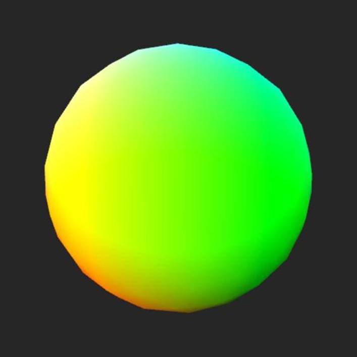
You can find this example in the file 03-lighting-vertex.html. It produces the result shown in Figure 11-3.
Adding per-pixel lighting
As you can see in Figure 11-3, it’s easy to make out the triangles in the band where the transition from light to shadow occurs. One solution to this problem is to move the calculations to the fragment shader. This is called per-fragment or per-pixel lighting because the light is calculating per pixel rather than per vertex. Doing calculations in the fragment shader can often produce better results but comes at the cost of using extra resources. Although the vertex shader needs only three calculations to cover a triangle, the fragment shader must calculate for every pixel drawn on the screen.
Figure 11-3: The sphere with per-vertex lighting
Diffuse light
The fragment needs to be able to access the vertex normal. Listing 11.21 shows the revised vertex shader with the calculations removed and the normal exported to a varying variable.
Listing 11.21 Vertex-shader for Per-pixel Lighting
attribute vec3 aVertex;
attribute vec3 aNormal;
uniform mat4 uModelView;
uniform mat4 uProjection;
uniform mat3 uNormalMatrix;
varying vec4 vPosition;
varying vec3 vNormal;
varying vec3 vColor;
void main(void) {
vPosition = uModelView * vec4(aVertex, 1.0);
vColor = aVertex.xyz * 0.5 + 0.5;
vNormal = uNormalMatrix * aNormal;
gl_Position = uProjection * vPosition;
}
The calculations in the fragment shader, shown in Listing 11.22, are almost identical to those from the vertex shader in Listing 11.19 and shouldn’t need further explanation.
Listing 11.22 Diffuse Light in the Fragment Shader
#ifdef GL_ES
precision mediump float;
#endif
uniform vec3 uLightPosition;
uniform float uAmbient;
varying vec4 vPosition;
varying vec3 vNormal;
varying vec3 vColor;
void main(void) {
vec3 normal = normalize(vNormal);
vec3 lightDir = normalize(uLightPosition - vPosition.xyz);
float diffuse = max(dot(normal, lightDir), 0.0);
vec3 color = vColor * (uAmbient + diffuse);
gl_FragColor = vec4(color, 1.0);
}
Now that we’ve moved to the fragment shader, we can also add the specular component to get a shiny highlight.
Specular light
To calculate the intense specular light component, you need two new vectors: the view direction and reflection direction. The view direction is a vector pointing from the view position to the point on the surface. If vPosition is the position relative to the eye, the direction is just -vPosition, normalized to unit length:
vec3 viewDir = normalize(-vPosition.xyz);
The reflection direction is the direction the light reflects off the surface. If you know the surface normal and direction of the incoming light, GLSL provides a reflect() function that calculates the reflected vector:
vec3 reflectDir = reflect(-lightDir, normal);
The amount of specular light that needs to be added to the surface point depends on the angle between these two vectors. As with the diffuse light, you can use the dot product of the vectors as a specular light value:
float specular = max(dot(reflectDir, viewDir), 0.0);
You can control the shininess of the surface by raising the specular value to some power:
specular = pow(specular, 20.0);
Finally, add the specular component to the lighting sum. Listing 11.23 shows the additions to the fragment shader.
Listing 11.23 Specular Light in the Fragment Shader
...
void main(void) {
...
vec3 viewDir = normalize(-vPosition.xyz);
vec3 reflectDir = reflect(-lightDir, normal);
float specular = max(dot(reflectDir, viewDir), 0.0);
specular = pow(specular, 20.0);
vec3 color = vColor * (uAmbient + diffuse + specular);
gl_FragColor = vec4(color, 1.0);
}
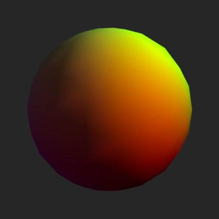
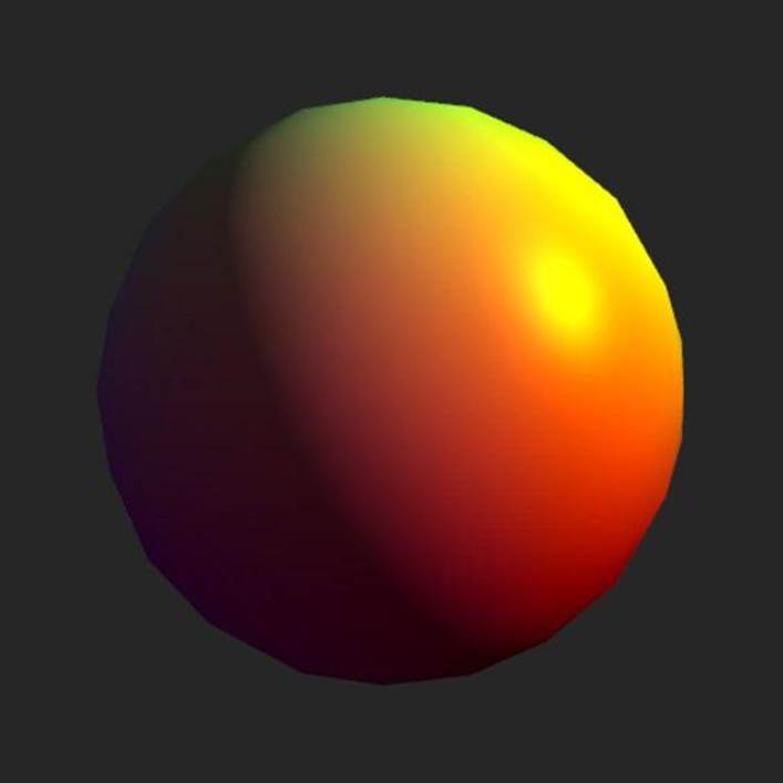
The result is shown in Figure 11-4. Moving the light calculations to the fragment shader gives a much smoother transition between the different shades, and the addition of a specular component adds a nice, shiny look to the surface. The code for this example is located in the file 04-lighting-fragment.html.
Figure 11-4: The sphere with per-pixel lighting
Creating textures
It’s time to get rid of that boring color gradient on the sphere and slap on something a bit more interesting. To use a texture image, start by creating a texture object:
var texture = gl.createTexture();
The texture object needs to be bound to a target to let WebGL know how you want to use it. The target you want is gl.TEXTURE_2D:
gl.bindTexture(gl.TEXTURE_2D, texture);
The functions gl.texParameteri() and gl.texParameterf() enable you to set parameters that control how the texture is used. For example, you can specify how WebGL should scale the texture image when it is viewed at different distances. The parameters gl.TEXTURE_MIN_FILTER andgl.TEXTURE_MAG_FILTER specify the scaling method used for minification and magnification, respectively:
gl.texParameteri(
gl.TEXTURE_2D, gl.TEXTURE_MIN_FILTER, gl.LINEAR
);
gl.texParameteri(
gl.TEXTURE_2D, gl.TEXTURE_MAG_FILTER, gl.LINEAR
);
The value gl.NEAREST toggles the fast nearest-neighbor method, whereas gl.LINEAR chooses the smoother linear filter.
A term you’ll probably encounter now and then is mipmaps. Mipmaps are precalculated, downscaled versions of the texture image you can use to increase performance. You can make WebGL generate the mipmaps automatically by calling the gl.generateMipmaps() function:
gl.generateMipmaps(gl.TEXTURE_2D);
You can then set the minification parameter to one of the values:
• gl.NEAREST_MIPMAP_NEAREST
• gl.LINEAR_MIPMAP_NEAREST
• gl.NEAREST_MIPMAP_LINEAR
• gl.LINEAR_MIPMAP_LINEAR
![]()
If you do use mipmapping, the dimensions of your textures must be powers of two, such as 512x512, 256x256, or 2048x1024. The mipmap images are entered into mipmap levels where each level contains a version that scales to 1/2n, where n is the level number.
dLoading image data
You’re now ready to load some pixels into the texture object. You do this with the texImage2D() function:
gl.texImage2D(
gl.TEXTURE_2D, 0, gl.RGBA, gl.RGBA, gl.UNSIGNED_BYTE, image
);
The second parameter specifies the mipmap level into which this data should be loaded. Because you’re not using mipmaps here, the data should be loaded into level 0. The third parameter is the pixel format used internally by the texture, and the fourth parameter is the pixel format used in the image data. It’s not actually possible to convert between formats when loading data, so the two arguments must match. Valid formats are gl.RGBA, gl.RGB, gl.ALPHA, gl.LUMINANCE, and gl.LUMINANCE_ALPHA. The fifth parameter specifies the data type of the pixel values, usuallygl.UNSIGNED_BYTE. Consult Appendix B or the WebGL specification for detailed information on pixel formats and types. The last parameter, image, is the source of the image data and can be an img element, a canvas element, or a video element.
You can also use gl.texImage2D() to load pixel values from an array. In that case, the function uses a few additional parameters that specify the dimensions of the texture data:
// create array that can hold a 200x100 px RGBA image
var image = new Uint8Array(200 * 100 * 4);
// fill array with values
...
// and load the data into the texture
gl.texImage2D(
gl.TEXTURE_2D, 0, gl.RGBA,
200, 100, 0, // width, height, border
gl.RGBA, gl.UNSIGNED_BYTE, image
);
The type of the array passed to gl.texImage2D() must match the data type specified in the call. For example, gl.UNSIGNED_BYTE requires a Uint8Array. Listing 11.24 shows the texture creation combined in a function for the helper module.
Listing 11.24 Creating Texture Objects
jewel.webgl = (function() {
...
function createTextureObject(gl, image) {
var texture = gl.createTexture();
gl.bindTexture(gl.TEXTURE_2D, texture);
gl.texParameteri(
gl.TEXTURE_2D, gl.TEXTURE_MIN_FILTER, gl.LINEAR);
gl.texParameteri(
gl.TEXTURE_2D, gl.TEXTURE_MAG_FILTER, gl.LINEAR);
gl.texImage2D(gl.TEXTURE_2D, 0,
gl.RGBA, gl.RGBA, gl.UNSIGNED_BYTE, image);
gl.bindTexture(gl.TEXTURE_2D, null);
return texture;
}
...
})();
When you are loading data from an img element, the image must be fully loaded before calling gl.texImage2D(). Just wait until the load event fires on the img element before you create the texture:
var image = new Image();
image.addEventListener(“load”, function() {
// create and load texture data...
}, false);
image.src = “earthmap.jpg”;
You can also add a listener to the error event on the img element if you want to catch loading errors.
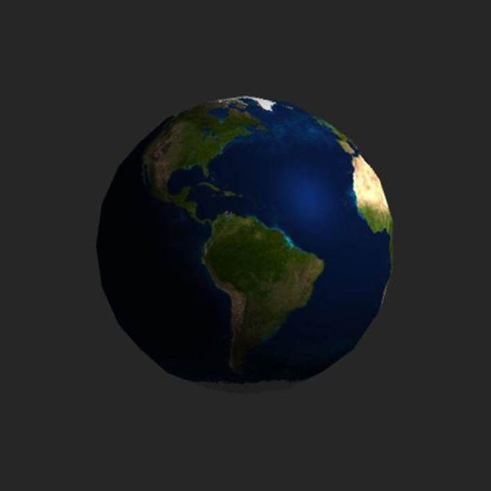
In the code archive for this chapter, I included the texture of the Earth’s surface, downloaded from NASA’s web site: http://visibleearth.nasa.gov/view_rec.php?vev1id=11612. Figure 11-5 shows the texture map. In the following example, I show you how to apply this texture map to the sphere to make a rotating planet.
Using textures in shaders
Textures are referenced in the fragment shader using a uniform variable with a special data type. The sampler2D type is a handle that points to the texture data and can be used with a function called texture2D() to sample color values from the texture image.
uniform sampler2D uTexture;
gl_FragColor = texture2D(uTexture, vTexCoord);
Figure 11-5: Earth texture map

The second parameter to texture2D() is a vec2 with x and y values between 0 and 1, specifying the point on the texture image that should be sampled. The upper-left corner is given as (0.0, 0.0) and the lower right as (1.0, 1.0). Texture coordinates are often created as buffers and accessed in the vertex shader alongside the vertices. You can use a varying variable to transfer and interpolate the coordinates to the fragment shader to create continuous texture mapping across the surface of the triangle. For example, to map an image to a flat rectangle, you would specify the texture coordinates (0.0, 0.0) at the upper-left vertex, (1.0, 0.0) at the upper-right vertex, and so on.
Calculating texture coordinates
For intricate 3D objects, the modeler or texture artist often assigns texture coordinates in the modeling application and then exports them with the rest of the model data. Almost all model formats, including Collada, are able to attach texture coordinates to the vertices. However, because we’re dealing with a simple sphere in this example, I instead show how you can calculate these coordinates manually in the shader.
We do the calculations in the fragment shader, but first we need a bit of information from the vertex shader. The texture coordinates on the sphere depend on the position of the given point. For the purpose of calculating spherical coordinates, the surface normal is just as good, so the vertex shader should export the normal to a varying vector. The normal must be the unmodified, pre-transformation normal. Listing 11.25 shows the new varying variable in the vertex shader.
Listing 11.25 Passing the Normal to the Fragment Shader
...
varying vec3 vOrgNormal;
void main(void) {
...
vOrgNormal = aNormal;
}
The fragment shader calculates the spherical coordinates from the normal and uses those as texture coordinates. In a spherical coordinate system, a point is described by a radial distance and two angles, usually denoted by the Greek letters θ (theta) and ϕ (phi). The relation between Cartesian (x,y,z) and spherical coordinates is as follows:
radius = sqrt(x*x + y*y + z*z)
theta = acos(y / radius)
phi = atan(z / x)
All points on the surface of a sphere are at the same distance from the center, so only the two angles are important. Because we used the normal rather than the vertex position, we know the radius is equal to 1, so the conversion simplifies to
theta = acos(y)
phi = atan(z / x)
If you apply these equations to the normal vector in the fragment shader, you can use theta and phi as texture coordinates, as shown in Listing 11.26.
Listing 11.26 Fragment Shader with Spherical Texture
...
varying vec3 vOrgNormal;
uniform sampler2D uTexture;
void main(void) {
...
float theta = acos(vOrgNormal.y);
float phi = atan(vOrgNormal.z, vOrgNormal.x);
vec2 texCoord = vec2(-phi / 2.0, theta) / 3.14159;
vec4 texColor = texture2D(uTexture, texCoord);
vec3 color = texColor.rgb * (uAmbient + diffuse + specular);
gl_FragColor = vec4(color, 1.0);
}
Texture coordinates range from 0 to 1, but the theta and phi angles are given in radians. The theta angle goes from zero to pi and phi goes from zero to 2 pi. To account for this, both coordinates are divided by pi and phi is further divided by 2. The pixel value is then fetched from the texture image using the texture2D() function and the newly calculated texture coordinates. The file 05-texture.html contains the full sample code for rendering the textured sphere shown in Figure 11-6.
Figure 11-6: Sphere with planet texture
This concludes the walkthrough of the WebGL API and you should now have a basic understanding of how you can use WebGL to create 3D graphics for your games and applications. The next section shows you how to use WebGL to add a new display module to Jewel Warrior.
Creating the WebGL display
You now know the basics of WebGL, so it’s time to get to work. The new display module, shown in Listing 11.27, goes in the file display.webgl.js. It should expose the same functions as the canvas display module so the two can be used interchangeably.
Listing 11.27 The WebGL Display Module
jewel.display = (function() {
var animations = [],
previousCycle,
firstRun = true,
jewels;
function initialize(callback) {
if (firstRun) {
setup();
firstRun = false;
}
requestAnimationFrame(cycle);
callback();
}
function setup() {
}
function setCursor() { }
function levelUp() { }
function gameOver() { }
function redraw() { }
function moveJewels() { }
function removeJewels() { }
return {
initialize : initialize,
redraw : redraw,
setCursor : setCursor,
moveJewels : moveJewels,
removeJewels : removeJewels,
refill : redraw,
levelUp : levelUp,
gameOver : gameOver
};
})();
The WebGL display module can borrow the addAnimation() and renderAnimations() functions from the canvas module, so they can be copied from display.canvas.js without any changes.
Loading the WebGL files
The addition of an extra display module complicates the load order a bit. The WebGL display should be first priority with canvas in second place and the DOM display as a final resort. Listing 11.28 shows the modifications to the second stage of the loader.js script. Note that Modernizr’s WebGL detection can report false positives on some iOS devices. The custom test in Listing 11.28 returns true only if it is actually possibly to create a WebGL context.
Listing 11.28 Loading the WebGL Display Module
Modernizr.addTest(“webgl2”, function() {
try {
var canvas = document.createElement(“canvas”),
ctx = canvas.getContext(“experimental-webgl”);
return !!ctx;
} catch(e) {
return false;
};
});
...
// loading stage 2
if (Modernizr.standalone) {
Modernizr.load([{
test : Modernizr.webgl2,
yep : [
“loader!scripts/webgl.js”,
“loader!scripts/webgl-debug.js”,
“loader!scripts/glMatrix-0.9.5.min.js”,
“loader!scripts/display.webgl.js”,
“loader!images/jewelpattern.jpg”,
]
},{
test : Modernizr.canvas && !Modernizr.webgl2,
yep : “loader!scripts/display.canvas.js”
},{
test : !Modernizr.canvas,
yep : “loader!scripts/display.dom.js”
},{
...
}]);
}
Modernizr’s script loader doesn’t support nested tests, so you need three independent tests to handle the three load cases. The first test loads the WebGL display if WebGL is supported. The second test loads the canvas display if canvas is supported but WebGL is not. The third test loads the DOM display only if canvas — and by extension WebGL — is unavailable.
Setting up WebGL
The first step to setting up the WebGL display is adding a new canvas element and getting a WebGL context object for the canvas. You do this by using the setup() function, as shown in Listing 11.29.
Listing 11.29 Setting Up the WebGL Display
jewel.display = (function() {
var dom = jewel.dom,
webgl = jewel.webgl,
$ = dom.$,
canvas, gl,
cursor,
cols, rows,
...
function setup() {
var boardElement = $(”#game-screen .game-board”)[0];
cols = jewel.settings.cols;
rows = jewel.settings.rows;
jewels = [];
canvas = document.createElement(”canvas”);
gl = canvas.getContext(”experimental-webgl”);
dom.addClass(canvas, ”board”);
canvas.width = cols * jewel.settings.jewelSize;
canvas.height = rows * jewel.settings.jewelSize;
boardElement.appendChild(canvas);
setupGL();
}
function setCursor(x, y, selected) {
cursor = null;
if (arguments.length > 0) {
cursor = {
x : x,
y : y,
selected : selected
};
}
}
...
})();
The setup() function ends by calling a setupGL() function. This function, shown in Listing 11.30, is responsible for setting up the WebGL context so it’s ready to render the game display.
Listing 11.30 Initializing the WebGL Context
jewel.display = (function() {
var program,
geometry,
aVertex, aNormal,
uScale, uColor,
...
function setupGL() {
gl.enable(gl.DEPTH_TEST);
gl.enable(gl.CULL_FACE);
gl.enable(gl.BLEND);
gl.blendFunc(gl.SRC_ALPHA, gl.ONE);
program = setupShaders();
setupTexture();
gl.useProgram(program);
aVertex = gl.getAttribLocation(program, “aVertex”);
aNormal = gl.getAttribLocation(program, “aNormal”);
uScale = gl.getUniformLocation(program, “uScale”);
uColor = gl.getUniformLocation(program, “uColor”);
gl.enableVertexAttribArray(aVertex);
gl.enableVertexAttribArray(aNormal);
gl.uniform1f(
gl.getUniformLocation(program, “uAmbient”),
0.12
);
gl.uniform3f(
gl.getUniformLocation(program, “uLightPosition”),
20, 15, -10
);
webgl.loadModel(gl, “models/jewel.dae”, function(geom) {
geometry = geom;
});
webgl.setProjection(
gl, program, 60, cols/rows, 0.1, 100
);
}
...
})();
Note that a few of the uniform locations as well as the attribute locations are stored for later use. The reason for storing them is to avoid having to look them up in each render cycle. The locations don’t change, so you don’t need to query them more than once.
The jewels list in the WebGL display differs from that in the canvas display. Instead of the two-dimensional array structure, jewels is now just an array of jewel objects. The createJewel() function in Listing 11.31 adds new jewels to the list.
Listing 11.31 Creating New Jewels
jewel.display = (function() {
...
function createJewel(x, y, type) {
var jewel = {
x : x,
y : y,
type : type,
rnd : Math.random() * 2 - 1,
scale : 1
};
jewels.push(jewel);
return jewel;
}
function getJewel(x, y) {
return jewels.filter(function(j){
return j.x == x && j.y == y
})[0];
}
...
})();
The rnd property on the jewel object can be used to add variation to the jewels so they don’t all look exactly alike. The getJewel() function is a helper function that searches the list for jewels matching a given set of coordinates. Both of these functions are used in the redraw() function, as shown in Listing 11.32.
Listing 11.32 Redrawing the Board
jewel.display = (function() {
...
function redraw(newJewels, callback) {
var x, y,
jewel, type;
for (x = 0; x < cols; x++) {
for (y = 0; y < rows; y++) {
type = newJewels[x][y];
jewel = getJewel(x, y);
if (jewel) {
jewel.type = type;
} else {
createJewel(x, y, type);
}
}
}
callback();
}
...
})();
The redraw() function iterates over all positions on the board. If a jewel object exists in the given position, its type is switched; otherwise, a new jewel object is created.
Rendering jewels
Figure 11-7 shows the jewel model that the WebGL display uses. You can find this isolated jewel renderer in the file 06-jewel.html.
Blending and transparency
In the setup() function, notice that two new settings are enabled: gl.BLEND and gl.CULL_FACE. Both are used to give the jewels a semitransparent appearance.
Enabling gl.BLEND lets you set rules for how the color output from the fragment shader is blended with the color value underneath the fragment. You set the blending rule with the gl.blendFunc() function. This function takes two parameters, a source factor and destination factor, that describe how the two colors are computed. The destination is the existing color, and the source is the incoming color drawn on top. Setting the source factor to gl.SRC_ALPHA means that the RGB values in the fragment color are multiplied by the alpha value; setting the destination factor togl.ONE means that the existing color is just multiplied by 1. You can find the full list of blends in Appendix C, which is part of the online bonus content on the book’s companion website.
Figure 11-7: The jewel model
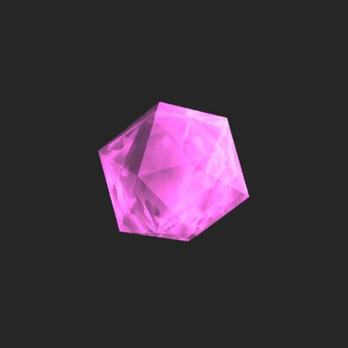
The gl.CULL_FACE setting enables face culling, which essentially removes the triangles facing away from the viewpoint. The direction in which a triangle is facing depends on whether it’s drawn clockwise or counterclockwise on the screen. The default mode is that triangles that are drawn counterclockwise face the viewer, whereas clockwise triangles face away. When culling is enabled, you can switch between culling front-facing and back-facing triangles with the gl.cullFace() function. This function takes a single argument, which is either gl.FRONT or gl.BACK. If you cull the front-facing triangles, only the internal surface of the object is visible. If you then do another render on top of that with blending enabled and back-facing triangles culled, the effect is a translucent object where the backside is visible through the model.
Drawing jewels
The render cycle is similar to the cycle from the canvas display, but it calls only the draw() function after the model file finishes loading. Listing 11.33 shows the cycle() function.
Listing 11.33 The Render Cycle
jewel.display = (function() {
...
function cycle(time) {
renderAnimations(time, previousCycle);
if (geometry) {
draw();
}
previousCycle = time;
requestAnimationFrame(cycle);
}
...
})();
Despite its name, the draw() function doesn’t actually do any drawing. Its task is to clear the canvas and bind the buffers. Listing 11.34 shows the function.
Listing 11.34 Preparing for the Next Frame
jewel.display = (function() {
...
function draw() {
gl.clear(gl.COLOR_BUFFER_BIT | gl.DEPTH_BUFFER_BIT);
gl.viewport(0, 0, canvas.width, canvas.height);
gl.bindBuffer(gl.ARRAY_BUFFER, geometry.vbo);
gl.vertexAttribPointer(
aVertex, 3, gl.FLOAT, false, 0, 0);
gl.bindBuffer(gl.ARRAY_BUFFER, geometry.nbo);
gl.vertexAttribPointer(
aNormal, 3, gl.FLOAT, false, 0, 0);
gl.bindBuffer(gl.ELEMENT_ARRAY_BUFFER, geometry.ibo);
jewels.forEach(drawJewel);
}
...
})();
All the jewels use the same geometry, so you need to bind the buffers only once. You can then draw the model as many times as you want. The draw() function finishes by calling drawJewel() on all jewels. This function is shown in Listing 11.35.
Listing 11.35 Drawing a Single Jewel
jewel.display = (function() {
...
var colors = [
[0.1, 0.8, 0.1],
[0.9, 0.1, 0.1],
[0.9, 0.3, 0.8],
[0.8, 1.0, 1.0],
[0.2, 0.4, 1.0],
[1.0, 0.4, 0.1],
[1.0, 0.9, 0.1]
];
function drawJewel(jewel) {
var x = jewel.x - cols / 2 + 0.5, // make position
y = -jewel.y + rows / 2 - 0.5, // relative to center
scale = jewel.scale,
n = geometry.num;
var mv = webgl.setModelView(gl, program,
[x * 4.4, y * 4.4, -32], // scale and move back
Date.now() / 1500 + jewel.rnd * 100, // rotate
[0, 1, 0.1] // rotation axis
);
webgl.setNormalMatrix(gl, program, mv);
// add effect for selected jewel
if (cursor && jewel.x==cursor.x && jewel.y==cursor.y) {
scale *= 1.0 + Math.sin(Date.now() / 100) * 0.1
}
gl.uniform1f(uScale, scale);
gl.uniform3fv(uColor, colors[jewel.type]);
gl.cullFace(gl.FRONT);
gl.drawElements(gl.TRIANGLES, n, gl.UNSIGNED_SHORT, 0);
gl.cullFace(gl.BACK);
gl.drawElements(gl.TRIANGLES, n, gl.UNSIGNED_SHORT, 0);
}
...
})();
First, the model-view and normal matrices are updated to match the position of the current jewel. The jewel position is also scaled and moved back to get the full 8x8 grid of jewels to fit within the confines of the canvas. The rotation of the jewel is a function of the current time. Adding the jewel’s own rnd number to the rotation avoids having all the jewels rotating in sync.
If the jewel happens to be selected — that is, if its position matches that of the cursor — the jewel scale is multiplied by a sine function to create a throbbing effect. The uniform scale factor is applied in the vertex shader. By multiplying the vertex position from the aVertex attribute with theuScale variable, you can control the size of the rendered jewel:
vPosition = uModelView * vec4(aVertex * uScale, 1.0);
When the matrices and uniforms are updated, the drawing can commence. The rendering is split in two passes. The first pass renders the backside of the jewel, and the second pass renders the front of the jewel.
Creating the jewel surface
The shaders are created in the setupShaders() function and build off the ones you saw already in the lighting and texturing examples. The flat faces of the jewel don’t require the high-resolution per-pixel lighting, however, so the lighting is done per-vertex. This type of lighting also gives a better specular light in this particular scenario. The shader code is too big to include here but you can find the complete code for setupShaders() in the display.webgl.js file included in the code archive for this chapter. The fragment shader uses a mix of a solid color and texture, as shown in Figure 11-8, to color the jewel. The texture provides noise to the jewel, simulating a bit of structure in the jewel.
Figure 11-8: Noise texture for the jewels
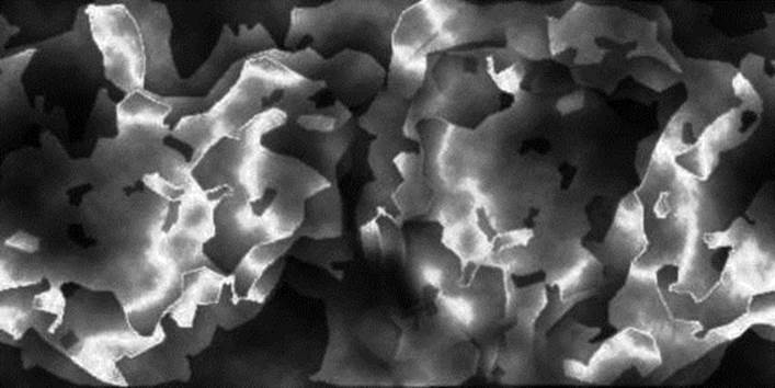
The texture is created in the setupTexture() function shown in Listing 11.36.
Listing 11.36 Setting up the Jewel Texture
jewel.display = (function() {
...
function setupTexture() {
var image = new Image();
image.addEventListener(“load”, function() {
var texture = webgl.createTextureObject(gl, image);
gl.uniform1i(
gl.getUniformLocation(program, “uTexture”),
“uTexture”, 0
);
gl.activeTexture(gl.TEXTURE0);
gl.bindTexture(gl.TEXTURE_2D, texture);
}, false);
image.src = “images/jewelpattern.jpg”;
}
...
})();
The solid color that is mixed with the jewel texture comes from the uniform variable set by the drawJewel() function:
uniform vec3 uColor;
The shader fetches a sample from the texture image using the spherical coordinates you saw earlier. It’s the brightness of the texture that is important, and because the texture is grayscale, you need only one of the RGB channels:
float texColor = texture2D(uTexture, texCoord).r;
The texture color acts as an extra light component and just adds to the sum of lights:
float light = uAmbient + vDiffuse + vSpecular + texColor;
Finally, the lighting is applied to the jewel color, and the result is assigned to the fragment:
gl_FragColor = vec4(uColor * light, 0.7);
The 0.7 alpha value in the fragment color makes the color semitransparent so the backside of the jewel shines through. Figure 11-9 shows the game board as rendered with the WebGL display.
Figure 11-9: The WebGL jewel board
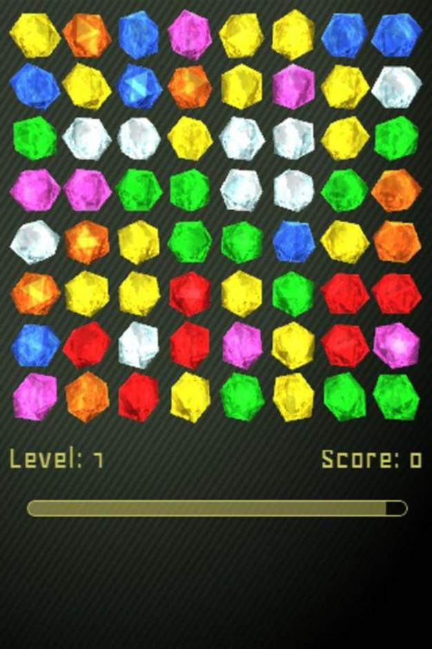
Animating the jewels
The last step is to implement the animations for the various game actions.
Moving and swapping jewels
The moveJewels() function, shown in Listing 11.37, is similar to its canvas counterpart. It adds a new animation for each moving jewel, moving the jewel toward its destination in the render() function.
Listing 11.37 Moving Jewels
jewel.display = (function() {
...
function moveJewels(movedJewels, callback) {
var n = movedJewels.length;
movedJewels.forEach(function(mover) {
var jewel = getJewel(mover.fromX, mover.fromY),
dx = mover.toX - mover.fromX,
dy = mover.toY - mover.fromY,
dist = Math.abs(dx) + Math.abs(dy);
if (!jewel) { // new jewel entering from the top
jewel = createJewel(mover.fromX, mover.fromY,
mover.type);
}
addAnimation(200 * dist, {
render : function(pos) {
pos = Math.sin(pos * Math.PI / 2);
jewel.x = mover.fromX + dx * pos;
jewel.y = mover.fromY + dy * pos;
},
done : function() {
jewel.x = mover.toX;
jewel.y = mover.toY;
if (--n === 0) { // last one calls callback
callback();
}
}
});
});
}
...
})();
When you are iterating over the list of moving jewels, the relevant jewel object is fetched from the jewels list using the getJewel() function. The getJewel() function returns undefined if the search fails; in that case, a new jewel is created. This handles the case where new jewels move in from the top of the screen.
Removing matched jewels
In the canvas display module, removing jewels causes a spinning and shrinking effect on the jewels. The removeJewels() function in Listing 11.38 adds a variation of that to the WebGL display.
Listing 11.38 Removing Jewels
jewel.display = (function() {
...
function removeJewels(removedJewels, callback) {
var n = removedJewels.length;
removedJewels.forEach(function(removed) {
var jewel = getJewel(removed.x, removed.y),
y = jewel.y, // original coordinates
x = jewel.x;
addAnimation(400, {
render : function(pos) {
jewel.x = x + jewel.rnd * pos * 2;
jewel.y = y + pos * pos * 2;
jewel.scale = 1 - pos;
},
done : function() {
jewels.splice(jewels.indexOf(jewel), 1);
if (--n == 0) { // last one calls callback
callback();
}
}
});
});
}
...
})();
The animation added by the removeJewels() function makes the jewel fall toward the bottom while shrinking. The pos value goes from 0 to 1 over the course of the animation, so subtracting it from the jewel scale causes the jewel to shrink until it disappears. The vertical movement uses thepos factor squared to simulate downward acceleration due to gravity:
jewel.y = y + pos * pos * 2;
In addition to the vertical movement, using the random rnd value adds a bit of horizontal movement so it doesn’t fall straight down:
jewel.x = x + jewel.rnd * pos * 2;
You can increase or decrease the two factors, currently set to 2, to speed up the movement in either of the directions.
When the animation ends and the done() function is called, the jewel is removed from the jewels list using the splice() array method.
Leveling up and ending the game
Three functions remain: refill(), gameOver(), and levelUp(). There are endless possibilities for what the refill animation could look like. I leave that one up to you as an exercise. The current implementation simply redirects the call to the redraw() function:
function refill(newJewels, callback) {
redraw(newJewels, callback);
}
This function works fine but is, of course, not very exciting.
The animation from the removeJewels()function can be reused to implement the gameOver() function, as shown in Listing 11.39. Just call removeJewels() on the entire list of jewels to make the whole board fall apart.
Listing 11.39 Removing All Jewels
jewel.display = (function() {
...
function gameOver(callback) {
removeJewels(jewels, callback);
}
...
})();
That leaves the levelUp() function. Let’s add a highlight effect to all the jewels by increasing the ambient light component. This causes all jewels to briefly light up. Listing 11.40 shows the animation.
Listing 11.40 The Level Up Animation
jewel.display = (function() {
...
function levelUp(callback) {
addAnimation(500, {
render : function(pos) {
gl.uniform1f(
gl.getUniformLocation(program, “uAmbient”),
0.12 + Math.sin(pos * Math.PI) * 0.5
);
},
done : callback
});
}
...
})();
That’s the last of the WebGL display module. You now have three different options for displaying the game graphics.
Summary
You are now equipped to start using WebGL in your applications and games. This chapter introduced you to the basics of the WebGL API; the GLSL language used in shaders; and a few techniques you can use to add textures, lighting, and blending effects to your rendered objects. It also showed how to use WebGL to create a more advanced display module for the Jewel Warrior game.
Although WebGL is still immature, every day brings news of fresh experiments and projects. Several 3D engines based on WebGL have already emerged, simplifying the task of building complex 3D applications. Perhaps the greatest roadblock at the moment is the question of Internet Explorer. With no support for WebGL in sight, a large number of users won’t be able to experience WebGL content. That said, alternative solutions, including third-party plugins, are in the works. I hope the future will allow everyone to take part in these great advances in web graphics.
All materials on the site are licensed Creative Commons Attribution-Sharealike 3.0 Unported CC BY-SA 3.0 & GNU Free Documentation License (GFDL)
If you are the copyright holder of any material contained on our site and intend to remove it, please contact our site administrator for approval.
© 2016-2026 All site design rights belong to S.Y.A.