Java: Artificial Intelligence; Made Easy, w/ Java Programming; Learn to Create your * Problem Solving * Algorithms! TODAY! w/ Machine Learning & Data Structures, 1st Edition (2015)
Chapter 3. Search Strategies
==== ==== ==== ==== ====
As mentioned earlier, the way the search algorithm picks a path from the frontier will determine the overall algorithm search strategy.
Now that we’ve developed our search algorithm, we can now modify it to suit any situation that arises.
Below are the four main ways that the search algorithm will pick a path to explore. The path picked from the frontier is either:
- the most recently added (Stack)
- the least recently added (Queue)
- the one with the least cost (Priority Queue)
- the one with the most value (Priority Queue)
We’ll explore and analyze each strategy and implement them with our search algorithm.
Chapter 3.1: Depth-First Search
==== ==== ==== ==== ====
In Depth-First Search, the algorithm treats the Frontier Options as a Stack. Therefore, if the algorithm has a list of unexplored options it has yet to examine, it will explore the options and sub-options first.
Use Depth-First Search When:
1. You expect long path lengths; in other words, the solutions will have long sets of options to get there
1. You don’t expect any nodes that are subnodes to each other)
1. You don’t have much space available
Don’t use Depth-First Search When:
• The three looks fairly shallow. In other words, there aren’t many levels of Option nodes in the tree
• If having the best possible solution is very important
Example: The Depth-First Search Algorithm
Consider the graph below. If all these nodes are placed on a to-do list for the algorithm, the last node added to the frontier would be processed first.
Node #1’s options are added to the frontier: #2, #7, and #8. If Node #2 was added last, it would be processed first. So Nodes #3 and #6 would be added. If #3 was added last, then it would be processed first - so that means adding #4 and #5 to the frontier. The node depths are explored first - hence, why it’s called DEPTH-FIRST search.
Algorithm Analysis: Depth-First Search
Is it Complete?
Sort of. Why? If there are any loops or cycles in the graph (meaning one of the end nodes link up to the beginning nodes, thus creating a loop) the algorithm might be stuck. It will keep exploring the end node, the beginning node, the path between them, the end node again, and so on and so on - probably in a sort of infinite loop.
On the other hand, if there are no loops or cycles in the node network, this algorithm is complete.
Is it Optimal?
No. If it gives off the first solution it encounters, it may not necessarily be the best one. There may be better solutions that have yet to be encountered before the algorithm gets to it.
What is its Time Complexity?
O(b^m)
Meaning, at the worst-case scenario, the algorithm will explore every node and reach the furthest tree depth. For example, if a node in a tree has up to 2 options and the entire tree can be up to 4 levels deep, the worst-case complexity will be 2x2x2x2 = 16 nodes possibly explored.
What is its Space Complexity?
O(b*m)
Meaning, at the worst-case scenario, a path for unexplored nodes will be stored in memory for every node explored.
The longest path possible is the furthest tree depth. Also, every node has a maximum amount of nodes it can explore.
For example, if a tree will have up to 2 options per node and the tree can be 4 levels deep, then the algorithm will store 2x4 = 8 units of memory
Chapter 3.2: Breadth-First Search
==== ==== ==== ==== ====
While Depth-first search has a Stack for the frontier, Breadth-first search has a Queue. In other words, if the algorithm has a list of options to explore, it will select the earliest added options and sub-options.
Use Breadth-First Search When:
• you don’t have to worry about memory space
• you NEED a solution with the least amount of options chosen
• there are some options that can be explored that don’t need depth
Don’t use Breadth-First Search When:
• solutions tend to need a lot of options chosen (i.e. they’re deep into the tree)
• you have a limited amount of space
• There’s a high branching factor (nodes with many subnodes/options)
Example: The Breadth-First Search Algorithm
Consider the graph below. If all these nodes are placed on a to-do list for the algorithm, Node #1 would be processed first, then it’s sub-nodes #8, #7, #2 would be added to the frontier in that order. Since Node #8 was entered first, it will be processed first. So Nodes #9 and #12 are added to the frontier. Then Node #7 is processed. Then Node #2, which adds Nodes #6 and #3 to the frontier. Then node #12 is processed, and so on. Overall, the algorithm will explore all nodes per level first - hence why it’s called BREADTH-FIRST search.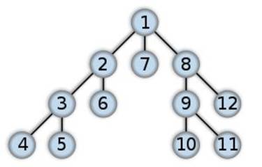
Algorithm Analysis: Breadth-First Search
Is it Complete?
Yes, as long as there’s a limited number of subnodes. When there are nodes that are children to each other (for example: Node X is a sub-node to Node Y, and vice-versa), this would normally create a loop for Depth-first search. Node X would be added to the frontier, processed, then Node Y would be added and processed, then Node X is added, and so on - in an infinite loop. This won’t happen in BFS. If Node X was added, all other nodes in the frontier would have been processed first.
However, if a tree has infinite subnodes per node, then BFS certainly won’t stop. There will be just too many nodes to explore.
Hence, as long as there’s a finite number of subnodes per node, you can guarantee that BFS will not loop indefinitely.
Is it Optimal?
Possibly. Because BFS is likely to find the solutions with the least number of options/steps, there is a chance the solution will be optimal.
What is its Time Complexity?
O(b^m)
Just like DFS, BFS will, at the worst-case scenario, explore every node and reach the furthest tree depth. For example, if a node in a tree has up to 3 options and the entire tree can be up to 4 levels deep, the worst-case complexity will be 3x3x3x3 = 81 nodes possibly explored.
What is its Space Complexity?
O(b^m)
At the worst-case scenario, BFS will explore every single node in the tree.
For example, if a tree will have up to 4 options per node and the tree can be 4 levels deep, then the algorithm will store 4^4 = 256 units of memory if it explores every node in that tree.
JAVA 03: Frontier Search as DFS and BFS
For the procedure below, select an IDE of your choice. You may also use online IDE’s such as rextester.com, ideone.com, or codepad.org.
========================= ======
When implementing Frontier Search, the algorithm will actually, by default, either be Depth-First Search or Breadth-First Search. This will depend on one key factor, as we will demonstrate below.
First, let’s recall the path picker from earlier:
/*
// HELPER FUNCTION #1:
// INPUT: a List of Paths
// OUTPUT: a Single Path
// EFFECT: based on positioning of your choice:
// - Select & remove a path
// - return that path
// NOTE: you can modify the position assignment to change the Search Strategy
*/
private Path pickPath(ArrayList<Path> f) {
int position = 0;
Path ret = f.get(position);
f.remove(position);
return ret;
}
Note how the path picker works. The output path, chosen from the input array (the frontier), is based on an index position. That index is set on the first line of the procedure:
int position = 0;
When items are entered into an array, they are sent to the end of the array like so:
[0: a][1: b][2: c] <- inserting [d]
[0: a][1: b][2: c][3: d]
So setting the position to 0 means that the front (earliest) path on the frontier is selected. In other words, the path picker will treat the frontier as a queue. Therefore it will be BFS.
int position = 0;
Before path picker call: [0: a][1: b][2: c][3: d]
After path picker call: [0: a][1: b][2: c] Selected For Processing: [d]
Otherwise, setting the position to the back (latest) path will need this line instead:
int position = f.size()-1;
The line above will set the position to the latest path added to the frontier. In other words, the path picker will treat the frontier as a stack. Therefore, it will be DFS.
int position = f.size()-1;
Before path picker call: [0: a][1: b][2: c][3: d]
After path picker call: [0: b][1: c][2: d] Selected For Processing: [a]
Now, let’s test everything we know so far on the below graph.
Bigger Search Graph: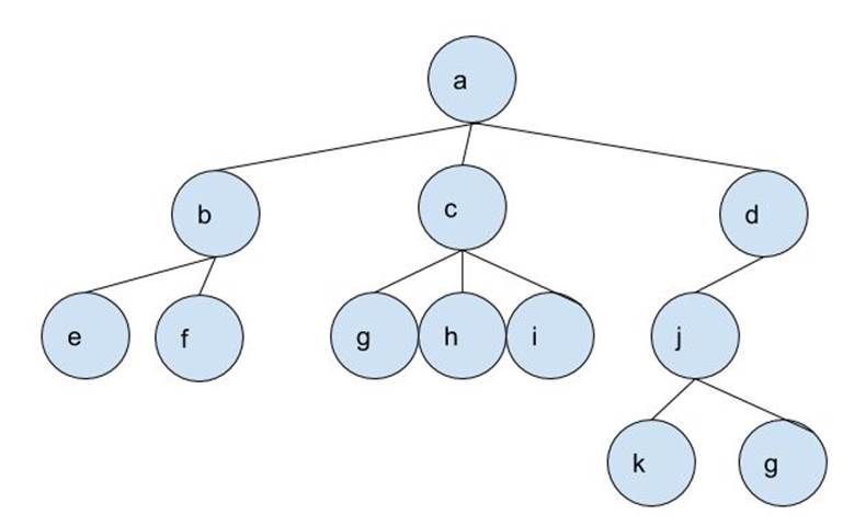
(The code for the graph above is found on ARCHIVE A02)
Place the code above into your Main() method to create the graph.
We start with the completed Node and Path classes from the previous chapter. If you need to copy the Search Algorithm, Nodes, and Paths, see ARCHIVE A01.
We will then modify the pickPath() method to be either DFS and BFS.
Step 1:
We’ll modify our pickPath() in the code below:
/*
// HELPER FUNCTION #1: (Modified)
*/
private Path pickPath(ArrayList<Path> f) {
int position;
// Breadth-First: uncomment line below to use
// position = 0;
// Depth-First: uncomment line below to use
// position = f.size()-1;
Path ret = f.get(position);
f.remove(position);
return ret;
}
Uncomment either of the lines above to set the position.
Step 2:
Next, we’ll run and test the algorithm.
Before we do this, make sure you have the printer() method in your Main() method. You can find this from either JAVA-02 or ARCHIVE A-01.
Moving on, simply add these two lines within your Main() method, just after the code for creating the search graph:
Path pg = a.search("g");
System.out.println(printer(pg));
There are two nodes that have “g” as their content. The algorithm will output either one as the solution depending on which search strategy you use.
If you set your pickPath() to DFS, the output lines should be:
Solution Found! Path: a, d, j, g,
Here’s what happened after the algorithm processed Node a:
- the algorithm added Nodes b, c, and d into the frontier
- Node d was added most recently; so it’ll be processed first
- Its subnode j is added
- Node j is added most recently; it’ll be processed first
- Nodes k and g2 are added
- Node g2 is added most recently; it’ll be processed first
- Node g2 is a goal. So a path with it and all its ancestor nodes is the solution path.
And if you look at the nodes carefully, you’ll notice that the algorithm went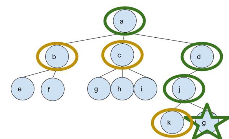 “Depth-First”:
Otherwise, if you set it to BFS, the output lines should be:
Solution Found! Path: a, c, g,
Here’s what happens after the algorithm processes Node a:
- the algorithm added Nodes b, c, and d into the frontier
- Node b is added first, so it’s processed first
- So Nodes e and f are added to the frontier
- Now the earliest node is c, so it’s then processed
- Nodes g1, h, and i are added
- Then Node d is processed, so Node j is added.
- Nodes e, f, and g1 are processed in that order, since they’re now the oldest nodes in the frontier
- Node g1 is a goal, so a path including it and its ancestors is the solution path.
And if you look at the nodes carefully, you’ll notice that the algorithm went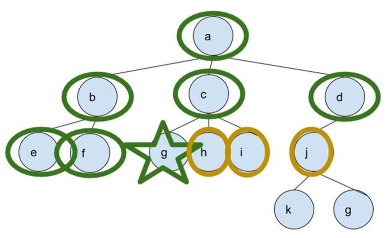 “Breadth-First”:
where the green-circled nodes have been processed already and the yellow-circled ones are in the frontier. They were supposed to be processed as well but the algorithm found a solution and finished instead.
Chapter 3.3: Lowest-Cost First Search
==== ==== ==== ==== ====
Sometimes, there can be costs between nodes and subnodes. For example, if a node had three subnodes, one of them would cost 10 to reach and the other two would cost 15.
So if the algorithm finds a solution, the path will have a total sum of all the costs required to reach the solution.
In this case, we want the solution that takes least overall cost to reach.
How it works:
The link between nodes and subnodes are called arcs. They can contain information vital for the algorithm to produce a viable, legal solution. For cost-based search algorithms, arcs will need costs between a node and a subnode.
[Node A] - - - -> arc A-B: cost=10 - - - ->[Node b]
Example: The Lowest-Cost-First Search Algorithm
Take note of the tree below. The red numbers indicate the cost to travel between nodes.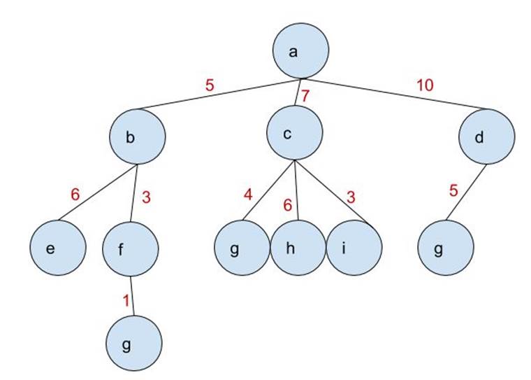
The algorithm will add Nodes B, C, and D to the frontier, as well as their respective costs, 5, 7, and 10. Which node will require the least cost to travel to? Node B. So Node B will be processed first, then Nodes E and F are added to the frontier, along with their respective total costs (Node E: 11 = 5+6, Node F: 8=3+5). Node C will be processed next, because it now has the lowest cost at 7. As you can see, the node that requires the least cost to reach is processed first.
Hence, why the algorithm is called LOWEST-COST FIRST.
Algorithm Analysis: Lowest-Cost-First Search
Is it Complete?
Yes, but there are certain conditions that need to be met. You can’t have arc costs be zero or any negative numbers. If this happens, you risk having the algorithm loop and run forever.
So as long as the arc costs have real, non-negative values, you can expect the algorithm to either deliver a solution or tell you that there isn’t any.
Is it Optimal?
Yes, and this is the algorithm variant’s main strength. You can guarantee that LCFS will give you a solution and a path that took the lowest cost to reach, as long as the arc costs are, again, real and non-negative values.
Otherwise, the path costs will be distorted and the solution produced might not be the optimal one.
What is its Time Complexity?
O(b^m)
At the worst-case, the LCFS algorithm will process all nodes in the tree. For example, if a tree had up to 5 subnodes per node and 4 levels down, you’re looking at 625 nodes to explore.
What is its Space Complexity?
O(b^m)
At the worst case, the LCFS algorithm will have every node in the tree stored into memory. So if you have a tree with 3 subnodes per node and 3 levels down, then you may have up to 27 nodes stored into memory.
Chapter 3.4: Heuristic Search
==== ==== ==== ==== ====
Another way to determine how to get the best path is to add heuristics to the arcs. The heuristic values can represent two things:
- A very low estimate of the total cost to reach a solution
- A value to maximize: the solution should have the highest value possible
In the first case, you can estimate the total cost to reach the nearest goal node from the start. It will be admissible as long as the cost isn’t overestimated.
In the second case, it will be the opposite of LCFS - each node-to-subnode arc will then have a value and the algorithm will find a solution with the highest value possible.
How it works:
The link between nodes and subnodes are called arcs. They can contain information vital for the algorithm to produce a viable, legal solution. For cost-based search algorithms, arcs will need costs between a node and a subnode.
[Node A] - - - -> arc A-B: cost=10 - - - ->[Node b] Example: Heuristic Search Algorithm
The tree below is the same one from LCFS, but now with added values to the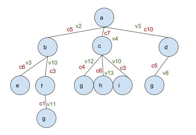 arcs.
arcs.
The Heuristic search algorithm will choose its nodes based on either the closest cost to the estimate or a maximum value. First, it adds Nodes b, c, and d to the frontier.
If, say, we estimate that the cost to get to Node g is 7, the algorithm will process Node c first because its cost is 7. So Nodes g, h, and i are added to the frontier, each with respective total costs 11 for g (4+7), 13 for h (6+7) and 10 for i (7+3). So Node b will then be processed next, because its cost (5) is currently closest to 7. Then its subnodes e (11 = 6+5) and f (8=5+3) are added. Node f is then processed, so a second Node g is added to the frontier, with a cost of (9=1+3+5). The recently added Node g has the closes cost to 7, so it’s then processed. It is a viable optimal solution, since the other g-nodes have costs of 11 and 15 respectively.
On the other hand, we can also have the algorithm pick a solution that creates the highest value. If we want to pick the path to Node g with the highest value, here’s what happens. Node c is processed first, because of its value (4). This adds Nodes g, h, and i with values 12, 13 and 10, respectively. Node h will then be processed next, but with no subnodes to add to the frontier. And once Node g is processed, i would be a viable solution, at a value of 12.
Algorithm Analysis: Heuristic Search
Is it Complete?
No, because there is a chance that the algorithm will be in an infinite loop once it cycles between two high-value nodes or two nodes closest to the estimate.
Is it Optimal?
Unfortunately no, but this is because the value-based or cost-based algorithms can be “greedy” at times. Meaning, the algorithm will only prefer the best possible node it has at the moment, but ignoring all other options. If deeper nodes have higher values, but the algorithm can’t get to them because it processes other nodes instead, then the algorithm might produce less optimal solutions instead.
What is its Time & Space Complexity?
O(b^m)
At the worst case, a heuristic search will explore every node in a tree and have each node stored in memory.
All materials on the site are licensed Creative Commons Attribution-Sharealike 3.0 Unported CC BY-SA 3.0 & GNU Free Documentation License (GFDL)
If you are the copyright holder of any material contained on our site and intend to remove it, please contact our site administrator for approval.
© 2016-2026 All site design rights belong to S.Y.A.