D3.js in Action (2015)

Part 1. D3.js fundamentals

The first three chapters introduce you to the fundamental aspects of D3 and get you started with creating graphical elements in SVG using data. Chapter 1 lays out how D3 relates to the DOM, HTML, CSS, and JavaScript, and provides a few examples of how to use D3 to create elements on a web page. Chapter 2 focuses on loading, measuring, processing, and changing your data in preparation for data visualization using the various functions D3 includes for data manipulation. Chapter 3 turns toward design and explains how you can use D3 color functions for more effective data visualization, as well as load external elements such as HTML for modal dialogs or icons in raster and vector formats. In all, part 1 shows you how to load, process, and visually represent data in SVG without relying on built-in layouts or components, which is critical for using and extending those layouts and components.

Chapter 1. An introduction to D3.js

This chapter covers

· The basics of HTML, CSS, and the Document Object Model (DOM)

· The principles of Scalable Vector Graphics (SVG)

· Data-binding and selections with D3

· Different data types and their data visualization methods

Note to print book readers: Many graphics in this book are meant to be viewed in color. The eBook versions display the color graphics, so they should be referred to as you read. To get your free eBook in PDF, ePub, and Kindle formats, go to manning.com/D3.jsinAction to register your print book.

D3 stands for data-driven documents. It’s a brand name, but also a class of applications that have been offered on the web in one form or another for years. For quite some time we’ve been building and working with data-driven documents such as interactive dashboards, rich internet applications, and dynamically driven content. In one sense, the D3.js library is an iterative step in a chain of technologies used for data-driven documents, but in another sense, it’s a radical step.

1.1. What is D3.js?

D3.js was created to fill a pressing need for web-accessible, sophisticated data visualization. Because of the library’s robust design, it does more than make charts. And that’s a good thing, because data visualization no longer refers to pie charts and line graphs. It now means maps and interactive diagrams and other tools and content integrated into news stories, data dashboards, reports, and everything else you see on the web.

D3.js’s creator, Mike Bostock, helped develop an earlier data visualization library, Protovis, and also developed Polymaps, a JavaScript library that provides vector- and tile-mapping capability in a lightweight form. These earlier endeavors would inform the creation of D3.js, which focuses on modern standards and modern browsers. As Bostock describes it, “This avoids proprietary representation and affords extraordinary flexibility, exposing the full capabilities of web standards such as CSS3, HTML5 and SVG” (http://d3js.org/). This is the radical nature of D3.js. Although it won’t run on Internet Explorer 6, the widespread adoption of standards on modern browsers has finally allowed web developers to deliver dynamic and interactive content seamlessly in the browser.

Until recently, you couldn’t build high-performance, rich internet applications in the browser unless you built them in Flash or as a Java applet. Flash and Java are still around on the internet, and especially for internal web apps, for this reason. D3.js provides the same performance, but integrated into web standards and the Document Object Model (DOM) at the core of HTML. D3 provides developers with the ability to create rich interactive and animated content based on data and tie that content to existing web page elements. It gives you the tools to create high-performance data dashboards and sophisticated data visualization, and to dynamically update traditional web content.

But D3 isn’t easy for people to pick up, because they often expect it to be a simple charting library. A case in point is the pie chart layout, which you’ll see in chapter 5. D3 doesn’t have one single function to create a pie chart. Rather, it has a function that processes your dataset with the necessary angles so that, if you pass the dataset to D3’s arc function, you get the drawing code necessary to represent those angles. And you need to use yet another function to create the paths necessary for that code. It’s a much longer process than using dedicated charting libraries, but the D3 process is also its strength. Although other charting libraries conveniently allow you to make line graphs and pie charts, they quickly break down when you want to make something more than that. Not D3, which allows you to build whatever data-driven graphics and interactivity you can imagine, and that’s why D3 is behind much of the most innovative and exciting information visualization on the web today.

1.2. How D3 works

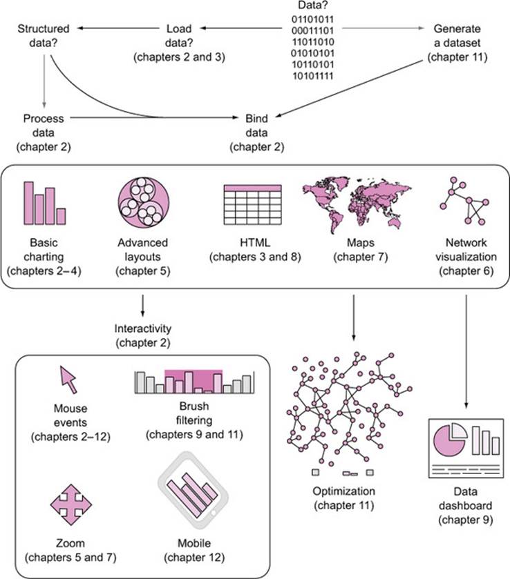
Let’s take a look at the principles of data visualization, as well as how D3 works in general. In figure 1.1 you see a rough map of how you might start with data and use D3 to process and represent that data, as well as add interactivity and optimize the data visualization you’ve created. In this chapter we’ll start by establishing the principles of how D3 selections and data-binding work and learning how D3 interacts with SVG and the DOM. Then we’ll look at data types that you’ll commonly encounter. Finally, we’ll use D3 to create simple DOM and SVG elements.

Figure 1.1. A map of how to approach data visualization with D3.js that highlights the approach in this book. Start at the top with data, and then follow the path depending on the type of data and the needs you’re addressing.

1.2.1. Data visualization is more than data visualization

You may think of data visualization as limited to pie charts, line charts, and the variety of charting methods popularized by Tufte and deployed in research. It’s much more than that. One of the core strengths of D3.js is that it allows for the creation of vector graphics for traditional charting, but also the creation of geospatial and network visualizations, as well as traditional HTML elements like tables, lists, and paragraphs. This broad-based approach to data visualization, where a map or a network graph or a table is just another kind of representation of data, is the core of the D3.js library’s appeal for application development.

Figures 1.2 through 1.8 show data visualization pieces that I’ve created with D3. They include maps and networks, along with more traditional pie charts and completely custom data visualization layouts based on the specific needs of my clients.

Figure 1.2. D3 can be used for simple charts, such as this set of multiple pie charts (explained in chapter 5) used to represent the differences in the use of language about nature in major US city planning (from the City Nature project at citynature.stanford.edu). Each pie shows the ratio of language referring to parks and open space (green) versus habitat (red) in city plans.

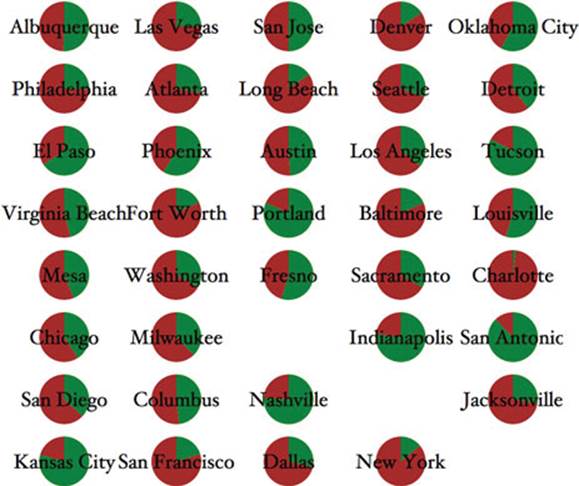
Figure 1.3. D3 can also be used to create web maps (see chapter 7), such as this map showing the ethnic makeup of major metropolitan areas in the United States.

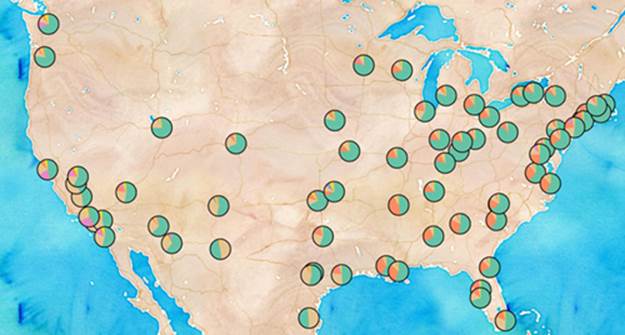
Figure 1.4. Maps in D3 aren’t limited to traditional Mercator web maps, and can be interactive globes, like this map of undersea communication cables, or other more unorthodox maps (see chapter 7).

Figure 1.5. D3 also provides robust capacities to create interactive network visualizations (see chapter 6). Here you see the social and coauthorship network of archaeologists working at the same dig for nearly 25 years.

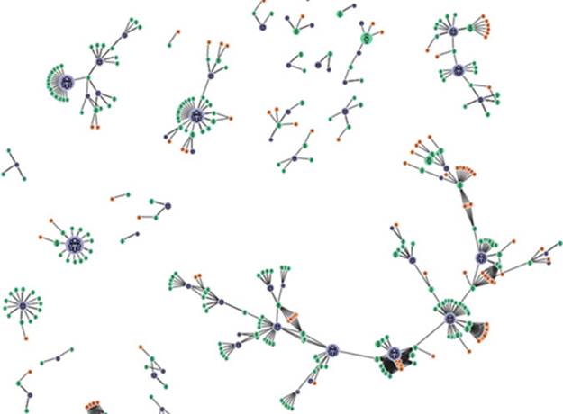
Figure 1.6. D3 includes a library of common data visualization layouts, such as the dendrogram (explained in chapter 5), that let you represent data such as this word tree.

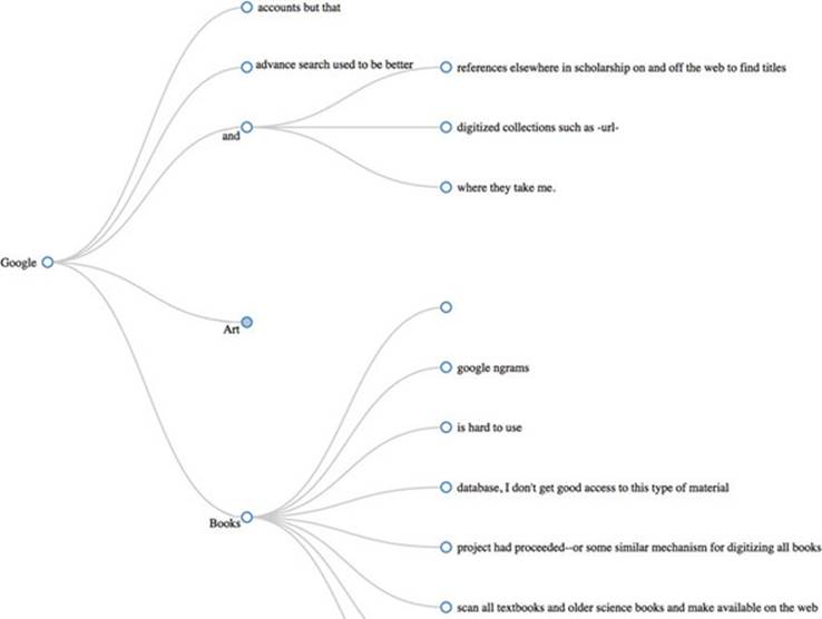
Figure 1.7. D3 has numerous SVG drawing functions (see chapter 4) so you can create your own custom visualizations, such as this representation of musical scores.

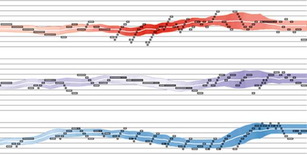
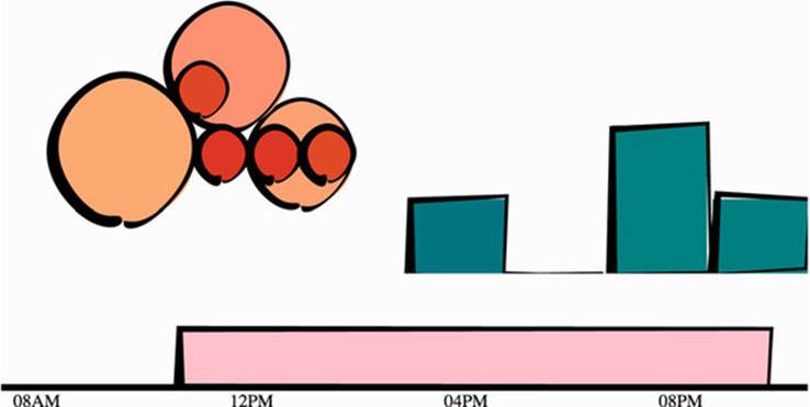
Figure 1.8. You can combine these layouts and functions to create a data dashboard like we’ll do in chapter 9. You can also use the drawing functions to make your bar charts look distinctive, such as this “sketchy” style.

Although the ability to create rich and varied graphics is one of D3’s strong points, more important for modern web development is the ability to embed the high level of interactivity that users expect. With D3, every element of every chart, from a spinning globe to a single, thin slice of a pie chart, is made interactive in the same way. And because D3 was written by someone well versed in data visualization practice, it includes a number of interactive components and behaviors that are standard in data visualization and web development.

You don’t invest your time learning D3 so that you can deploy Excel-style charts on the web. For that, there are easier, more convenient libraries. You learn D3 because it gives you the ability to implement almost every major data visualization technique. It also gives you the power to createyour own data visualization techniques, something a more general library can’t do.

For more examples of the variety of different data visualization techniques realized with D3, take a look at Christophe Viau’s gallery of over 2,000 D3 examples here: http://christopheviau.com/d3list/gallery.html.

By requiring a break with the practice of supporting long-obsolete browsers, D3.js affords developers the capacity to make not only richly interactive applications but also applications that are styled and served like traditional web content. This makes them more portable, more amenable to the growing, linked data web, and more easily maintained by large teams.

The decision on Bostock’s part to deal broadly with data, and to create a library capable of presenting maps as easily as charts, as easily as networks, as easily as ordered lists, also means that a developer doesn’t need to try to understand the abstractions and syntax of one library for maps, and another for dynamic text content, and another for data visualization. Instead, the code for running an interactive, force-directed network layout is very close to pure JavaScript and also similar to the code representing dynamic points of interest (POIs) on a D3.js map. Not only are the methods the same, but the very data could be the same, formulated in one way for lists and paragraphs and spans, while formulated in another way for geospatial representation. The class of data-driven documents is already broad and becomes even more all-encompassing when you also treat images and text as data.

1.2.2. D3 is about selecting and binding

Throughout this chapter, you’ll see code snippets that you can run in your browser to make changes to the graphical appearance of elements on your website. At the end of the chapter is an application written in D3 that explains the basics of the code we’re running in JavaScript. But before that we’ll explore the principles of web development using D3, and you’ll see this pattern of code over and over again: selecting.

Imagine we have a set of data, such as the price and size of a few houses, and a set of web page elements, whether graphics or traditional <div> elements, and that we want to represent the dataset, whether with text or through size and color. A selection is the group of all of them together, and we perform actions on the elements in the group, such as moving them, changing their color, or updating the values in the data. We work with the data and the web page elements separately, but the real power of D3 comes from using selections to combine data and web page elements.

Here’s a selection without any data:

d3.selectAll("circle.a").style("fill", "red").attr("cx", 100);

This takes every circle on our page with the class of "a" and turns it red and moves it so that its center is 100 pixels to the right of the left side of our <svg> canvas. Likewise, this code turns every div on our web page red and changes its class to "b":

d3.selectAll("div").style("background", "red").attr("class", "b");

But before we can change our circles and divs, we’ll need to create them, and before we do that, it’s best to understand what’s happening in this pattern.

The first part of that line of code, d3.selectAll(), is part of the core functionality necessary for understanding D3: selections. Selections can be made with d3.select(), which selects the first single element found, but more often you’ll use d3.selectAll(), which can be used to select multiple elements. Selections are a group of one or more web page elements that may be associated with a set of data, like the following code, which binds the elements in the array [1,5,11,3] to <div> elements with the class of "market":

d3.selectAll("div.market").data([1,5,11,3])

This association is known in D3 as binding data, and you can think of a selection as a set of web page elements and a corresponding, associated set of data. Sometimes there are more data elements than DOM elements, or vice versa, in which case D3 has functions designed to create or remove elements that you can use to generate content. We’ll cover selections and data-binding in detail in chapter 2. Selections might not include any data-binding, and won’t for most of the examples in this chapter, but the inclusion allows the powerful information visualization techniques of D3. You can make a selection on any elements in a web page, including items in a list, circles, or even regions on a map of Africa. Just as the elements can take a number of shapes, the data associated with those elements (where applicable) can take many forms.

1.2.3. D3 is about deriving the appearance of web page elements from bound data

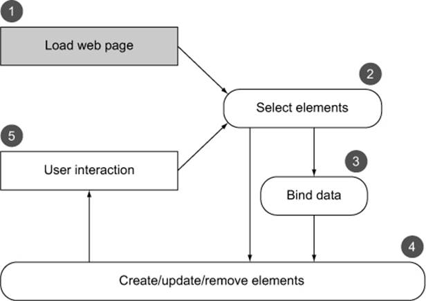
After you have a selection, you can then use D3 to modify the appearance of web page elements to reflect differences in the data. You may want to make the length of a line equal to the value of the data, or change the color to a particular color that corresponds to a class of data. You may want to hide or show elements as they correspond to a user’s navigation of a dataset. As you can see in figure 1.9, after the page has loaded, you use D3 to select elements and bind data for the purpose of creating, removing, or changing DOM elements. You continue to use this process in response to user interaction.

Figure 1.9. A page utilizing D3 is typically built in such a way that the page loads with styles, data, and content as defined in traditional HTML development with its initial display using D3 selections of HTML elements , either with data-binding or without it, to modify the structure and appearance of the page . The changes in structure prompt user interaction , which causes new selections with and without data-binding to further alter the page. Step 1 is shown differently because it only happens once (when you load the page), whereas every other step may happen multiple times, depending on user interaction.

You modify the appearance of elements by using selections to reference the data bound to an element in a selection. D3 iterates through the elements in your selection and performs the same action using the bound data, which results in different graphical effects. Although the action you perform is the same, the effect is different because it’s based on the variation in the data. You’ll see data-binding first at the end of this chapter, and in much more detail throughout this book.

1.2.4. Web page elements can now be divs, countries, and flowcharts

We’ve grown accustomed to thinking of web pages as consisting of text elements with containers for pictures, videos, or embedded applications. But as you grow more familiar with D3, you’ll begin to recognize that every element on the page can be treated with the same high-level abstractions. The most basic element on a web page, a <div> that represents a rectangle into which you can drop paragraphs, lists, and tables, can be selected and modified in the same way you can select and modify a country on a web map, or individual circles and lines that make up a complex data visualization.

To be able to select items on a web page, you have to ensure that they’re built in a manner that makes them a part of the traditional structure of a web page. You can’t select items in a Java applet, or in a Flash runtime, nor can you select the labels on an embedded Google map, but if you create these elements so that they exist as elements in your web page, then you give yourself tremendous flexibility. To get a taste of this, look at chapter 7, where we’ll build robust mapping applications in D3, and we’ll use the d3.select() syntax to update the appearance of a mapping application in the same manner as it’s being used here and elsewhere to create and move circles or <div> elements.

1.3. Using HTML5

We’ve come a long way from the days when animated GIFs and frames were the pinnacle of dynamic content on the web. In figure 1.10, you can see why GIFs never caught on for robust data visualization on the web. GIFs, like the infoviz libraries designed to use VML, are still necessary for earlier browsers, but D3 is designed for modern browsers that don’t need the helper libraries necessary for backward compatibility. D3 development isn’t for everyone, but if your audience can be assumed to have access to a modern web browser, D3 also brings a significant reduction in the cost necessary not only to code for older browsers but also to learn and keep updated on the various libraries that support backward compatibility with those older browsers.

Figure 1.10. Before GIFs were weaponized to share cute animal behavior, they were your only hope for animated data visualization on the web. Few examples from the 1990s like dpgraph.com exist, but this page has more than enough GIFs to remind us of their dangers.

A modern browser typically can not only display SVG graphics and obey CSS3 rules, but also has great performance. Along with Cascading Style Sheets (CSS) and Scalable Vector Graphics (SVG), we can break down HTML5 into the DOM and JavaScript. The following sections treat each of them and include code you can run to see how D3 uses their functionality to create interactive and dynamic web content.

1.3.1. The DOM

A web page is structured according to the DOM. You need a passing familiarity with the DOM to do web development, so we’ll take a quick look at DOM elements and structure in a simple web page in your browser and touch on the basics of the DOM. To get started, you’ll need a web server that you can access from the computer that you’re using to code. With that in place, you can download the D3 library from d3js.org (d3.js or d3.min.js for the minified version) and place that in the directory where you’ll make your web page. You’ll create a page called d3ia.html in the text editor with the following contents.

Listing 1.1. A simple web page demonstrating the DOM

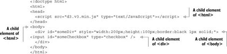
Basic HTML like this follows the DOM. It defines a set of nested elements, starting with an <html> element with all its child elements and their child elements and so on. In this example, the <script> and <body> elements are children of the <html> element, and the <div> element is a child of the <body> element. The <script> element loads the D3 library here, or it can have inline JavaScript code, whereas any content in the <body> element shows up onscreen when you navigate to this page.

UTF-8 and D3.js

D3 utilizes UTF-8 characters in its code, which means that you can do one of three things to make sure you don’t have any errors.

You can set your document to UTF-8:

<!DOCTYPE html><meta charset="utf-8">

Or you can set the charset of the script to UTF-8:

Or you can use the minified script, which shouldn’t have any UTF-8 characters in it:

Three categories of information about each element determine its behavior and appearance: styles, attributes, and properties. Styles can determine transparency, color, size, borders, and so on. Attributes typically refer to classes, IDs, and interactive behavior, though some attributes can also determine appearance, depending on which type of element you’re dealing with. Properties typically refer to states, such as the “checked” property of a check box, which is true if the box is checked and false if the box is unchecked. D3 has three corresponding functions to modify these values. If we wanted to modify the HTML elements in the previous example, we could use D3 functions that abstract this process:

d3.select("#someDiv").style("border", "5px darkgray dashed");

d3.select("#someDiv").attr("id", "newID");

d3.select("#someCheckbox").property("checked", true);

Like many D3 functions of this kind, if you don’t signify a new value, then the function returns the existing value. You’ll see this in action throughout this book, and later in the chapter as you write more code, but for now remember that these three functions allow you to change how an element appears and interacts.

The DOM also determines the onscreen drawing order of elements, with child elements drawn after and inside parent elements. Although you have some control over drawing elements above or below each other with traditional HTML using z-index, this isn’t available for SVG elements (though it might be implemented at some point using the render-order attribute).

Examining the DOM in the console

Navigate to d3ia.html, and you can get exposure to how D3 works. The page isn’t very impressive, with just a single, black-outlined rectangle. You could modify the look and feel of this web page by updating d3ia.html, but you’ll find that it’s easy to modify the page by using your web browser’s developer console. This is useful for testing changes to classes or elements before implementing them in your code. Open up the developer console, and you’ll have two useful screens, shown in figures 1.11 and 1.12, which we’ll go back to again and again.

Figure 1.11. The developer tools in Chrome place the JavaScript console on the rightmost tab, labeled “Console,” with the element inspector available using the hourglass on the bottom left or by browsing the DOM in the Elements tab.

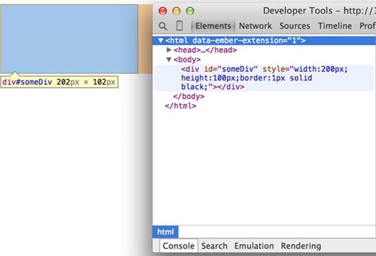
Figure 1.12. You can run JavaScript code in the console and also call global variables or declare new ones as necessary. Any code you write in the console and changes made to the web page are lost as soon as you reload the page.

Note

You’ll see the console in this first chapter, but in chapter 2, once you’re familiar with it, I’ll show only the output.

The element inspector allows you to look at the elements that make up your web page by navigating through the DOM (represented as nested text, where each child element is shown indented). You can also select an element onscreen graphically, typically represented as a magnifying glass or cursor icon.

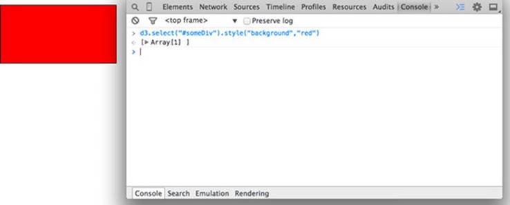
The other screen you’ll want to use quite often is the console (figure 1.12), which allows you to write and run JavaScript code right on your web page.

The examples in this book use Google Chrome and its developer console, but you could use Safari’s developer tools or Firebug in Firefox, or whatever developer console you’re most comfortable with. You can see and manipulate DOM elements such as <div> or <body> by clicking on the element inspector or looking at the DOM as represented in HTML. You can click one of these elements and change its appearance by modifying it in the console.

You can even delete elements in the console. Give it a try: select the div either in the DOM or visually, and press Delete. Now your web page is very lonely. Press Refresh so that your page reloads the HTML and your div comes back. You can adjust the size and color of your div by adding new styles or changing the existing one, so you can increase the width of the border and make it dashed by changing the border style to Black 5px Dashed. You can add content to the div in the form of other elements, or you can add text by right-clicking on the element and selecting Edit as HTML, as shown in figures 1.13 and 1.14.

Figure 1.13. Rather than adding or modifying individual styles and attributes, you have the ability to rewrite the HTML code as you would in a text editor. As with any changes, these only last until you reload the page.

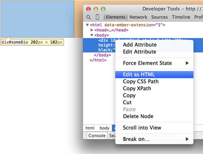
Figure 1.14. Changing the content of a DOM element is as simple as adding text between the opening and ending brackets of the element.

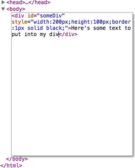
You can then write whatever you’d like in between the opening and closing HTML.

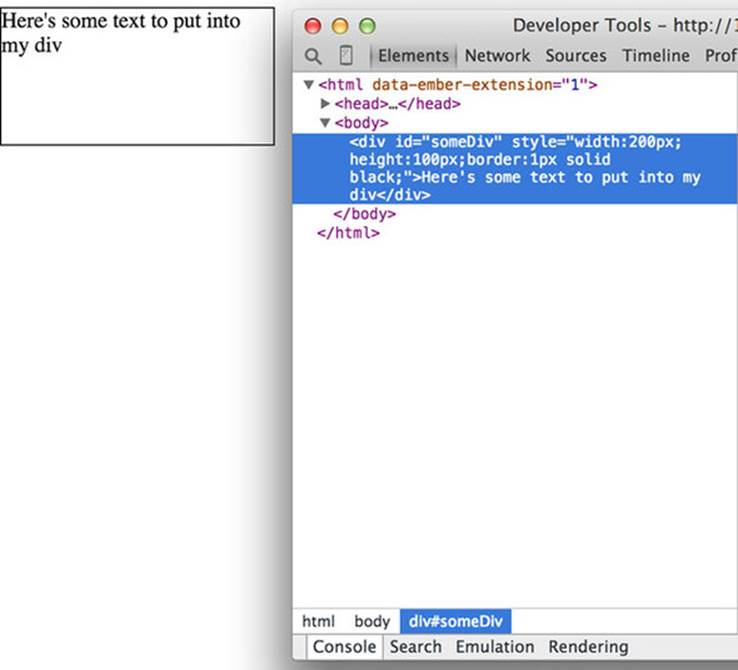
Any changes you make, regardless of whether they’re well structured or not, will be reflected on the web page. In figure 1.15 you see the results of modifying the HTML, which is rendered immediately on your page.

Figure 1.15. The page is updated as soon as you finish making your changes. Writing HTML manually in this way is only useful for planning how you might want to dynamically update the content.

In this way, you could slowly and painstakingly create a web page in the console. We’re not going to do that. Instead, we’ll use D3 to create elements on the fly with size, position, shape, and content based on our data.

1.3.2. Coding in the console

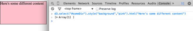
You’ll do a lot of your coding in the IDE of your choice, but one of the great things about web development is that you can test JavaScript code changes by using your console. Later you’ll focus on writing JavaScript, but for now, to demonstrate how the console works, copy the following code into your console and press Enter:

d3.select("div").style("background","lightblue").style("border", "solid black

1px").html("Something else maybe");

You should see the effect shown in figure 1.16.

Figure 1.16. The D3 select syntax modifies style using the .style() function, and traditional HTML content using the .html() function.

You’ll see a few more uses of traditional HTML elements in this chapter, and then again in chapter 3, but then you won’t see traditional DOM elements again until chapter 8, where we’ll use D3 to create complex, data-driven spreadsheets and galleries using <div>, <table>, and <select>elements. If all D3 could do was select HTML elements and change their style and content like this, then it wouldn’t be that useful for data visualization. To do more, we have to move away from traditional HTML and focus on a special type of element in the DOM: SVG.

1.3.3. SVG

A major value of HTML5 is the integrated support for SVG. SVG allows for simple mathematical representation of images that scale and are amenable to animation and interaction. Part of the attractiveness of D3 is that it provides an abstraction layer for drawing SVG. This is because SVG drawing can be a little confusing. SVG drawing instructions for complex shapes, known as <path> elements, are written a bit like the old LOGO programming language. You start at a point on a canvas and draw a line from that point to another. If you want it to curve, you can give the SVG drawing code coordinates on which to make that curve. So if you want to draw the line on the left, you’d create a <path> element in an <svg> canvas element in your web page, and you’d set the d attribute of that <path> element equal to the text on the right:

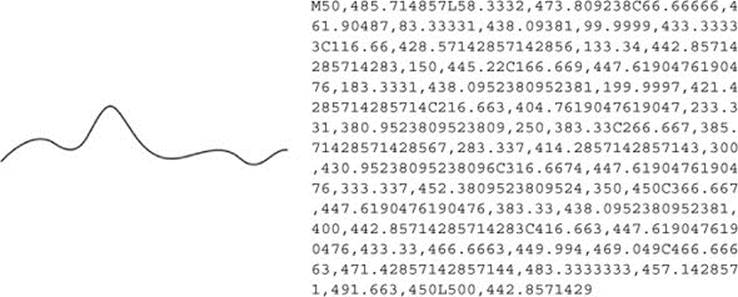
But you’d almost never want to create SVG by manually writing drawing instructions like this. Instead, you’ll want to use D3 to do the drawing with a variety of helper functions, or rely on other SVG elements that represent simple shapes (known as geometric or graphical primitives) using more readable attributes. You’ll start doing that in chapter 4, where you’ll use d3.svg.line and d3.svg.area to create line and area charts. For now, you’ll update d3ia.html to look like the following listing, which includes the necessary code for displaying SVG, as well as examples of the various shapes you might use.

Listing 1.2. A sample web page with SVG elements

<!doctype html>

<html>

</script>

<body>

<path d="M 10,60 40,30 50,50 60,30 70,80"

style="fill:black;stroke:gray;stroke-width:4px;" />

<polygon style="fill:gray;"

points="80,400 120,400 160,440 120,480 60,460" />

<g>

<line x1="200" y1="100" x2="450" y2="225"

style="stroke:black;stroke-width:2px;"/>

<rect x="410" y="200" width="100" height="50"

style="fill:pink;stroke:black;stroke-width:1px;" />

</g>

</svg>

</div>

</body>

</html>

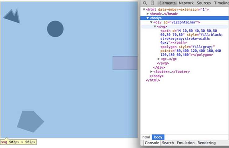
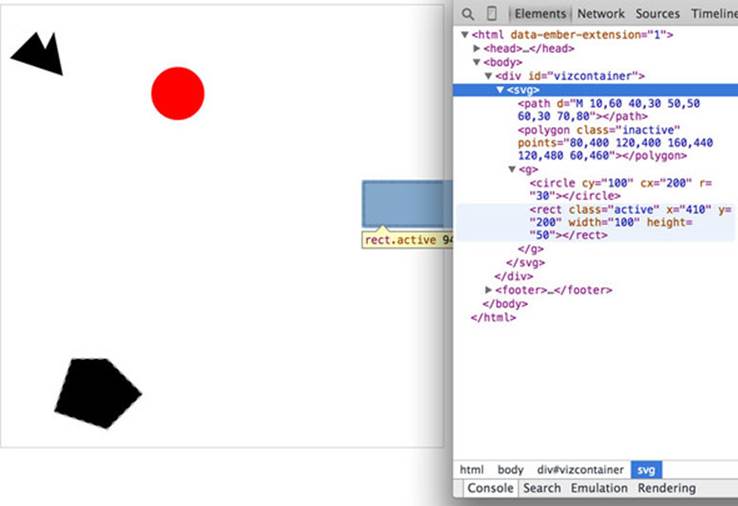
You can inspect the elements like you would the traditional elements we looked at earlier, as you can see in figure 1.17, and you can manipulate these elements using traditional JavaScript selectors like document.getElementById or with D3, removing them or changing the style like so:

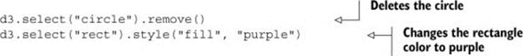
Figure 1.17. Inspecting the DOM of a web page with an SVG canvas reveals the nested graphical elements as well as the style and attributes that determine their position. Notice that the circle and rectangle exist as child elements of a group.

Now refresh your page and let’s take a look at the new elements. You’re familiar with divs, and it’s useful to put an SVG canvas in a div so you can access the parent container for layout and styling. Let’s take a look at each of the elements we’ve added.

<svg>

This is your canvas on which everything is drawn. The top-left corner is 0,0, and the canvas clips anything drawn beyond its defined height and width of 500,500 (the rectangle in our example). An <svg> element can be styled with CSS to have different borders and backgrounds. The <svg>element can also be dynamically resized using the viewBox attribute, which is more complex and beyond the scope of the overview here.

You can use CSS (which we’ll touch on later in this chapter) to style your SVG canvas or use D3 to add inline styles like so:

Note

The x-axis is drawn left-to-right, but the y-axis is drawn top-to-bottom, so you’ll see that the circle is set 200 pixels to the right and 100 pixels down.

<canvas>

There’s a second mode of drawing available with HTML5 using <canvas> elements to draw bitmaps. We won’t go into detail here, but you’ll see this method used in chapter 8 and again in chapter 11. The <canvas> element creates static graphics drawn in a manner similar to SVG that can then be saved as images. There are four main reasons to use canvas:

· Compatibility— We won’t worry about this because if you’re using D3, then you’re coding for a modern browser.

· Creating static images— You can draw your data visualization with canvas to save views as snapshots for thumbnail and gallery views (this is what we’ll do in chapter 8).

· Large amounts of data— SVG creates individual elements in the DOM, and although this is great for attaching events and styling, it can overwhelm a browser and cause significant slowdown (this is what we’ll use canvas for in chapter 11).

· WebGL— The <canvas> element allows you to use WebGL to draw, so that you can create 3D objects. You can also create 3D objects like globes and polyhedrons using SVG, which we’ll get into a bit in chapter 7 as we examine geospatial information visualization.

<Circle>, <Rect>, <Line>, <Polygon>

SVG óprovides a set of common shapes, each of which has attributes that determine their size and position to make them easier to deal with than the generic d attribute you saw earlier. These attributes vary depending on the element that you’re dealing with, so that <rect> has x and yattributes that determine the shape’s top-left corner, as well as height and width attributes that determine its overall form. In comparison, the <circle> element has cx and cy attributes that determine the center of the circle, and an r attribute that determines the radius of the circle. The<line> element has x1 and y1 attributes that determine the starting point of the line and x2 and y2 attributes that determine its end point. There are other simple shapes that are similar to these, such as the <ellipse>, and there are more complex shapes, like the <polygon> with apoints attribute that holds a set of comma-separated xy coordinates, in clockwise order, that determines the area bounded by the polygon.

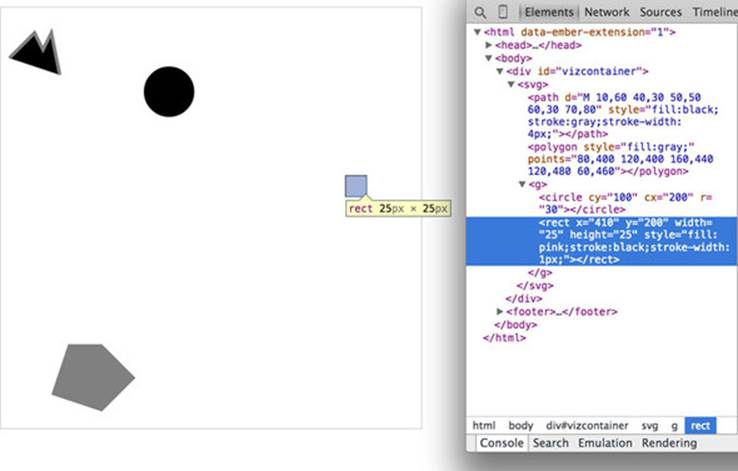
Each of these attributes can be hand-edited in HTML to adjust its size, form, and position. Open up your element inspector, and click the <rect>. Change its width to 25 and its height to 25, as shown in figure 1.18.

Figure 1.18. Modifying the height and width attributes of a <rect> element changes the appearance of that element. Inspecting the element also shows how the stroke adds to the computed size of the element.^[¹^]

¹ Figures that have a picture icon at the end of the caption, like figure 1.18, have an online example that you can work with interactively or download to run locally. Click on the icon in the eBook version of the book, or go to manning.com/meeks to find all interactive examples online.

Infoviz term: geometric primitive

Accomplished artists can draw anything with vector graphics, but you’re probably not looking at D3 because you’re an artist. Instead, you’re dealing with graphics and have more pragmatic goals in mind. From that perspective, it’s important to understand the concept of geometric primitives (also known as graphical primitives). Geometric primitives are simple shapes such as points, lines, circles, and rectangles. These shapes, which can be combined to make more complex graphics, are particularly useful for visually displaying information.

Primitives are also useful for understanding complex information visualizations that you see out in the real world. Dendrograms like the one shown in figure 1.20 are far less intimidating when you realize they’re just circles and lines. Interactive timelines are easier to understand and create when you think of them as collections of rectangles and points. Even geographic data, which primarily comes in the form of polygons, points, and lines, is less confusing when you break it down into its most basic graphical structures.

Now you’ve learned why there’s no SVG <square>. The color, stroke, and transparency of any shape can be changed by adjusting the style of the shape, with "fill" determining the color of the area of the shape and "stroke", "stroke-width", "stroke-dasharray" determining its outline.

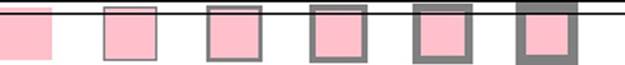
Notice, though, that the inspected element has a measurement of 27 px x 27 px. That’s because the 1-px stroke is drawn on the outside of the shape. That makes sense, once you know the rule, but if you change the "stroke-width" to "2px" it will still be 27 px x 27 px. That’s because the stroke is drawn evenly over the inside and outside borders as seen in figure 1.19. This may not seem too big a deal, but it’s something to remember when you’re trying to line up your shapes later on.

Figure 1.19. The same 25 x 25 <rect> with no, 1-px, 2-px, 3-px, 4-px, and 5-px strokes. Though these are drawn on a retina screen using half-pixels, the second and third report the same width and height (27 px x 27 px) as the fourth and fifth (29 px x 29 px).

Change the style parameters of the rectangle to the following:

"fill:purple;stroke-width:5px;stroke:cornflowerblue;"

Congratulations! You’ve now successfully visualized the complex and ambiguous phenomenon known as “ugly.”

<text>

SVG provides the capacity to write text as well as shapes. SVG text, though, doesn’t have the formatting support found in HTML elements, and so it’s primarily used for labels. If you do want to do basic formatting, you can nest <tspan> elements in <text> elements.

<g>

The <g> or group element is distinct from the SVG elements we’ve discussed in that it has no graphical representation and doesn’t exist as a bounded space. Instead, it’s a logical grouping of elements. You’ll want to use <g> elements extensively when creating graphical objects that are made up of several shapes and text. For instance, if you wanted to have a circle with a label above it and move the label and the circle at the same time, then you’d place them inside a <g> element:

<g>

<text>This circle's Label</text>

</g>

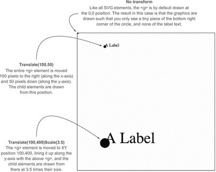
Moving a <g> around your canvas requires you to adjust the transform attribute of the <g> element. The transform attribute is more intimidating than the various xy attributes of shapes, because it accepts a structured description in text of how you want to transform a shape. One of those structures is translate(), which accepts a pair of coordinates that move the element to the xy position defined by the values in translate(x,y). So if you want to move a <g> element 100 pixels to the right and 50 pixels down, then you need to set its transform attribute totransform="translate(100,50)". The transform attribute also accepts a scale() setting so you can change the rendered scale of the shape. You can see these settings in action by modifying the previous example with the results shown in figure 1.20.

Figure 1.20. All SVG elements can be affected by the transform attribute, but this is particularly salient when working with <g> elements, which require this approach to adjust their position. The child elements are drawn by using the position of their parent <g> as their relative 0,0 position. The scale() setting in the transform attribute then affects the scale of any of the size and position attributes of the child elements.

Listing 1.3. Grouping SVG elements

<g>

<text>This circle's Label</text>

</g>

<text>This circle's Label</text>

</g>

<text>This circle's Label</text>

</g>

<path>

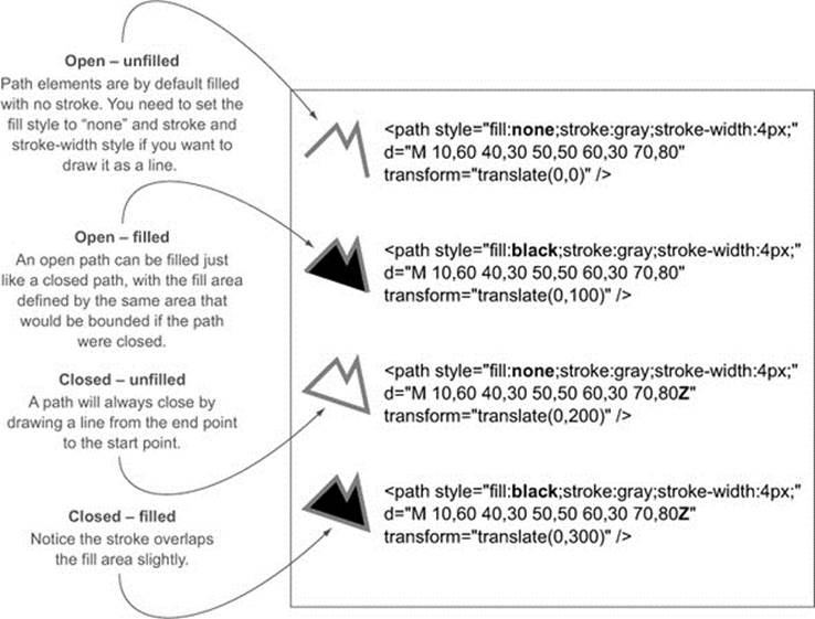
A path is an area determined by its d attribute. Paths can be open or closed, meaning the last point connects to the first if closed and doesn’t if open. The open or closed nature of a path is determined by the absence or presence of the letter Z at the end of the text string in the d attribute. It can still be filled either way. You can see the difference in figure 1.21.

Figure 1.21. Each path shown here uses the same coordinates in its d attribute, with the only differences between them being the presence or absence of the letter Z at the end of the text string defining the d attribute, the settings for fill and stroke, and the position via the transform attribute.

Listing 1.4. SVG path fill and closing

<path style="fill:none;stroke:gray;stroke-width:4px;"

d="M 10,60 40,30 50,50 60,30 70,80" transform="translate(0,0)" />

<path style="fill:black;stroke:gray;stroke-width:4px;"

d="M 10,60 40,30 50,50 60,30 70,80" transform="translate(0,100)" />

<path style="fill:none;stroke:gray;stroke-width:4px;"

d="M 10,60 40,30 50,50 60,30 70,80Z" transform="translate(0,200)" />

<path style="fill:black;stroke:gray;stroke-width:4px;"

d="M 10,60 40,30 50,50 60,30 70,80Z" transform="translate(0,300)" />

Although sometimes you may want to write that d attribute yourself, it’s more likely that your experience crafting SVG will come in one of three ways: using geometric primitives like circles, rectangles, or polygons; drawing SVG using a vector graphics editor like Adobe Illustrator or Inkscape; or drawing SVG parametrically using handwritten constructors or built-in constructors in D3. Most of this book focuses on using D3 to create SVG, but don’t overlook the possibility of creating SVG using an external application or another library and then manipulating them using D3 like we’ll do using d3.html in chapter 3.

1.3.4. CSS

CSS are used to style the elements in the DOM. A style sheet can exist as a separate .css file that you include in your HTML page or can be embedded directly in the HTML page. Style sheets refer to an ID, class, or type of element and determine the appearance of that element. The terminology used to define the style is a CSS selector and is the same type of selector used in the d3.select() syntax. You can set inline styles (that are applied to only a single element) by using d3.select("#someElement") .style("opacity", .5) to set the opacity of an element to 50%. Let’s update your d3ia.html to include a style sheet.

Listing 1.5. A sample web page with a style sheet

<!doctype html>

<html>

<style>

.inactive, .tentative {

stroke: darkgray;

stroke-width: 2px;

stroke-dasharray: 5 5;

}

.tentative {

opacity: .5;

}

.active {

stroke: black;

stroke-width: 4px;

stroke-dasharray: 1;

}

circle {

fill: red;

}

rect {

fill: darkgray;

}

</style>

<body>

<g>

</g>

</svg>

</div>

</body>

</html>

The results stack on each other, so when you examine the rectangle element, as shown in figure 1.22, you see that its style is set by the reference to rect in the style sheet as well as the class attribute of active.

Figure 1.22. Examining an SVG rectangle in the console shows that it inherits its fill style from the CSS style applied to <rect> types and its stroke style from the .active class.

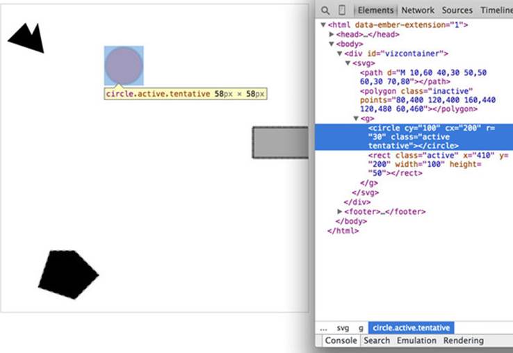
Style sheets can also refer to a state of the element, so with :hover you can change the way an element looks when the user mouses over that element. You can learn about other complex CSS selectors in more detail in a book devoted to that subject. For this book, we’ll focus mostly on using CSS classes and IDs for selection and to change style. The most useful way to do this is to have CSS classes associated with particular stylistic changes and then change the class of an element. You can change the class of an element, which is an attribute of an element, by selecting and modifying the class attribute. The circle shown in figure 1.23 is affected by two overlapping classes: .active and .tentative.

Figure 1.23. The SVG circle has its fill value set by its type in the style sheet, with its opacity set by its membership in the .tentative class and its stroke set by its membership in the .active class. Notice that the stroke settings from the .tentative class are overwritten by the stroke settings in the later declared .active class.

In listing 1.5 we see a couple of possibly overlapping classes, with tentative, active, and inactive all applying different style changes to your shape (such as the highlighted circle in figure 1.23). When an element needs only be assigned to one of these classes, you can overwrite the class attribute entirely:

d3.select("circle").attr("class", "tentative");

The results, as shown in figure 1.24, are what we would expect. This overwrites the entire class attribute to the value you set. But elements can have multiple classes, and sometimes an element is both active and tentative or inactive and tentative, so let’s reload the page and take advantage of the helper function d3.classed(), which allows you to add or remove a class from the classes in an element:

d3.select("circle").classed("active", true);

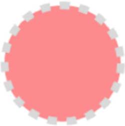
Figure 1.24. An SVG circle with fill style determined by its type and its opacity and stroke settings determined by its membership in the tentative class.

By using .classed(), you don’t overwrite the existing attribute, but rather append or remove the named class from the list. You can see the results of two classes with conflicting styles defined. The active style overwrites the tentative style because it occurs later in the style sheet. Another rule to remember is that more specific rules overwrite more general rules. There’s more to CSS, but this book won’t go into that.

By defining style in your style sheet and changing appearance based on class membership, you create code that’s more maintainable and readable. You’ll need to use inline styles to set the graphical appearance of a set of elements to a variety of different values, for example, changing the fill color to correspond to a color ramp based on the data bound to that set of elements. You’ll see that functionality in action later when you deal with bound data. But as a general rule, setting inline styles should only be used when you can’t use traditional classes and states defined in a style sheet.

1.3.5. JavaScript

D3, like many information visualization libraries in JavaScript, provides functions to abstract the process of creating and modifying web page elements. On top of that, it provides mechanisms to link data and web page elements in a way that makes the drawing and updating of these SVG elements reusable and maintainable. But these mechanisms are also applicable to more traditional HTML elements like paragraphs and divs.

As a result, a web application written in D3 can accomplish much of the UI functionality that users expect without relying on libraries like jQuery. This is because the latest version of JavaScript has built-in functionality that used to be available only with jQuery. If you read the solutions on Stack Overflow, you may think that being a JavaScript developer requires being a jQuery developer, but unless you’re developing for an audience that uses a browser that won’t support the key features of D3, or you need to use a plugin that requires jQuery, then you might just as easily write the same functionality in JavaScript.

When writing JavaScript with D3, you should familiarize yourself with two subjects: method chaining and arrays.

Method chaining

D3 examples, like many examples written in JavaScript, use method chaining extensively. Method chaining, also known as function chaining, is facilitated by returning the method itself with the successful completion of functions associated with a method. One way to think of method chaining is to think of how we talk and refer to each other. Imagine you were talking to someone at a party, and you asked about another guest:

· “What’s her name?”

· “Her name is Lindsay.”

· “Where does she work?”

· “She works at Tesla.”

· “Where does she live?”

· “She lives in Cupertino.”

· “Does she have any children?”

· “Yes, she has a daughter.”

· “What’s her name?”

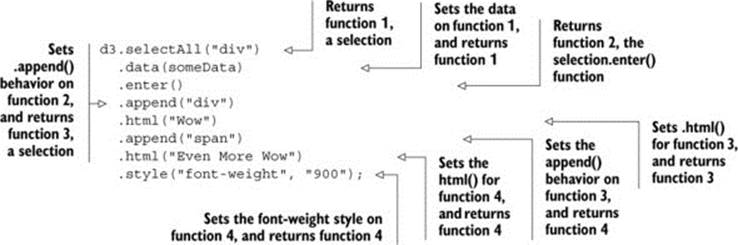
Do you think the answer to that last question would be “Lindsay”? Of course not. You’d expect the answer to refer to Lindsay’s daughter, even though all the previous questions referred to Lindsay. Method chaining is like that. It returns the same function as long as you use getter and setter methods of that function, and returns the new function when you call a method that creates something new. Method chaining is used a lot in D3 examples, which means you’ll see something like this written on one line or formatted (but functionally identical) to something written on multiple lines:

d3.selectAll("div").data(someData).enter().append("div").html("Wow").append("

span").html("Even More Wow").style("font-weight", "900");

That line is the same as the following code. The only change is in the use of line breaks, which JavaScript ignores:

You could write each line separately, declaring the different variables as you go, and achieve the same effect. That might make more sense if you haven’t been exposed to method chaining before.

var function1 = d3.selectAll("div");

var function1withData = function1.data(someData);

var function2 = function1withData.enter();

var function3 = function2.append("div");

function3.html("Wow");

var function4 = function3.append("span");

function4.html("Even More Wow");

function4.style("font-weight", "900");

You can see this when you run the code in your console. This is the first time you’ve used the .data() function, which along with .select() is at the core of developing with D3. When you use .data(), you bind each element in your selection to each item in an array. If you have more items in your array than elements in your selection, then you can use the .enter() function to define what to do with each extra element. In the previous function, you select all the <div> elements in the <body> and the .enter() function tells D3 to .append() a new div when there are more elements in the array than elements in the selection. Given that your d3ia.html page already has one div, if you bind an array with more than one value, D3 appends, or adds, a div for each value in the array beyond the first.

A corresponding .exit() function defines how to respond when an array has fewer values than a selection. For now, you’ll run the code as it appears in the examples, and in later chapters we’ll get into much more detail on the way selections and binding work.

With this example, you’re not doing anything with the data in the array and only creating elements based on the size of the array (one <div> for each element in the array). This example assumes that you already have a <div> in your html with a black border (as seen in figure 1.25). Here’s the HTML that would get that done:

<!doctype html>

<html>

<style>

#borderdiv {

width: 200px;

height: 50px;

border: 1px solid gray;

}

</style>

<body>

</body>

</html>

Figure 1.25. By binding an array of four values to a selection of <div> elements on the page, the .enter() function created three new <div> elements to reflect the size mismatch between the data array and the selection.

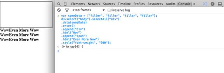
For this to work, you need to give someData a value. With that in place, you can run your code:

var someData = ["filler", "filler", "filler", "filler"];

d3.select("body").selectAll("div")

.data(someData)

.enter()

.append("div")

.html("Wow")

.append("span")

.html("Even More Wow")

.style("font-weight", "900");

The result, as shown in figure 1.25, is the addition of three lines of text. It might surprise you that this code is three lines, given that the array has four values. Although the data was bound to the existing <div> element on the page, the actions that changed the contents were only applied to the .enter() function. They were only applied to the newly created <div> elements that were “entering” the DOM for the first time.

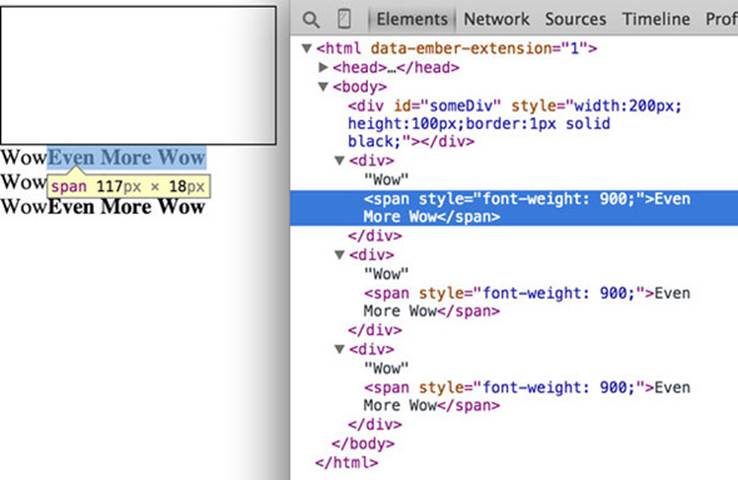
When you inspect the DOM, as shown in figure 1.26, you see that the method chaining operated in the manner just described. A <div> was added, and its HTML content was set to "Wow". A <span> element with a different style was appended to the <div>, and its HTML content was set to "Even More Wow". There’s more you can do, but first you need to examine the array object you’re binding, and focus on JavaScript arrays and array functions.

Figure 1.26. Inspecting the DOM shows that the new <div> elements have been created with unformatted content followed by the child <span> element with style and content set by your code.

Arrays and array functions

D3 is all about arrays, and so it’s important to understand the structure of arrays and the options available to you to prepare those arrays for binding to data. Your array might be an array of string or number literals, such as this:

someNumbers = [17, 82, 9, 500, 40];

someColors = ["blue", "red", "chartreuse", "orange"];

Or it may be an array of JSON objects, which will become more common as you do more interesting things with D3:

somePeople = [{name: "Peter", age: 27}, {name: "Sulayman", age: 24},

{name: "K.C.", age: 49}];

One example of a useful array function is .filter(), which returns an array whose elements satisfy a test you provide. For instance, here’s how to create an array out of someNumbers that had values greater than 40:

someNumbers.filter(function(el) {return el >= 40});

Likewise, here’s how you could create an array out of someColors with names shorter than five letters:

someColors.filter(function(el) {return el.length < 5});

The function .filter() is a method of an array and accepts a function that iterates through the array with the variable you’ve named. In this function, you name that variable el, and the function runs a test on each value by testing on el. When that test evaluates true, the element is kept in our new array.

The result of this .filter() function, which you can see in figure 1.27, returns either the element or nothing (depending on if it satisfies the test), building a new array consisting only of the elements that do.

Figure 1.27. Running JavaScript in the console allows you to test your code. Here you’ve created a new array called smallerNumbers that consists of only three values, which you can then use as your data in a selection to update and create new elements.

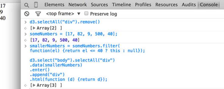
smallerNumbers = someNumbers.filter(

function(el) {return el <= 40 ? this : null});

d3.select("body").selectAll("div")

.data(smallerNumbers)

.enter()

.append("div")

.html(function (d) {return d});

The resulting code creates two new divs from your three-value array smallerNumbers. (Remember that one div already exists, and so the .enter() function doesn’t trigger even though data is bound to that existing div.) The contents of the div are the values in your array. This is done through an anonymous function (sometimes referred to in D3 examples as an accessor) in your .html() function and is another key aspect of D3. Any anonymous function called when setting the .style(), .attr(), .property(), .html(), or other function of a selection can provide you with the data bound to that selection. As you explore examples, you’ll see this function deployed again and again:

.style("background", function(d,i) {return d})

.attr("cx", function(d,i) {return i})

.html(function(d,i) {return d})

In every case, the first variable (typically represented with the letter d, but you can declare it as whatever you want) contains the data value bound to that element, and the second variable returns the array position (known as an index, hence the variable name i) of the value bound to that element. This may seem a bit strange, but you’ll get used to it as you see it used in a variety of ways in the upcoming chapters.

JavaScript has many other array functions, and you can do much more than we covered here, but that’s the subject of several other books. It’s time to look at the kinds of data you’ll work with.

1.4. Data standards

Standardization of methods of displaying data has been fed by and feeds into standardization of methods of formatting that data. Data can be formatted in a variety of manners for a variety of purposes, but it tends to fall into a few recognizable classes: tabular data, nested data, network data, geographic data, raw data, and objects.

1.4.1. Tabular data

Tabular data appears in columns and rows typically found in a spreadsheet or a table in a database. Although you invariably end up creating arrays of objects in D3, it’s often more efficient and easier to pull in data in tabular format. Tabular data is delimited with a particular character, and that delimiter determines its format. You can have Comma-Separated Values (CSV), where the delimiter is a comma, or tab-delimited values, or a semicolon or a pipe symbol acting as the delimiter. For instance, you may have a spreadsheet of user information that includes age and salary. If you export it in a delimited form, it will look like table 1.1.

Table 1.1. Delimited data can be expressed in different forms. Here a dataset stores name, age, and salary of two people using commas, spaces, or the bar symbol to delimit the different fields.

name,age,salary	name age salary	name\|age\|salary
Sal,34,50000	Sal 34 50000	Sal\|34\|50000
Nan,22,75000	Nan 22 75000	Nan\|22\|75000

D3 provides three different functions to pull in tabular data: d3.csv(), d3.tsv(), and d3.dsv(). The only difference between them is that d3.csv() is built for comma-delimited files, d3.tsv() is built for tab-delimited files, and d3.dsv() allows you to declare the delimiter. You’ll see them in action throughout the book.

1.4.2. Nested data

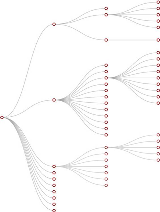
Data that is nested, with objects existing as children of objects recursively, is very common. Many of the most intuitive layouts in D3 are based on nested data, which can be represented as trees, such as the one in figure 1.28, or packed in circles or boxes. Data isn’t often output in such a format, and requires a bit of scripting to organize it as such, but the flexibility of this representation is worth the effort. You’ll see hierarchical data in detail in chapter 5 when we look at various popular D3 layouts.

Figure 1.28. Nested data represents parent/child relationships of objects, typically with each object having an array of child objects, and is represented in a number of forms, such as this dendrogram. Notice that each object can have only one parent.

1.4.3. Network data

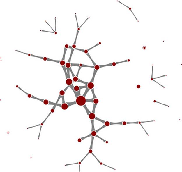
Networks are everywhere. Whether they’re the raw output of social networking streams, transportation networks, or a flowchart, networks are a powerful method of delivering an understanding of complex systems. Networks are often represented as node-link diagrams, as shown in figure 1.29. Like geographic data, network data has many standards, but this text focuses only on two forms: node/edge lists and connected arrays. Network data can also be easily transformed into these data types by using a freely available network analysis tool like Gephi (available at gephi.org). We’ll examine network data and network data standards when we deal with network visualization in chapter 6.

Figure 1.29. Network data consists of objects and the connections between them. The objects are typically referred to as nodes or vertices, while the connections are referred to as edges or links. Networks are often represented using force-directed algorithms, such as the example here, that arrange the network in such a way as to pull connected nodes toward each other.

1.4.4. Geographic data

Geographic data refers to locations either as points or shapes, and is used to create the variety of online maps seen on the web today, such as the map of the United States in figure 1.30. The incredible popularity of web mapping means that you can get access to a massive amount of publicly accessible geodata for any project. Geographic data has a few standards, but the focus in this book is on two: the GeoJSON and TopoJSON standards. Although geodata may come in many forms, readily available geographic information systems (GIS) tools like Quantum GIS allow developers to transform it into GIS format for ready delivery to the web. We’ll look at geographic data closely in chapter 7.

Figure 1.30. Geographic data stores the spatial geometry of objects, such as states. Each of the states in this image is represented as a separate feature with an array of values indicating its shape. Geographic data can also consist of points, such as for cities, or lines, such as for roads.

1.4.5. Raw data

As you’ll see in chapter 2, everything is data, including images or blocks of text. Although information visualization typically uses shapes encoded by color and size to represent data, sometimes the best way to represent it in D3 is with linear narrative text, an image, or a video. If you develop applications for an audience that needs to understand complex systems, but you consider the manipulation of text or images to be somehow separate from the representation of numerical or categorical data as shapes, then you arbitrarily reduce your capability to communicate. The layouts and formatting used when dealing with text and images, typically tied to older modes of web publication, are possible in D3, and we’ll deal with that throughout this book, but especially in chapter 8.

1.4.6. Objects

You’ll use two types of data points with D3: literals and objects. A literal, such as a string literal like "Apple" or "beer" or a number literal like 64273 or 5.44, is straightforward. A JavaScript object, expressed using JavaScript Object Notation (JSON), isn’t so straightforward, but is something that you need to understand if you plan to do sophisticated data visualization.

Let’s say you have a dataset that consists of individuals from an insurance database, and you need to know how old someone is, whether they’re employed, their name, and their children, if any. A JSON object that represents each individual in such a database would be expressed as follows:

{name: "Charlie", age: 55, employed: true, childrenNames: ["Ruth", "Charlie

Jr."]}

Each object is surround by braces, {}, and has attributes that have a string, number, array, boolean, or object as their value. You can assign an object to a variable and access its attributes by referring to them, like so:

var person = {name: "Charlie", age: 55, employed: true, childrenNames:

["Ruth", "Charlie Jr."]};

person.name // Charlie

person["name"] // Charlie

person.name = "Charles" // Sets name to Charles

person["name"] = "Charles" // Sets name to Charles

person.age < 65 // true

person.childrenNames // ["Ruth", "Charlie Jr."]

person.childrenNames[0] // "Ruth"

Objects can be stored in arrays and associated with elements using d3.select() syntax. But objects can also be iterated through like arrays using a for loop:

for (x in person) {console.log(x); console.log(person[x]);}

The x in the loop represents each attribute in the person object. Each x will be one of the attributes such as name, age, and so on This allows you to iterate through the attributes using person[x] to show the value of that attribute of the object.

If your data is stored as JSON, then you can import it using d3.json(), which you’ll see many times in later chapters. But remember that whenever you use d3.csv(), D3 imports the data as an array of JSON objects. We’ll look at objects more extensively as we use them later.

1.5. Infoviz standards expressed in D3

Information visualization has never been so popular as it is today. The wealth of maps, charts, and complex representations of systems and datasets isn’t just present in the workplace, but also in our entertainment and everyday lives. With this popularity comes a growing library of classes and subclasses of representation of data and information using visual means, as well as aesthetic rules to promote legibility and comprehension. Your audience, whether the general public, academics, or decision makers, has grown accustomed to what we once considered incredibly abstract and complicated representations of trends in data. This is why libraries like D3 are popular not only among data scientists, but also among journalists, artists, scholars, IT professionals, and even fan communities.

But the wealth of options can seem overwhelming, and the relative ease of modifying a dataset to appear in a streamgraph, treemap, or histogram tends to promote the idea that information visualization is more about style than substance. Fortunately, well-established rules dictate what charts and methods to use for different types of data from different systems. Although we can’t cover every rule in the book, we’ll touch on ones that are useful to consider as we create more complicated information visualizations. Although some developers use D3 to revolutionize the use of color and layout, most simply want to create visual representations of data that support practical concerns. Because D3 is being developed in this mature information visualization environment, it contains numerous helper functions to let developers worry about interface and design rather than color and axes.

Still, to properly deploy information visualization, you should know what to do and what not to do. The best way to learn this is to review the work of established designers and information visualization practitioners, and you need to have a firm understanding not only of your data but of your audience. Although an entire library of works deals with these issues, here are a few that I’ve found useful and can get you oriented on the basics:

· The Visual Display of Quantitative Information Envisioning Information, Edward Tufte

· Designing for Information, Isabel Meirelles

· Pattern Recognition, Christian Swinehart

These are by no means the only or most applicable texts for learning data visualization, but I’ve found them useful for getting started. You should pare down and establish fundamental, even basic, data visualization practices that clearly represent the trends that are salient to your audience. When in doubt, simplify—it’s often better to present a histogram than a streamgraph, or a hierarchical network layout (like a dendrogram) than a force-directed one. The more visually complex methods of displaying data tend to inspire more excitement, but can also lead an audience to see what they want to see or focus on the aesthetics of the graphics rather than the data.

Infoviz tip: kill your darlings

One of the best pieces of advice when it comes to working in information visualization comes from the practice of writing: “Kill your darlings.” Just as writers may become enamored of certain scenes or characters, you can become enamored of a particularly elegant or sophisticated-looking graphic. Your love of a cool chart or animation can distract you from the goal of communicating the structure and patterns in the data. Remember to save your harshest criticism for your most beloved pieces, because you may find, much to your chagrin, that they’re not as useful and informative as you think they are.

One thing to keep in mind while reading about data visualization is that the literature is often focused on static charts. With D3 you’ll be making interactive and dynamic visualizations and not just static ones. You’ll make a dynamic (or animated) data visualization before you finish this chapter, and using D3 to make a chart interactive is incredibly simple. A few interactive touches can make a visualization not only more readable but significantly more engaging. Users who feel like they’re exploring rather than reading, even if only with a few mouseover events or a simple click to zoom, will find the content of the visualization more compelling than in a static page. But this added complexity requires an investment in learning principles of interface design and user experience. We’ll get into this in more detail in chapters 9 and 12.

1.6. Your first D3 app

Throughout this chapter, you’ve seen various lines of code and the effect of those lines of code on the growing d3ia.html sample page you’ve been building. But I’ve avoided explaining the code in too much detail so that you could concentrate on the principles at work in D3. It’s simple to build an application from scratch that uses D3 to create and modify elements. Let’s put it all together and see how it works. First, let’s start with a clean HTML page that doesn’t have any defined styles or existing divs.

Listing 1.6. A simple webpage

<!doctype html>

<html>

<head>

</head>

<body>

</body>

</html>

1.6.1. Hello world with divs

We can use D3 as an abstraction layer for adding traditional content to the page. Although we can write JavaScript inside our .html file or in its own .js file, let’s put code in the console and see how it works. Later, we’ll focus on the various commands in more detail for layouts and interfaces. We can get started with a piece of code that uses D3 to write to our web page.

Listing 1.7. Using d3.select to set style and HTML content

d3.select("body").append("div")

.style("border", "1px black solid")

.html("hello world");

We can adjust the element on the page and give it interactivity with the inclusion of the .on() function.

Listing 1.8. Using d3.select to set attributes and event listeners

d3.select("div")

.style("background-color", "pink")

.style("font-size", "24px")

.attr("id", "newDiv")

.attr("class", "d3div")

.on("click", function() {console.log("You clicked a div")});

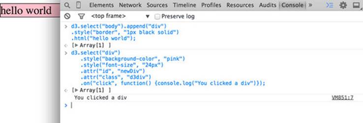
The .on() function allows us to create an event listener for the currently selected element or set of elements. It accepts the variety of events that can happen to an element, such as click, mouseover, mouseout, and so on. If you click your div, you’ll notice that it gives a response in your console, as shown in figure 1.31.

Figure 1.31. Using console.log(), you can test to see if an event is properly firing. Here you create a <div> and assign an onclick event handler using the .on() syntax. When you click that element and fire the event, the action is noted in the console.

1.6.2. Hello World with circles

You didn’t pick up this book to learn how to add divs to a web page, but you likely want to deal with graphics like lines and circles. To append shapes to a page with D3, you need to have an SVG canvas element somewhere in your page’s DOM. You could either add this SVG canvas to the page as you write the HTML, or you could append it using the D3 syntax you’ve learned:

d3.select("body").append("svg");

Let’s adjust our d3ia.html page to start with an SVG canvas.

Listing 1.9. A simple web page with an SVG canvas

<!doctype html>

<html>

<head>

</head>

<body>

</div>

</body>

</html>

After we have an SVG canvas on our page, we can append various shapes to it using the same select() and append() syntax we’ve been using in section 1.6.1 for <div> elements.

Listing 1.10. Creating lines and circles with select and append

d3.select("svg")

.append("line")

.attr("x1", 20)

.attr("y1", 20)

.attr("x2",400)

.attr("y2",400)

.style("stroke", "black")

.style("stroke-width","2px");

d3.select("svg")

.append("text")

.attr("x",20)

.attr("y",20)

.text("HELLO");

d3.select("svg")

.append("circle")

.attr("r", 20)

.attr("cx",20)

.attr("cy",20)

.style("fill","red");

d3.select("svg")

.append("circle")

.attr("r", 100)

.attr("cx",400)

.attr("cy",400)

.style("fill","lightblue");

d3.select("svg")

.append("text")

.attr("x",400)

.attr("y",400)

.text("WORLD");

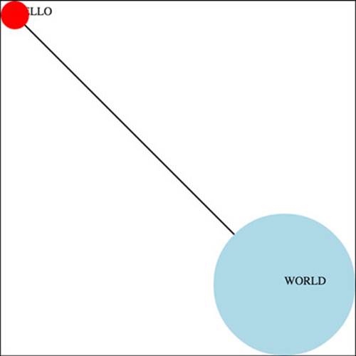
Notice that your circles are drawn over the line and the text is drawn above or below the circle, depending on the order in which you run your commands, as you can see in figure 1.32. This is because the draw order of SVG is based on its DOM order. Later you’ll learn some methods to adjust that order.

Figure 1.32. The result of running listing 1.10 in the console is the creation of two circles, a line, and two text elements. The order in which these elements are drawn results in the first label covered by the circle drawn later.

1.6.3. A conversation with D3

Writing Hello World with languages is such a common example that I thought we should give the world a chance to respond. Let’s add the same big circle and little circle from before, but this time, when we add text, we’ll include the .style ("opacity") setting that makes our text invisible. We’ll also give each text element a .attr("id") setting so that the text near the small circle has an id attribute with the value of "a", and the text near the large circle has an id attribute with the value of "b".

Listing 1.11. SVG elements with IDs and transparency

d3.select("svg")

.append("circle")

.attr("r", 20)

.attr("cx",20)

.attr("cy",20)

.style("fill","red");

d3.select("svg")

.append("text")

.attr("id", "a")

.attr("x",20)

.attr("y",20)

.style("opacity", 0)

.text("HELLO WORLD");

d3.select("svg")

.append("circle")

.attr("r", 100)

.attr("cx",400)

.attr("cy",400)

.style("fill","lightblue");

d3.select("svg")

.append("text")

.attr("id", "b")

.attr("x",400)

.attr("y",400)

.style("opacity", 0)

.text("Uh, hi.");

Two circles, no line, and no text. Now you make the text appear using the .transition() method with the .delay() method, and you should have an end state like the one shown in figure 1.33:

d3.select("#a").transition().delay(1000).style("opacity", 1);

d3.select("#b").transition().delay(3000).style("opacity", .75);

Figure 1.33. Transition behavior when associated with a delay results in a pause before the application of the attribute or style.

Congratulations! You’ve made your first dynamic data visualization. The .transition() method indicates that you don’t want your change to be instantaneous. By chaining it with the .delay() method, you indicate how many milliseconds to wait before implementing the style or attribute changes that appear in the chain after that .delay() setting.

We’ll get a bit more ambitious later on, but before we finish here, let’s look at another .transition() setting. You can set a .delay() before applying the new style or attribute, but you can also set a .duration() over which the change is applied. The results in your browser should move the shapes in the direction of the arrows in figure 1.34:

d3.selectAll("circle").transition().duration(2000).attr("cy", 200);

Figure 1.34. Transition behavior when associated with position makes the shape graphically move to its new position over the course of the assigned duration. Because you used the same y position for both circles, the first circle moves down and the second circle moves up to the y position you set, which is between the two circles.

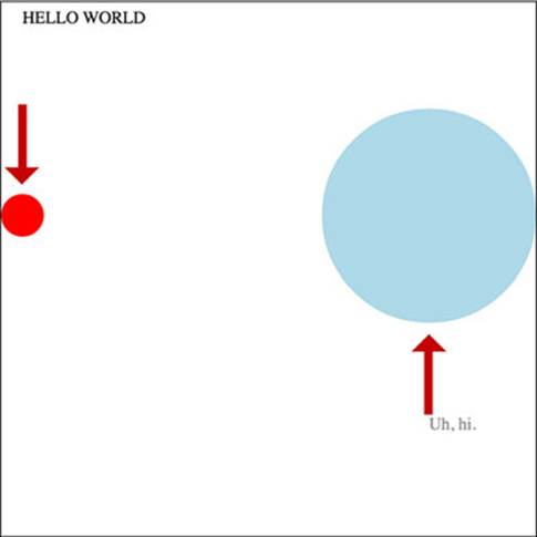
The .duration() method, as you can see, adjusts the setting over the course of the amount of time (again, in milliseconds) that you set it for.

That covers the basics of how D3 works and how it’s designed, and these fundamental concepts will surface again and again throughout the following chapters, where you’ll learn more complicated variations on representing and manipulating data.

1.7. Summary

In this chapter you’ve had an overview of D3 with a focus on how well suited it is for developers building web applications for the modern browser. I’ve highlighted the standardizations and advances that allow this to happen:

· A few examples of the kinds of data visualization you can create with D3

· A process map to show how to go from data to data visualization to interactivity, noting where you can find each step in this book

· An overview of the DOM, SVG, and CSS

· A first look at data-binding and selection to create and change elements on the page

· An overview of the different types of data you’ll encounter when planning and creating your data visualizations

· Some simple animations using D3 transitions

D3.js is another JavaScript library, one of thousands, but it’s also indicative of a change in our expectations of what a web page can do. Although you may initially use it to build one-off data visualizations, D3 has much more power and functionality than that. Throughout this book, we’ll explore the ways that you can use D3 to create rich, data-driven documents that will enthrall and impress.