Data Structures and Algorithms with JavaScript (2014)
Chapter 12. Sorting Algorithms
Two of the most common operations performed on data stored in a computer are sorting and searching. This has been true since the beginning of the computer industry, so this means that sorting and searching are two of the most studied operations in computer science. Many of the data structures discussed in this book are designed primarily to make sorting and/or searching the data stored in the data structure easier and more efficient.
This chapter will introduce you to some of the basic and advanced algorithms for sorting data. These algorithms depend only on the array as the means of storing data. In this chapter we’ll also look at ways of timing our programs to determine which algorithm is most efficient.
An Array Test Bed
We start this chapter by developing an array test bed to use in support of our study of basic sorting algorithms. We’ll build a class for array data and functions that encapsulates some of the normal array operations: inserting new data, displaying array data, and calling the different sorting algorithms. Included in the class is a swap() function we will use to exchange elements in the array.
Example 12-1 shows the code for this class.
Example 12-1. Array test bed class
function CArray(numElements) {
this.dataStore = [];
this.pos = 0;
this.numElements = numElements;
this.insert = insert;
this.toString = toString;
this.clear = clear;
this.setData = setData;
this.swap = swap;
for (var i = 0; i < numElements; ++i) {
this.dataStore[i] = i;
}
}
function setData() {
for (var i = 0; i < this.numElements; ++i) {
this.dataStore[i] = Math.floor(Math.random() *
(this.numElements+1));
}
}
function clear() {
for (var i = 0; i < this.dataStore.length; ++i) {
this.dataStore[i] = 0;
}
}
function insert(element) {
this.dataStore[this.pos++] = element;
}
function toString() {
var retstr = "";
for (var i = 0; i < this.dataStore.length; ++i) {
retstr += this.dataStore[i] + " ";
if (i > 0 && i % 10 == 0) {
retstr += "\n";
}
}
return retstr;
}
function swap(arr, index1, index2) {
var temp = arr[index1];
arr[index1] = arr[index2];
arr[index2] = temp;
}
Here is a simple program that uses the CArray class (the class is named CArray because JavaScript already has an Array class):
Example 12-2. Using the test bed class
var numElements = 100;
var myNums = new CArray(numElements);
myNums.setData();
print(myNums.toString());
The output from this program is:
76 69 64 4 64 73 47 34 65 93 32
59 4 92 84 55 30 52 64 38 74
40 68 71 25 84 5 57 7 6 40
45 69 34 73 87 63 15 96 91 96
88 24 58 78 18 97 22 48 6 45
68 65 40 50 31 80 7 39 72 84
72 22 66 84 14 58 11 42 7 72
87 39 79 18 18 9 84 18 45 50
43 90 87 62 65 97 97 21 96 39
7 79 68 35 39 89 43 86 5
Generating Random Data
You will notice that the setData() function generates random numbers to store in the array. The random() function, which is part of the Math class, generates random numbers in a range from 0 to 1, exclusive. In other words, no random number generated by the function will equal 0, and no random number will equal 1. These random numbers are not very useful, so we scale the numbers by multiplying the random number by the number of elements we want plus 1, and then use the floor() function from the Math class to finalize the number. As you can see from the preceding output, this formula succeeds in generating a set of random numbers between 1 and 100.
For more information on how JavaScript generates random numbers, see the Mozilla page, Using the Math.random() function, for random number generation.
Basic Sorting Algorithms
The fundamental concept of the basic sorting algorithms covered next is that there is a list of data that needs to be rearranged into sorted order. The technique used in these algorithms to rearrange data in a list is a set of nested for loops. The outer loop moves through the list item by item, while the inner loop is used to compare elements. These algorithms very closely simulate how humans sort data in real life, such as how a card player sorts cards when dealt a hand or how a teacher sorts papers in alphabetical or grade order.
Bubble Sort
The first sorting algorithm we will examine is the bubble sort. The bubble sort is one of the slowest sorting algorithms, but it is also one of the easiest sorts to implement.
The bubble sort gets its name because when data are sorted using the algorithm, values float like a bubble from one end of the array to the other. Assuming you are sorting a set of numbers into ascending order, larger values float to the right of the array and lower values float to the left. This behavior is the result of the algorithm moving through the array many times, comparing adjacent values, and swapping them if the value to the left is greater than the value to the right.
Here is a simple example of the bubble sort. We start with the following list:
E A D B H
The first pass of the sort yields the following list:
A E D B H
The first and second elements are swapped. The next pass of the sort leads to:
A D E B H
The second and third elements are swapped. The next pass leads to the following order:
A D B E H
as the third and fourth elements are swapped. And finally, the second and third elements are swapped again, leading to the final order:
A B D E H
Figure 12-1 illustrates how the bubble sort works with a larger data set of numbers. In the figure, we examine two particular values inserted into the array: 2 and 72. Each number is circled. You can watch how 72 moves from the beginning of the array to the middle of the array, and you can watch how 2 moves from just past the middle of the array to the beginning of the array.
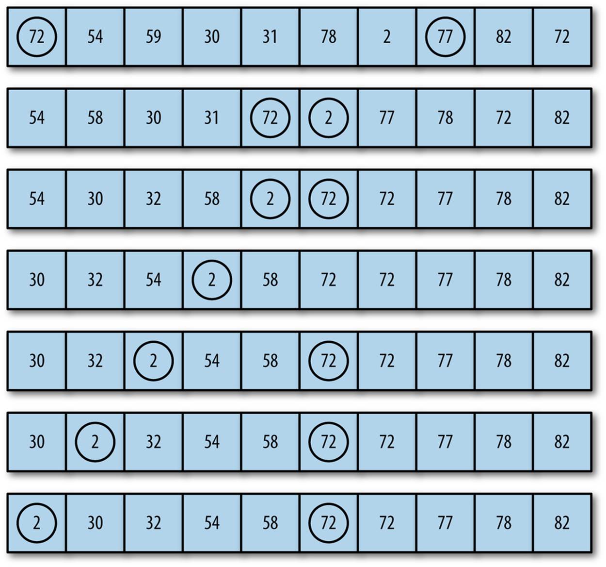
Figure 12-1. Bubble sort in action
Example 12-3 shows the code for the bubble sort:
Example 12-3. The bubbleSort() function
function bubbleSort() {
var numElements = this.dataStore.length;
var temp;
for (var outer = numElements; outer >= 2; --outer) {
for (var inner = 0; inner <= outer-1; ++inner) {
if (this.dataStore[inner] > this.dataStore[inner+1]) {
swap(this.dataStore, inner, inner+1);
}
}
}
}
Be sure to add a call to this function to the CArray constructor. Example 12-4 is a short program that sorts 10 numbers using the bubbleSort() function.
Example 12-4. Sorting 10 numbers with bubbleSort()
var numElements = 10;
var mynums = new CArray(numElements);
mynums.setData();
print(mynums.toString());
mynums.bubbleSort();
print();
print(mynums.toString());
The output from this program is:
10 8 3 2 2 4 9 5 4 3
2 2 3 3 4 4 5 8 9 10
We can see that the bubble sort algorithm works, but it would be nice to view the intermediate results of the algorithm, since a record of the sorting process is useful in helping us understand how the algorithm works. We can do that by the careful placement of the toString() function into the bubbleSort() function, which will display the current state of the array as the function proceeds (shown in Example 12-5).
Example 12-5. Adding a call to the toString() function to bubbleSort()
function bubbleSort() {
var numElements = this.dataStore.length;
var temp;
for (var outer = numElements; outer >= 2; --outer) {
for (var inner = 0; inner <= outer-1; ++inner) {
if (this.dataStore[inner] > this.dataStore[inner+1]) {
swap(this.dataStore, inner, inner+1);
}
}
print(this.toString());
}
}
When we rerun the preceding program with the toString() function included, we get the following output:
1 0 3 3 5 4 5 0 6 7
0 1 3 3 4 5 0 5 6 7
0 1 3 3 4 0 5 5 6 7
0 1 3 3 0 4 5 5 6 7
0 1 3 0 3 4 5 5 6 7
0 1 0 3 3 4 5 5 6 7
0 0 1 3 3 4 5 5 6 7
0 0 1 3 3 4 5 5 6 7
0 0 1 3 3 4 5 5 6 7
0 0 1 3 3 4 5 5 6 7
0 0 1 3 3 4 5 5 6 7
With this output, you can more easily see how the lower values work their way to the beginning of the array and how the higher values work their way to the end of the array.
Selection Sort
The next sorting algorithm we examine is the selection sort. This sort works by starting at the beginning of the array and comparing the first element with the remaining elements. After examining all the elements, the smallest element is placed in the first position of the array, and the algorithm moves to the second position. This process continues until the algorithm arrives at the next to last position in the array, at which point all the data is sorted.
Nested loops are used in the selection sort algorithm. The outer loop moves from the first element in the array to the next to last element; the inner loop moves from the second array element to the last element, looking for values that are smaller than the element currently being pointed to by the outer loop. After each iteration of the inner loop, the smallest value in the array is assigned its proper place in the array. Figure 12-2 illustrates how the selection sort algorithm works.
Here is a simple example of how selection sort works on a list of five items. The original list is:
E A D H B
The first pass looks for the minimal value and swaps it with the value at the front of the list:
A E D H B
The next pass finds the minimal value after the first element (which is now in place) and swaps it:
A B D H E
The D is in place so the next step swaps the E and the H, leading to the list being in order:
A B D E H
Figure 12-2 shows how selection sort works on a larger data set of numbers.
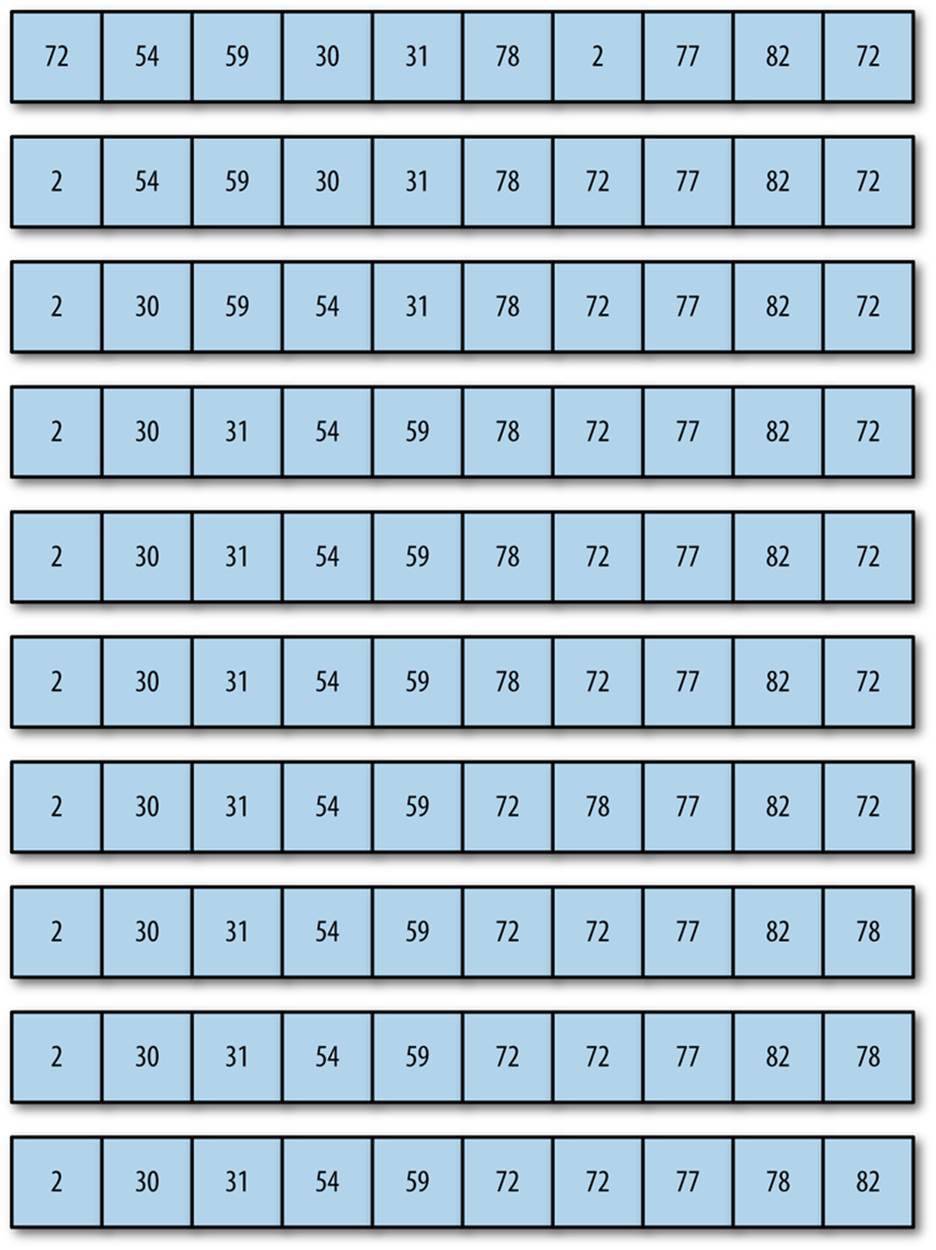
Figure 12-2. The selection sort algorithm
Example 12-6 shows the code for the selectionSort() function.
Example 12-6. The selectionSort() function
function selectionSort() {
var min, temp;
for (var outer = 0; outer <= this.dataStore.length-2; ++outer) {
min = outer;
for (var inner = outer + 1;
inner <= this.dataStore.length-1; ++inner) {
if (this.dataStore[inner] < this.dataStore[min]) {
min = inner;
}
}
swap(this.dataStore, outer, min);
}
}
Below is the output from one run of our program using the selectionSort() function. Add the following line right after the swap:
print(this.toString());
6 8 0 6 7 4 3 1 5 10
0 8 6 6 7 4 3 1 5 10
0 1 6 6 7 4 3 8 5 10
0 1 3 6 7 4 6 8 5 10
0 1 3 4 7 6 6 8 5 10
0 1 3 4 5 6 6 8 7 10
0 1 3 4 5 6 6 8 7 10
0 1 3 4 5 6 6 8 7 10
0 1 3 4 5 6 6 7 8 10
0 1 3 4 5 6 6 7 8 10
0 1 3 4 5 6 6 7 8 10
Insertion Sort
The insertion sort is analogous to the way humans sort data numerically or alphabetically. Let’s say I have asked each student in a class to turn in an index card with his or her name, student ID, and a short biographical sketch. The students return the cards in random order, but I want them alphabetized so I can compare them to my class roster easily.
I take the cards back to my office, clear off my desk, and pick the first card. The last name on the card is Smith. I place it at the top left corner of the desk and pick the second card. The last name on the card is Brown. I move Smith over to the right and put Brown in Smith’s place. The next card is Williams. It can be inserted at the far right of the desk without have to shift any of the other cards. The next card is Acklin. It has to go at the beginning of the list, so each of the other cards must be shifted one position to the right to make room for Acklin’s card. This is how the insertion sort works.
The insertion sort has two loops. The outer loop moves element by element through the array, while the inner loop compares the element chosen in the outer loop to the element next to it in the array. If the element selected by the outer loop is less than the element selected by the inner loop, array elements are shifted over to the right to make room for the inner-loop element, just as described in the previous name card example.
Example 12-7 shows the code for the insertion sort.
Example 12-7. The insertionSort() function
function insertionSort() {
var temp, inner;
for (var outer = 1; outer <= this.dataStore.length-1; ++outer) {
temp = this.dataStore[outer];
inner = outer;
while (inner > 0 && (this.dataStore[inner-1] >= temp)) {
this.dataStore[inner] = this.dataStore[inner-1];
--inner;
}
this.dataStore[inner] = temp;
}
}
Now let’s look at how the insertion sort works by running our program with a data set:
6 10 0 6 5 8 7 4 2 7
0 6 10 6 5 8 7 4 2 7
0 6 6 10 5 8 7 4 2 7
0 5 6 6 10 8 7 4 2 7
0 5 6 6 8 10 7 4 2 7
0 5 6 6 7 8 10 4 2 7
0 4 5 6 6 7 8 10 2 7
0 2 4 5 6 6 7 8 10 7
0 2 4 5 6 6 7 7 8 10
0 2 4 5 6 6 7 7 8 10
This output clearly shows that the insertion sort works not by making data exchanges, but by moving larger array elements to the right to make room for the smaller elements on the left side of the array.
Timing Comparisons of the Basic Sorting Algorithms
These three sorting algorithms are very similar in complexity, and theoretically, they should perform similarly. To determine the differences in performance among these three algorithms, we can use an informal timing system to compare how long it takes them to sort data sets. Being able to time these algorithms is important because, while you won’t see much of a difference in times of the sorting algorithms when you’re sorting 100 elements or even 1,000 elements, there can be a huge difference in the times these algorithms take to sort millions of elements.
The timing system we will use in this section is based on retrieving the system time using the JavaScript Date object’s getTime() function. Here is how the function works:
var start = new Date().getTime();
The getTime() function returns the system time in milliseconds. The following code fragment:
var start = new Date().getTime();
print(start);
results in the following output:
135154872720
To record the time it takes code to execute, we start the timer, run the code, and then stop the timer when the code is finished running. The time it takes to sort data is the difference between the recorded stopping time and the recorded starting time. Example 12-8 shows an example of timing afor loop that displays the numbers 1 through 100.
Example 12-8. Timing a for loop
var start = new Date().getTime();
for (var i = 1; i < 100; ++i) {
print(i);
}
var stop = new Date().getTime();
var elapsed = stop - start;
print("The elapsed time was: " + elapsed +
" milliseconds.");
The output, not including the starting and stopping time values, from the program is:
The elapsed time was: 91 milliseconds.
Now that we have a tool for measuring the efficiency of these sorting algorithms, let’s run some tests to compare them.
For our comparison of the three basic sorting algorithms, we will time the three algorithms sorting arrays with data set sizes of 100, 1,000, and 10,000. We expect not to see much difference among the algorithms for data set sizes of 100 and 1,000, but we do expect there to be some difference when using a data set size of 10,000.
Let’s start with an array of 100 randomly chosen integers. We also add a function for creating a new data set for each algorithm. Example 12-9 shows the code for this new function.
Example 12-9. Timing the sorting functions with 100 array elements
var numElements = 100;
var nums = new CArray(numElements);
nums.setData();
var start = new Date().getTime();
nums.bubbleSort();
var stop = new Date().getTime();
var elapsed = stop - start;
print("Elapsed time for the bubble sort on " +
numElements + " elements is: " + elapsed + " milliseconds.");
start = new Date().getTime();
nums.selectionSort();
stop = new Date().getTime();
elapsed = stop - start;
print("Elapsed time for the selection sort on " +
numElements + " elements is: " + elapsed + " milliseconds.");
start = new Date().getTime();
nums.insertionSort();
stop = new Date().getTime();
elapsed = stop - start;
print("Elapsed time for the insertion sort on " +
numElements + " elements is: " + elapsed + " milliseconds.");
Here are the results (note that I ran these tests on an Intel 2.4 GHz processor):
Elapsed time for the bubble sort on 100 elements is: 0 milliseconds.
Elapsed time for the selection sort on 100 elements is: 1 milliseconds.
Elapsed time for the insertion sort on 100 elements is: 0 milliseconds.
Clearly, there is not any significant difference among the three algorithms.
For the next test, we change the numElements variable to 1,000. Here are the results:
Elapsed time for the bubble sort on 1000 elements is: 12 milliseconds.
Elapsed time for the selection sort on 1000 elements is: 7 milliseconds.
Elapsed time for the insertion sort on 1000 elements is: 6 milliseconds.
For 1,000 numbers, the selection sort and the insertion sort are almost twice as fast as the bubble sort.
Finally, we test the algorithms with 10,000 numbers:
Elapsed time for the bubble sort on 10000 elements is: 1096 milliseconds.
Elapsed time for the selection sort on 10000 elements is: 591 milliseconds.
Elapsed time for the insertion sort on 10000 elements is: 471 milliseconds.
The results for 10,000 numbers are consistent with the results for 1,000 numbers. Selection sort and insertion sort are faster than the bubble sort, and the insertion sort is the fastest of the three sorting algorithms. Keep in mind, however, that these tests must be run several times for the results to be considered statistically valid.
Advanced Sorting Algorithms
In this section we will cover more advanced algorithms for sorting data. These sorting algorithms are generally considered the most efficient for large data sets, where data sets can have millions of elements rather than just hundreds or even thousands. The algorithms we study in this chapter include Quicksort, Shellsort, Mergesort, and Heapsort. We discuss each algorithm’s implementation and then compare their efficiency by running timing tests.
The Shellsort Algorithm
The first advanced sorting algorithm we’ll examine is the Shellsort algorithm. Shellsort is named after its inventor, Donald Shell. This algorithm is based on the insertion sort but is a big improvement over that basic sorting algorithm. Shellsort’s key concept is that it compares distant elements first, rather than adjacent elements, as is done in the insertion sort. Elements that are far out of place can be put into place more efficiently using this scheme than by simply comparing neighboring elements. As the algorithm loops through the data set, the distance between each element decreases until, when at the end of the data set, the algorithm is comparing elements that are adjacent.
Shellsort works by defining a gap sequence that indicates how far apart compared elements are when starting the sorting process. The gap sequence can be defined dynamically, but for most practical applications, you can predefine the gap sequence the algorithm will use. There are several published gap sequences that produce different results. We are going to use the sequence defined by Marcin Ciura in his paper on best increments for average case of Shellsort (“Best Increments for the Average Case of Shell Sort”, 2001). The gap sequence is: 701, 301, 132, 57, 23, 10, 4, 1. However, before we write code for the average case, we are going to examine how the algorithm works with a small data set.
Figure 12-3 demonstrates how the gap sequence works with the Shellsort algorithm.
Let’s start with a look at the code for the Shellsort algorithm:
function shellsort() {
for (var g = 0; g < this.gaps.length; ++g) {
for (var i = this.gaps[g]; i < this.dataStore.length; ++i) {
var temp = this.dataStore[i];
for (var j = i; j >= this.gaps[g] &&
this.dataStore[j-this.gaps[g]] > temp;
j -= this.gaps[g]) {
this.dataStore[j] = this.dataStore[j - this.gaps[g]];
}
this.dataStore[j] = temp;
}
}
}
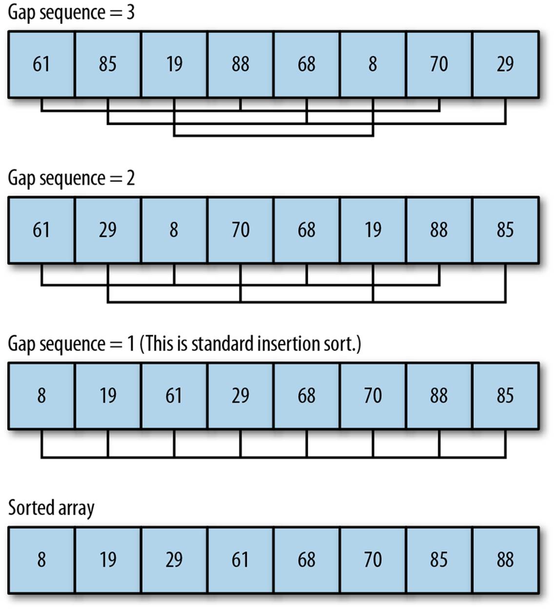
Figure 12-3. The Shellsort algorithm with an initial gap sequence of 3
For this program to work with our CArray class test bed, we need to add a definition of the gap sequence to the class definition. Add the following code into the constructor function for CArray:
this.gaps = [5,3,1];
And add this function to the code:
function setGaps(arr) {
this.gaps = arr;
}
Finally, add a reference to the shellsort() function to the CArray class constructor as well as the shellsort() code itself.
The outer loop controls the movement within the gap sequence. In other words, for the first pass through the data set, the algorithm is going to examine elements that are five elements away from each other. The next pass will examine elements that are three elements away from each other. The last pass performs a standard insertion sort on element that are one place away, which means they are adjacent. By the time this last pass begins, many of the elements will already be in place, and the algorithm won’t have to exchange many elements. This is where the algorithm gains efficiency over insertion sort. Figure 12-3 illustrates how the Shellsort algorithm works on a data set of 10 random numbers with a gap sequence of 5, 3, 1.
Now let’s put the algorithm to work on a real example. We add a print() statement to shellsort() so that we can follow the progress of the algorithm while it sorts the data set. Each gap pass is noted, followed by the order of the data set after sorting with that particular gap. The program is shown in Example 12-10.
Example 12-10. Running shellsort() on a small data set
load("CArray.js")
var nums = new CArray(10);
nums.setData();
print("Before Shellsort: \n");
print(nums.toString());
print("\nDuring Shellsort: \n");
nums.shellsort();
print("\nAfter Shellsort: \n");
print(nums.toString());
The output from this program is:
Before Shellsort:
6 0 2 9 3 5 8 0 5 4
During Shellsort:
5 0 0 5 3 6 8 2 9 4 // gap 5
4 0 0 5 2 6 5 3 9 8 // gap 3
0 0 2 3 4 5 5 6 8 9 // gap 1
After Shellsort:
0 0 2 3 4 5 5 6 8 9
To understand how Shellsort works, compare the initial state of the array with its state after the gap sequence of 5 was sorted. The first element of the initial array, 6, was swapped with the fifth element after it, 5, because 5 < 6.
Now compare the gap 5 line with the gap 3 line. The 3 in the gap 5 line is swapped with the 2 because 2 < 3 and 2 is the third element after the 3. By simply counting the current gap sequence number down from the current element in the loop, and comparing the two numbers, you can trace any run of the Shellsort algorithm.
Having now seen some details of how the Shellsort algorithm works, let’s use a larger gap sequence and run it with a larger data set (100 elements). Here is the output:
Before Shellsort:
19 19 54 60 66 69 45 40 36 90 22
93 23 0 88 21 70 4 46 30 69
75 41 67 93 57 94 21 75 39 50
17 8 10 43 89 1 0 27 53 43
51 86 39 86 54 9 49 73 62 56
84 2 55 60 93 63 28 10 87 95
59 48 47 52 91 31 74 2 59 1
35 83 6 49 48 30 85 18 91 73
90 89 1 22 53 92 84 81 22 91
34 61 83 70 36 99 80 71 1
After Shellsort:
0 0 1 1 1 1 2 2 4 6 8
9 10 10 17 18 19 19 21 21 22
22 22 23 27 28 30 30 31 34 35
36 36 39 39 40 41 43 43 45 46
47 48 48 49 49 50 51 52 53 53
54 54 55 56 57 59 59 60 60 61
62 63 66 67 69 69 70 70 71 73
73 74 75 75 80 81 83 83 84 84
85 86 86 87 88 89 89 90 90 91
91 91 92 93 93 93 94 95 99
We will revisit the shellsort() algorithm again when we compare it to other advanced sorting algorithms later in the chapter.
Computing a dynamic gap sequence
Robert Sedgewick, coauthor of Algorithms, 4E (Addison-Wesley), defines a shellsort() function that uses a formula to dynamically compute the gap sequence to use with Shellsort. Sedgewick’s algorithm determines the initial gap value using the following code fragment:
var N = this.dataStore.length;
var h = 1;
while (h < N/3) {
h = 3 * h + 1;
}
Once the gap value is determined, the function works like our previous shellsort() function, except the last statement before going back into the outer loop computes a new gap value:
h = (h-1)/3;
Example 12-11 provides the complete definition of this new shellsort() function, along with a swap() function it uses, and a program to test the function definition.
Example 12-11. shellsort() with a dynamically computed gap sequence
function shellsort1() {
var N = this.dataStore.length;
var h = 1;
while (h < N/3) {
h = 3 * h + 1;
}
while (h >= 1) {
for (var i = h; i < N; i++) {
for (var j = i; j >= h && this.dataStore[j] < this.dataStore[j-h];
j -= h) {
swap(this.dataStore, j, j-h);
}
}
h = (h-1)/3;
}
}
load("CArray.js")
var nums = new CArray(100);
nums.setData();
print("Before Shellsort1: \n");
print(nums.toString());
nums.shellsort1();
print("\nAfter Shellsort1: \n");
print(nums.toString());
The output from this program is:
Before Shellsort1:
92 31 5 96 44 88 34 57 44 72 20
83 73 8 42 82 97 35 60 9 26
14 77 51 21 57 54 16 97 100 55
24 86 70 38 91 54 82 76 78 35
22 11 34 13 37 16 48 83 61 2
5 1 6 85 100 16 43 74 21 96
44 90 55 78 33 55 12 52 88 13
64 69 85 83 73 43 63 1 90 86
29 96 39 63 41 99 26 94 19 12
84 86 34 8 100 87 93 81 31
After Shellsort1:
1 1 2 5 5 6 8 8 9 11 12
12 13 13 14 16 16 16 19 20 21
21 22 24 26 26 29 31 31 33 34
34 34 35 35 37 38 39 41 42 43
43 44 44 44 48 51 52 54 54 55
55 55 57 57 60 61 63 63 64 69
70 72 73 73 74 76 77 78 78 81
82 82 83 83 83 84 85 85 86 86
86 87 88 88 90 90 91 92 93 94
96 96 96 97 97 99 100 100 100
Before we leave the Shellsort algorithm, we need to compare the efficiency of our two shellsort() functions. A program that compares running times of the two functions is shown in Example 12-12. Both algorithms use Ciura’s sequence for the gap sequence.
Example 12-12. Comparing shellsort() algorithms
load("CArray.js");
var nums = new CArray(10000);
nums.setData();
var start = new Date().getTime();
nums.shellsort();
var stop = new Date().getTime();
var elapsed = stop - start;
print("Shellsort with hard-coded gap sequence: " + elapsed + " ms.");
nums.clear();
nums.setData();
start = new Date().getTime();
nums.shellsort1();
stop = new Date().getTime();
print("Shellsort with dynamic gap sequence: " + elapsed + " ms.");
The results from this program are:
Shellsort with hard-coded gap sequence: 3 ms.
Shellsort with dynamic gap sequence: 3 ms.
Both algorithms sorted the data in the same amount of time. Here is the output from running the program with 100,000 data elements:
Shellsort with hard-coded gap sequence: 43 ms.
Shellsort with dynamic gap sequence: 43 ms.
Clearly, both of these algorithms sort data with the same efficiency, so you can use either of them with confidence.
The Mergesort Algorithm
The Mergesort algorithm is so named because it works by merging sorted sublists together to form a larger, completely sorted list. In theory, this algorithm should be easy to implement. We need two sorted subarrays and a third array into which we merge the two subarrays by comparing data elements and inserting the smallest element value. In practice, however, Mergesort has some problems because if we are trying to sort a very large data set using the algorithm, the amount of space we need to store the two merged subarrays can be quite large. Since space is not such an issue in these days of inexpensive memory, it is worth implementing Mergesort to see how it compares in efficiency to other sorting algorithms.
Top-down Mergesort
It is customary, though not necessary, to implement Mergesort as a recursive algorithm. However, it is not possible to do so in JavaScript, as the recursion goes too deep for the language to handle. Instead, we will implement the algorithm in a nonrecursive way, using a strategy called bottom-up Mergesort.
Bottom-up Mergesort
The nonrecursive, or iterative, version of Mergesort is referred to as a bottom-up process. The algorithm begins by breaking down the data set being sorted into a set of one-element arrays. Then these arrays are slowly merged by creating a set of left and right subarrays, each holding the partially sorted data until all that is left is one array with the data perfectly sorted. Figure 12-4 illustrates how the bottom-up Mergesort algorithm works.
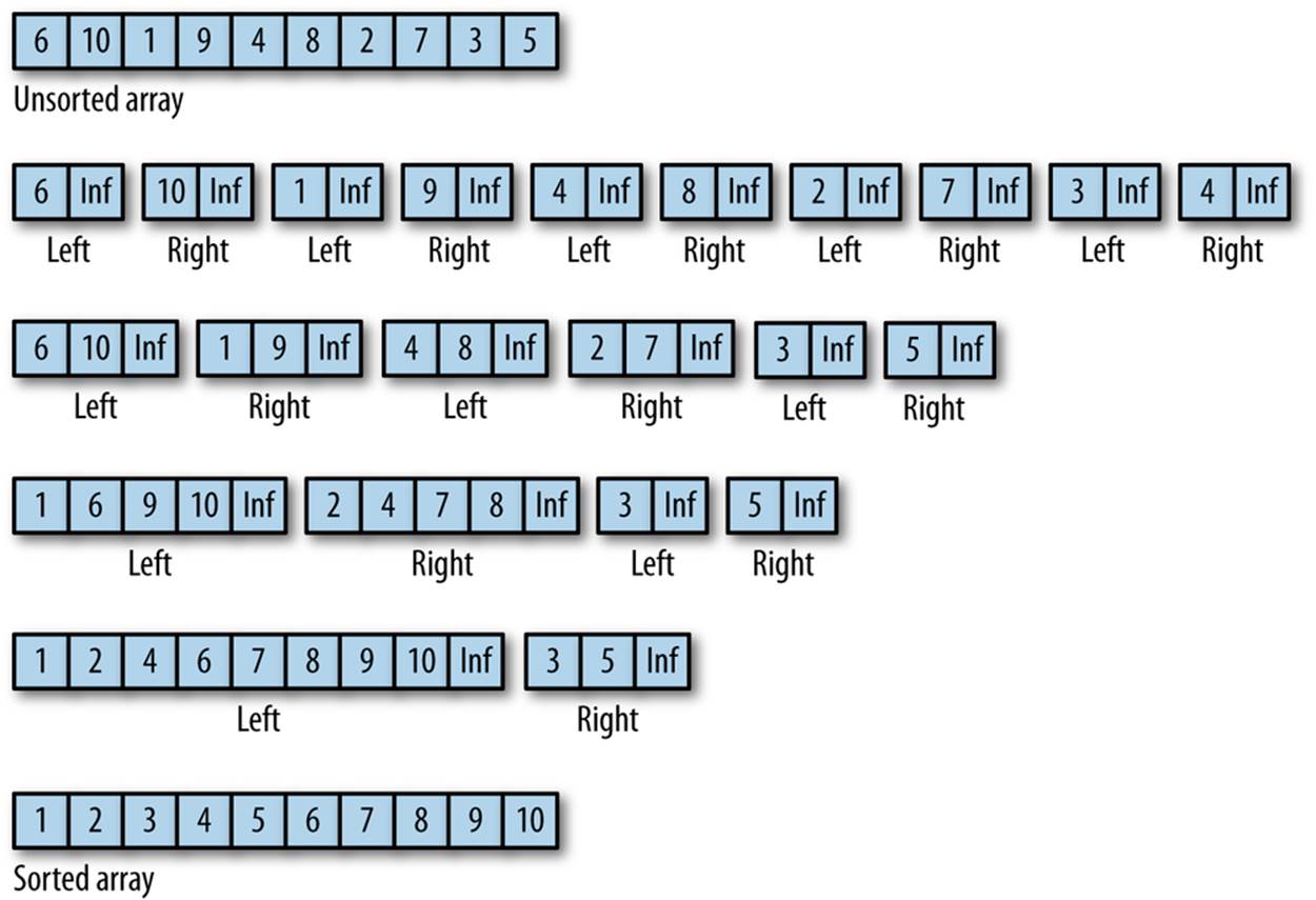
Figure 12-4. The bottom-up Mergesort algorithm
Before we show you the JavaScript code for Mergesort, here is the output from a JavaScript program that uses bottom-up Mergesort to sort an array of 10 integers:
6,10,1,9,4,8,2,7,3,5
left array - 6,Infinity
right array - 10,Infinity
left array - 1,Infinity
right array - 9,Infinity
left array - 4,Infinity
right array - 8,Infinity
left array - 2,Infinity
right array - 7,Infinity
left array - 3,Infinity
right array - 5,Infinity
left array - 6,10,Infinity
right array - 1,9,Infinity
left array - 4,8,Infinity
right array - 2,7,Infinity
left array - 1,6,9,10,Infinity
right array - 2,4,7,8,Infinity
left array - 1,2,4,6,7,8,9,10,Infinity
right array - 3,5,Infinity
1,2,3,4,5,6,7,8,9,10
The value Infinity is used as a sentinel value to indicate the end of either the left or right subarray.
Each array element starts out in its own left or right array. Then the two arrays are merged, first into two elements each, then into four elements each, except for 3 and 5, which stay apart until the last iteration, when they are combined into the right array and then merged into the left array to re-form the original array.
Now that we have seen how the bottom-up Mergesort works, Example 12-13 presents the code that created the preceding output.
Example 12-13. A bottom-up Mergesort JavaScript implementation
function mergeSort(arr) {
if (arr.length < 2) {
return;
}
var step = 1;
var left, right;
while (step < arr.length) {
left = 0;
right = step;
while (right + step <= arr.length) {
mergeArrays(arr, left, left+step, right, right+step);
left = right + step;
right = left + step;
}
if (right < arr.length) {
mergeArrays(arr, left, left+step, right, arr.length);
}
step *= 2;
}
}
function mergeArrays(arr, startLeft, stopLeft, startRight, stopRight) {
var rightArr = new Array(stopRight - startRight + 1);
var leftArr = new Array(stopLeft - startLeft + 1);
k = startRight;
for (var i = 0; i < (rightArr.length-1); ++i) {
rightArr[i] = arr[k];
++k;
}
k = startLeft;
for (var i = 0; i < (leftArr.length-1); ++i) {
leftArr[i] = arr[k];
++k;
}
rightArr[rightArr.length-1] = Infinity; // a sentinel value
leftArr[leftArr.length-1] = Infinity; // a sentinel value
var m = 0;
var n = 0;
for (var k = startLeft; k < stopRight; ++k) {
if (leftArr[m] <= rightArr[n]) {
arr[k] = leftArr[m];
m++;
}
else {
arr[k] = rightArr[n];
n++;
}
}
print("left array - ", leftArr);
print("right array - ", rightArr);
}
var nums = [6,10,1,9,4,8,2,7,3,5];
print(nums);
print();
mergeSort(nums);
print();
print(nums);
The key feature of the mergeSort() function is the step variable, which is used to control the size of the leftArr and rightArr subarrays found in the mergeArrays() function. By controlling the size of the subarrays, the sort process is relatively efficient, since it doesn’t take much time to sort a small array. This makes merging efficient also, since it is much easier to merge data into sorted order when the unmerged data is already sorted.
Our next step with Mergesort is to add it to the CArray class and time it on a larger data set. Example 12-14 shows the CArray class with the mergeSort() and mergeArrays() functions added to its definition.
Example 12-14. Mergesort added to the CArray class
function CArray(numElements) {
this.dataStore = [];
this.pos = 0;
this.gaps = [5,3,1];
this.numElements = numElements;
this.insert = insert;
this.toString = toString;
this.clear = clear;
this.setData = setData;
this.setGaps = setGaps;
this.shellsort = shellsort;
this.mergeSort = mergeSort;
this.mergeArrays = mergeArrays;
for (var i = 0; i < numElements; ++i) {
this.dataStore[i] = 0;
}
}
// other function definitions go here
function mergeArrays(arr,startLeft, stopLeft, startRight, stopRight) {
var rightArr = new Array(stopRight - startRight + 1);
var leftArr = new Array(stopLeft - startLeft + 1);
k = startRight;
for (var i = 0; i < (rightArr.length-1); ++i) {
rightArr[i] = arr[k];
++k;
}
k = startLeft;
for (var i = 0; i < (leftArr.length-1); ++i) {
leftArr[i] = arr[k];
++k;
}
rightArr[rightArr.length-1] = Infinity; // a sentinel value
leftArr[leftArr.length-1] = Infinity; // a sentinel value
var m = 0;
var n = 0;
for (var k = startLeft; k < stopRight; ++k) {
if (leftArr[m] <= rightArr[n]) {
arr[k] = leftArr[m];
m++;
}
else {
arr[k] = rightArr[n];
n++;
}
}
print("left array - ", leftArr);
print("right array - ", rightArr);
}
function mergeSort() {
if (this.dataStore.length < 2) {
return;
}
var step = 1;
var left, right;
while (step < this.dataStore.length) {
left = 0;
right = step;
while (right + step <= this.dataStore.length) {
mergeArrays(this.dataStore, left, left+step, right, right+step);
left = right + step;
right = left + step;
}
if (right < this.dataStore.length) {
mergeArrays(this.dataStore, left, left+step, right, this.dataStore.length);
}
step *= 2;
}
}
var nums = new CArray(10);
nums.setData();
print(nums.toString());
nums.mergeSort();
print(nums.toString());
The Quicksort Algorithm
The Quicksort algorithm is one of the fastest sorting algorithms for large data sets. Quicksort is a divide-and-conquer algorithm that recursively breaks a list of data into successively smaller sublists consisting of the smaller elements and the larger elements. The algorithm continues this process until all the data in the list is sorted.
The algorithm divides the list into sublists by selecting one element of the list as a pivot. Data is sorted around the pivot by moving elements less than the pivot to the bottom of the list and elements that are greater than the pivot to the top of the list.
Figure 12-5 demonstrates how data is sorted around a pivot.
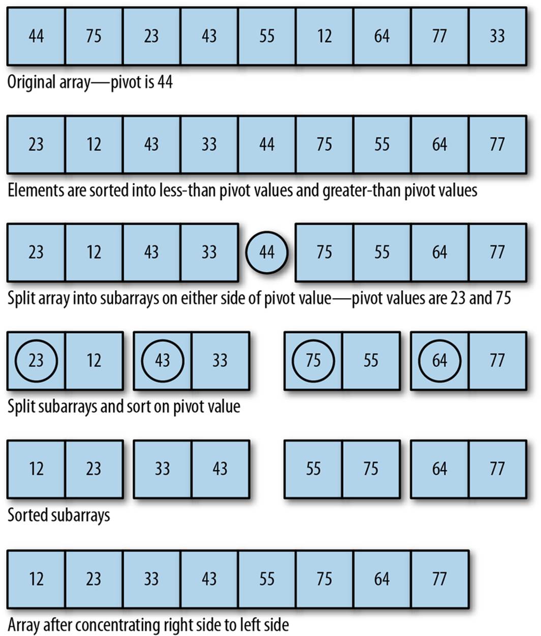
Figure 12-5. Sorting data around a pivot
Algorithm and pseudocode for the Quicksort algorithm
The algorithm for Quicksort is:
1. Pick a pivot element that divides the list into two sublists.
2. Reorder the list so that all elements less than the pivot element are placed before the pivot and all elements greater than the pivot are placed after it.
3. Repeat steps 1 and 2 on both the list with smaller elements and the list of larger elements.
This algorithm then translates into the following JavaScript program:
function qSort(list) {
if (list.length == 0) {
return [];
}
var lesser = [];
var greater = [];
var pivot = list[0];
for (var i = 1; i < list.length; i++) {
if (list[i] < pivot) {
lesser.push(list[i]);
} else {
greater.push(list[i]);
}
}
return qSort(lesser).concat(pivot, qSort(greater));
}
The function first tests to see if the array has a length of 0. If so, then the array doesn’t need sorting and the function returns. Otherwise, two arrays are created, one to hold the elements lesser than the pivot and the other to hold the elements greater than the pivot. The pivot is then selected by selecting the first element of the array. Next, the function loops over the array elements and places them in their proper array based on their value relative to the pivot value. The function is then called recursively on both the lesser array and the greater array. When the recursion is complete, the greater array is concatenated to the lesser array to form the sorted array and is returned from the function.
Let’s test the algorithm with some data. Because our qSort program uses recursion, we won’t use the array test bed; instead, we’ll just create an array of random numbers and sort the array directly. The program is shown in Example 12-15.
Example 12-15. Sorting data with Quicksort
function qSort(arr)
{
if (arr.length == 0) {
return [];
}
var left = [];
var right = [];
var pivot = arr[0];
for (var i = 1; i < arr.length; i++) {
if (arr[i] < pivot) {
left.push(arr[i]);
} else {
right.push(arr[i]);
}
}
return qSort(left).concat(pivot, qSort(right));
}
var a = [];
for (var i = 0; i < 10; ++i) {
a[i] = Math.floor((Math.random()*100)+1);
}
print(a);
print();
print(qSort(a));
The output from this program is:
68,80,12,80,95,70,79,27,88,93
12,27,68,70,79,80,80,88,93,95
The Quicksort algorithm is best to use on large data sets; its performance degrades for smaller data sets.
To better demonstrate how Quicksort works, this next program highlights the pivot as it is chosen and how data is sorted around the pivot:
function qSort(arr)
{
if (arr.length == 0) {
return [];
}
var left = [];
var right = [];
var pivot = arr[0];
for (var i = 1; i < arr.length; i++) {
print("pivot: " + pivot + " current element: " + arr[i]);
if (arr[i] < pivot) {
print("moving " + arr[i] + " to the left");
left.push(arr[i]);
} else {
print("moving " + arr[i] + " to the right");
right.push(arr[i]);
}
}
return qSort(left).concat(pivot, qSort(right));
}
var a = [];
for (var i = 0; i < 10; ++i) {
a[i] = Math.floor((Math.random()*100)+1);
}
print(a);
print();
print(qSort(a));
The output from this program is:
9,3,93,9,65,94,50,90,12,65
pivot: 9 current element: 3
moving 3 to the left
pivot: 9 current element: 93
moving 93 to the right
pivot: 9 current element: 9
moving 9 to the right
pivot: 9 current element: 65
moving 65 to the right
pivot: 9 current element: 94
moving 94 to the right
pivot: 9 current element: 50
moving 50 to the right
pivot: 9 current element: 90
moving 90 to the right
pivot: 9 current element: 12
moving 12 to the right
pivot: 9 current element: 65
moving 65 to the right
pivot: 93 current element: 9
moving 9 to the left
pivot: 93 current element: 65
moving 65 to the left
pivot: 93 current element: 94
moving 94 to the right
pivot: 93 current element: 50
moving 50 to the left
pivot: 93 current element: 90
moving 90 to the left
pivot: 93 current element: 12
moving 12 to the left
pivot: 93 current element: 65
moving 65 to the left
pivot: 9 current element: 65
moving 65 to the right
pivot: 9 current element: 50
moving 50 to the right
pivot: 9 current element: 90
moving 90 to the right
pivot: 9 current element: 12
moving 12 to the right
pivot: 9 current element: 65
moving 65 to the right
pivot: 65 current element: 50
moving 50 to the left
pivot: 65 current element: 90
moving 90 to the right
pivot: 65 current element: 12
moving 12 to the left
pivot: 65 current element: 65
moving 65 to the right
pivot: 50 current element: 12
moving 12 to the left
pivot: 90 current element: 65
moving 65 to the left
3,9,9,12,50,65,65,90,93,94
Exercises
1. Run the three algorithms discussed in this chapter with string data rather than numeric data and compare the running times for the different algorithms. Are the results consistent with the results of using numeric data?
2. Create an array of 1,000 integers already sorted into numeric order. Write a program that runs each sorting algorithm with this array, timing each algorithm and comparing the times. How do these times compare to the times for sorting an array in random order?
3. Create an array of 1,000 integers sorted in reverse numerical order. Write a program that runs each sorting algorithm with this array, timing each algorithm, and compare the times.
4. Create an array of over 10,000 randomly generated integers and sort the array using both Quicksort and the JavaScript built-in sorting function, timing each function. Is there a time difference between the two functions?
All materials on the site are licensed Creative Commons Attribution-Sharealike 3.0 Unported CC BY-SA 3.0 & GNU Free Documentation License (GFDL)
If you are the copyright holder of any material contained on our site and intend to remove it, please contact our site administrator for approval.
© 2016-2026 All site design rights belong to S.Y.A.