Data Structures and Algorithms with JavaScript (2014)
Chapter 13. Searching Algorithms
Searching for data is a fundamental computer programming task that has been studied for many years. This chapter looks at just one aspect of the search problem—searching for a specified value in a list.
There are two ways to search for data in a list: sequential search and binary search. A sequential search is used when the items in a list are in random order; a binary search is used when the items in a list are in sorted order. Binary search is the more efficient algorithm, but you also have to take into account the extra time it takes to sort the data set before being able to search it for a value.
Sequential Search
The most obvious way to search for data in a list is to begin at the first element and move to each element in the list until you either find the data you are looking for or you reach the end of the list. This is called a sequential search, sometimes also called a linear search. It is an example of abrute-force search technique, where potentially every element in the data structure is visited on the way to a solution.
A sequential search is very easy to implement. Simply start a loop at the beginning of the list and compare each element to the data you are searching for. If you find a match, the search is over. If you get to the end of the list without generating a match, then the data searched for is not in the list.
Example 13-1 shows a function for performing sequential search on an array.
Example 13-1. The seqSearch() function
function seqSearch(arr, data) {
for (var i = 0; i < arr.length; ++i) {
if (arr[i] == data) {
return true;
}
}
return false;
}
If the data argument is found in the array, the function returns true immediately. If the function gets to the end of the array without finding a match, the function returns false.
Example 13-2 presents a program to test our sequential search function, including a function to make it easy to display the array’s contents. As in Chapter 12, we use random number generation to populate an array with random numbers in the range of 1 to 100. We also use a function to display the contents of the array, just as we did in Chapter 12.
Example 13-2. Executing the +seqSearch() function
function dispArr(arr) {
for (var i = 0; i < arr.length; ++i) {
putstr(arr[i] + " ");
if (i % 10 == 9) {
putstr("\n");
}
}
if (i % 10 != 0) {
putstr("\n");
}
}
var nums = [];
for (var i = 0; i < 100; ++i) {
nums[i] = Math.floor(Math.random() * 101);
}
dispArr(nums);
putstr("Enter a number to search for: ");
var num = parseInt(readline());
print();
if (seqSearch(nums, num)) {
print(num + " is in the array.");
}
else {
print(num + " is not in the array.");
}
print();
dispArr(nums);
This program creates an array with random numbers in the range of 0 to 100. The user enters a value, the value is searched for, and the result is displayed. Finally, the program displays the complete array as proof of the validity of the function’s return value. Here is a sample run of the program:
Enter a number to search for: 23
23 is in the array.
13 95 72 100 94 90 29 0 66 2 29
42 20 69 50 49 100 34 71 4 26
85 25 5 45 67 16 73 64 58 53
66 73 46 55 64 4 84 62 45 99
77 62 47 52 96 16 97 79 55 94
88 54 60 40 87 81 56 22 30 91
99 90 23 18 33 100 63 62 46 6
10 5 25 48 9 8 95 33 82 32
56 23 47 36 88 84 33 4 73 99
60 23 63 86 51 87 63 54 62
We can also write the sequential search function so that it returns the position where a match is found. Example 13-3 provides the definition of this new version of seqSearch().
Example 13-3. Modifying the seqSearch() function to return the position found (or -1)
function seqSearch(arr, data) {
for (var i = 0; i < arr.length; ++i) {
if (arr[i] == data) {
return i;
}
}
return -1;
}
Notice that if the element searched for is not found, the function returns -1. This is the best value to return for the function since an array element cannot be stored in position -1.
Example 13-4 presents a program that uses this second definition of seqSearch().
Example 13-4. Testing the modified seqSearch() function
var nums = [];
for (var i = 0; i < 100; ++i) {
nums[i] = Math.floor(Math.random() * 101);
}
putstr("Enter a number to search for: ");
var num = readline();
print();
var position = seqSearch(nums, num);
if (position > -1) {
print(num + " is in the array at position " + position);
}
else {
print(num + " is not in the array.");
}
print();
dispArr(nums);
Here is one run of the program:
Enter a number to search for: 22
22 is in the array at position 35
35 36 38 50 24 81 78 43 26 26 89
88 39 1 56 92 17 77 53 36 73
61 54 32 97 27 60 67 16 70 59
4 76 7 38 22 87 30 42 91 79
6 61 56 84 6 82 55 91 10 42
37 46 4 85 37 18 27 76 29 2
76 46 87 16 1 78 6 43 72 2
51 65 70 91 73 67 1 57 53 31
16 64 89 84 76 91 15 39 38 3
19 66 44 97 29 6 1 72 62
Keep in mind that the seqSearch() function is not as fast as the built-in Array.indexOf() function, but is shown here to demonstrate how search works.
Searching for Minimum and Maximum Values
Computer programming problems often involve searching for minimum and maximum values. In a sorted data structure, searching for these values is a trivial task. Searching an unsorted data structure, on the other hand, is a more challenging task.
Let’s start by determining how we should search an array for a minimum value. Here is one algorithm:
1. Assign the first element of the array to a variable as the minimum value.
2. Begin looping through the array, starting with the second element, comparing each element with the current minimum value.
3. If the current element has a lesser value than the current minimum value, assign the current element as the new minimum value.
4. Move to the next element and repeat step 3.
5. The minimum value is stored in the variable when the program ends.
The operation of this algorithm is demonstrated in Figure 13-1.
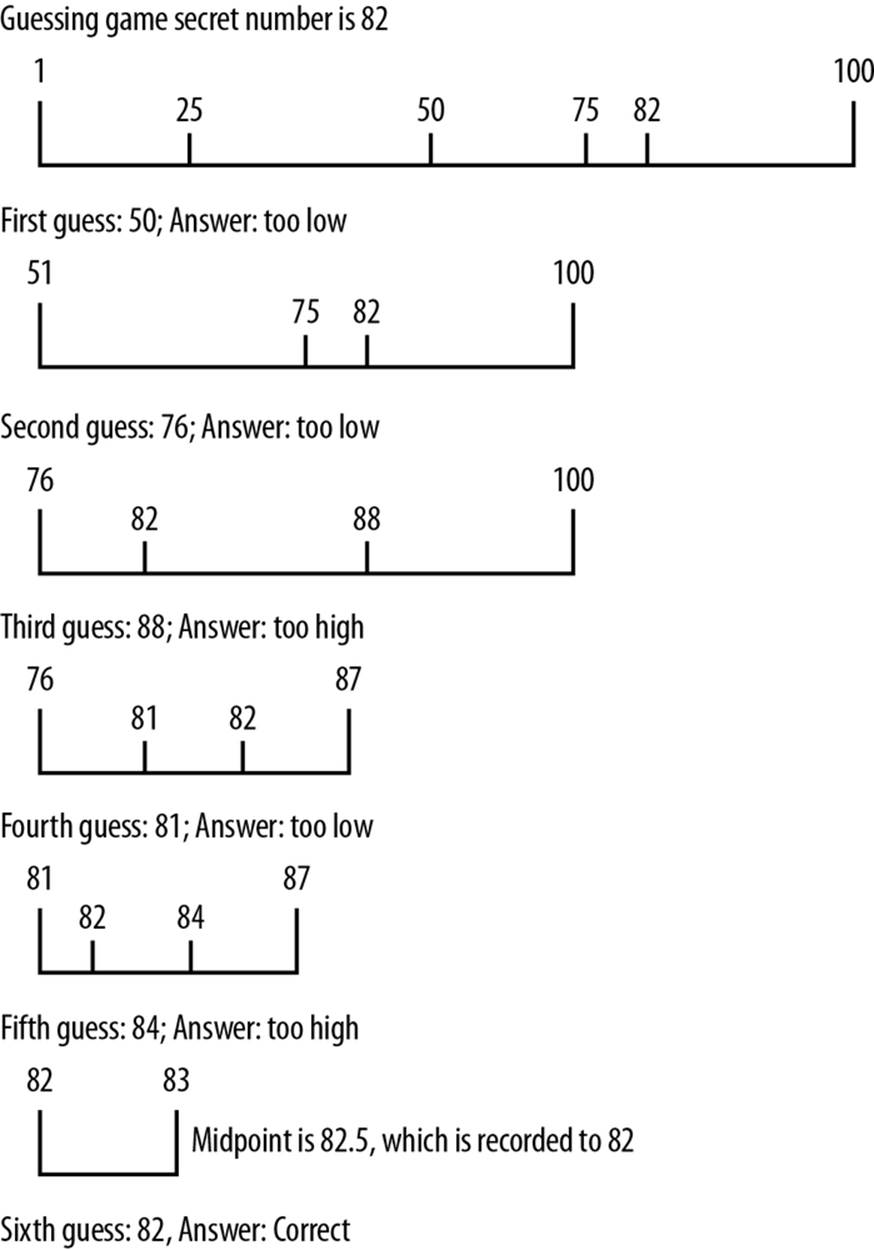
Figure 13-1. Searching for the minimum value of an array
This algorithm is easily transformed into a JavaScript function, as shown in Example 13-5.
Example 13-5. The findMin() function
function findMin(arr) {
var min = arr[0];
for (var i = 1; i < arr.length; ++i) {
if (arr[i] < min) {
min = arr[i];
}
}
return min;
}
The key thing to notice about this function is that it begins with the second array element, since we are assigning the first array element as the current minimum value.
Let’s test the function in a program, shown in Example 13-6.
Example 13-6. Finding the minimum value of an array
var nums = [];
for (var i = 0; i < 100; ++i) {
nums[i] = Math.floor(Math.random() * 101);
}
var minValue = findMin(nums);
dispArr(nums);
print();
print("The minimum value is: " + minValue);
Here is the output from running this program:
89 30 25 32 72 70 51 42 25 24 53
55 78 50 13 40 48 32 26 2 14
33 45 72 56 44 21 88 27 68 15
93 98 73 28 16 46 87 28 65 38
67 16 85 63 23 69 64 91 9 70
81 27 97 82 6 88 3 7 46 13
11 64 31 26 38 28 13 17 69 90
1 6 7 64 43 9 73 80 98 46
27 22 87 49 83 6 39 42 51 54
84 34 53 78 40 14 5 76 62
The minimum value is: 1
The algorithm for finding the maximum value works in a similar fashion. We assign the first element of the array as the maximum value and then loop through the rest of the array, comparing each element to the current maximum value. If the current element is greater than the current maximum value, that element’s value is stored in the variable. Example 13-7 shows the function definition.
Example 13-7. The findMax() function
function findMax(arr) {
var max = arr[0];
for (var i = 1; i < arr.length; ++i) {
if (arr[i] > max) {
max = arr[i];
}
}
return max;
}
Example 13-8 shows a program that finds both the minimum value and the maximum value of an array.
Example 13-8. Using the findMax() function
var nums = [];
for (var i = 0; i < 100; ++i) {
nums[i] = Math.floor(Math.random() * 101);
}
var minValue = findMin(nums);
dispArr(nums);
print();
print();
print("The minimum value is: " + minValue);
var maxValue = findMax(nums);
print();
print("The maximum value is: " + maxValue);
The output from this program is:
26 94 40 40 80 85 74 6 6 87 56
91 86 21 79 72 77 71 99 45 5
5 35 49 38 10 97 39 14 62 91
42 7 31 94 38 28 6 76 78 94
30 47 74 20 98 5 68 33 32 29
93 18 67 8 57 85 66 49 54 28
17 42 75 67 59 69 6 35 86 45
62 82 48 85 30 87 99 46 51 47
71 72 36 54 77 19 11 52 81 52
41 16 70 55 97 88 92 2 77
The minimum value is: 2
The maximum value is: 99
Using Self-Organizing Data
The fastest successful sequential searches on unordered data occur when the data being searched for is located at the beginning of the data set. You can ensure that a successfully found data item will be found quickly in the future by moving it to the beginning of a data set after it has been found in a search.
The concept behind this strategy is that we can minimize search times by locating items that are frequently searched for at the beginning of a data set. For example, if you are a librarian and you are asked several times a day for the same reference book, you will keep that book close to your desk for easy access. After many searches, the most frequently searched-for items will have moved from wherever they were stored to the beginning of the data set. This is an example of self-organized data: data that is organized not by the programmer before the program is executed, but by the program itself while the program is running.
It makes sense to allow your data to self-organize since the data being searched most likely follow the “80-20 rule,” meaning that 80% of the searches made on a data set are searching for just 20% of the data in the set. Self-organization will eventually put that 20% at the beginning of the data set, where a simple sequential search will find them quickly.
Probability distributions such as the 80-20 rule are called Pareto distributions, named for Vilfredo Pareto, who discovered these distributions studying the spread of income and wealth in the late 19th century. See The Art of Computer Programming: Volume 3, Sorting and Searching by Donald Knuth (Addison-Wesley, 399-401) for more information on probability distributions in data sets.
We can modify our seqSearch() function to include self-organization fairly easily. Example 13-9 is our first attempt at the function definition.
Example 13-9. The seqSearch() function with self-organization
function seqSearch(arr, data) {
for (var i = 0; i < arr.length; ++i) {
if (arr[i] == data) {
if (i > 0) {
swap(arr,i,i-1);
}
return true;
}
}
return false;
}
You’ll notice that the function checks to make sure that the found data is not already in position 0.
The preceding definition uses a swap() function to exchange the found data with the data currently stored in the previous position. Here is the definition for the swap() function:
function swap(arr, index, index1) {
temp = arr[index];
arr[index] = arr[index1];
arr[index1] = temp;
}
You’ll notice that when using this technique, which is similar to how data is sorted with the bubble sort algorithm, the most frequently accessed elements will eventually work their way to the beginning of the data set. For example, this program:
var numbers = [5,1,7,4,2,10,9,3,6,8];
print(numbers);
for (var i = 1; i <= 3; i++) {
seqSearch(numbers, 4);
print(numbers);
}
generates the following output:
5,1,7,4,2,10,9,3,6,8
5,1,4,7,2,10,9,3,6,8
5,4,1,7,2,10,9,3,6,8
4,5,1,7,2,10,9,3,6,8
Notice how the value 4 “bubbles” up to the beginning of the list because it is being searched for three times in a row.
This technique also guarantees that if an element is already at the beginning of the data set, it won’t get moved farther down.
Another way we can write the seqSearch() function with self-organizing data is to move a found item to the beginning of the data set, though we wouldn’t want to exchange an element if it is already close to the beginning. To achieve this goal, we can swap found elements only if they are located at least some specified distance away from the beginning of the data set. We only have to determine what is considered to a be far enough away from the beginning of the data set to warrant moving the element closer to the beginning. Following the 80-20 rule again, we can make a rule that states that a data element is relocated to the beginning of the data set only if its location lies outside the first 20% of the items in the data set.
Example 13-10 shows the definition for this new version of seqSearch().
Example 13-10. seqSearch() with better self-organization
function seqSearch(arr, data) {
for (var i = 0; i < arr.length; ++i) {
if (arr[i] == data && i > (arr.length * 0.2)) {
swap(arr,i,0);
return true;
}
else if (arr[i] == data) {
return true;
}
}
return false;
}
Example 13-11 shows a program that tests this definition on a small data set of 10 elements.
Example 13-11. Searching with self-organization
var nums = [];
for (var i = 0; i < 10; ++i) {
nums[i] = Math.floor(Math.random() * 11);
}
dispArr(nums);
print();
putstr("Enter a value to search for: ");
var val = parseInt(readline());
if (seqSearch(nums, val)) {
print("Found element: ");
print();
dispArr(nums);
}
else {
print(val + " is not in array.");
}
Here are the results of a sample run of this program:
4 5 1 8 10 1 3 10 0 1
Enter a value to search for: 3
Found element:
3 5 1 8 10 1 4 10 0 1
Let’s run the program again and search for an element closer to the front of the data set:
4 2 9 5 0 6 9 4 5 6
Enter a value to search for: 2
Found element:
4 2 9 5 0 6 9 4 5 6
Because the searched-for element is so close to the front of the data set, the function does not change its position.
The searches we have discussed so far require that the data being searched be kept in an unordered sequence. However, we can speed up searches on large data sets significantly if we first sort the data set before performing a search. In the next section we discuss an algorithm for searching ordered data—the binary search.
Binary Search
When the data you are searching for are sorted, a more efficient search than the sequential search is the binary search. To understand how binary search works, imagine you are playing a number-guessing game where the possible number is between 1 and 100, and you have to guess the number as chosen by a friend. According to the rules, for every guess you make, your friend has three responses:
1. The guess is correct.
2. The guess is too high.
3. The guess is too low.
Following these rules, the best strategy is to choose the number 50 as your first guess. If that guess is too high, choose 25. If 50 is too low, you should guess 75. For each guess, you choose a midpoint by adjusting the lower range or the upper range of the numbers (depending on whether your guess is too low or too high). This midpoint becomes your new guess. As long as you follow this strategy, you will guess the correct number in the minimum possible number of guesses. Figure 13-2 demonstrates how this strategy works if the number to be guessed is 82.
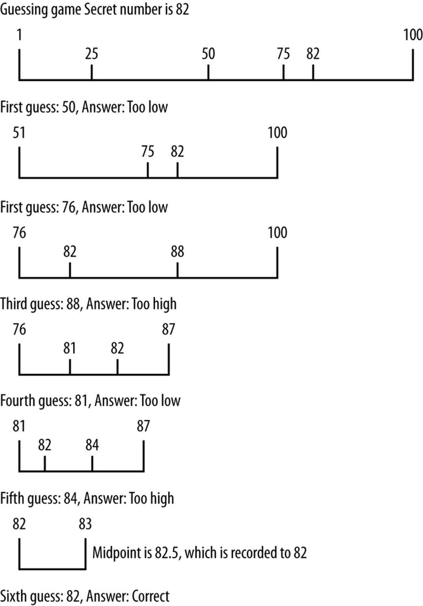
Figure 13-2. Binary search algorithm applied to guessing a number
We can implement this strategy as the binary search algorithm. This algorithm only works on a sorted data set. Here is the algorithm:
1. Set a lower bound to the first position of the array (0).
2. Set an upper bound to the last element of the array (length of array minus 1).
3. While the lower bound is less than or equal to the upper bound, do the following steps:
a. Set the midpoint as (upper bound minus lower bound) divided by 2.
b. If the midpoint element is less than the data being searched for, set a new lower bound to the midpoint plus 1.
c. If the midpoint element is greater than the data being searched for, set a new upper bound to the midpoint minus 1.
d. Otherwise, return the midpoint as the found element.
Example 13-12 shows the JavaScript definition for the binary search algorithm, along with a program to test the definition.
Example 13-12. Using the binary search algorithm
function binSearch(arr, data) {
var upperBound = arr.length-1;
var lowerBound = 0;
while (lowerBound <= upperBound) {
var mid = Math.floor((upperBound + lowerBound) / 2);
if (arr[mid] < data) {
lowerBound = mid + 1;
}
else if (arr[mid] > data) {
upperBound = mid - 1;
}
else {
return mid;
}
}
return -1;
}
var nums = [];
for (var i = 0; i < 100; ++i) {
nums[i] = Math.floor(Math.random() * 101);
}
insertionsort(nums);
dispArr(nums);
print();
putstr("Enter a value to search for: ");
var val = parseInt(readline());
var retVal = binSearch(nums, val);
if (retVal >= 0) {
print("Found " + val + " at position " + retVal);
}
else {
print(val + " is not in array.");
}
Here is the output from one run of the program:
0 1 2 3 5 7 7 8 8 9 10
11 11 13 13 13 14 14 14 15 15
18 18 19 19 19 19 20 20 20 21
22 22 22 23 23 24 25 26 26 29
31 31 33 37 37 37 38 38 43 44
44 45 48 48 49 51 52 53 53 58
59 60 61 61 62 63 64 65 68 69
70 72 72 74 75 77 77 79 79 79
83 83 84 84 86 86 86 91 92 93
93 93 94 95 96 96 97 98 100
Enter a value to search for: 37
Found 37 at position 45
It will be interesting to watch the function as it works its way through the search space looking for the value specified, so in Example 13-13, let’s add a statement to the binSearch() function that displays the midpoint each time it is recalculated:
Example 13-13. binSearch() displaying the midpoint value
function binSearch(arr, data) {
var upperBound = arr.length-1;
var lowerBound = 0;
while (lowerBound <= upperBound) {
var mid = Math.floor((upperBound + lowerBound) / 2);
print("Current midpoint: " + mid);
if (arr[mid] < data) {
lowerBound = mid + 1;
}
else if (arr[mid] > data) {
upperBound = mid - 1;
}
else {
return mid;
}
}
return -1;
}
Now let’s run the program again:
0 0 2 3 5 6 7 7 7 10 11
14 14 15 16 18 18 19 20 20 21
21 21 22 23 24 26 26 27 28 28
30 31 32 32 32 32 33 34 35 36
36 37 37 38 38 39 41 41 41 42
43 44 47 47 50 51 52 53 56 58
59 59 60 62 65 66 66 67 67 67
68 68 68 69 70 74 74 76 76 77
78 79 79 81 81 81 82 82 87 87
87 87 92 93 95 97 98 99 100
Enter a value to search for: 82
Current midpoint: 49
Current midpoint: 74
Current midpoint: 87
Found 82 at position 87
From this output, we see that the original midpoint value was 49. That’s too low since we are searching for 82, so the next midpoint is calculated to be 74. That’s still too low, so a new midpoint is calculated, 87, and that value holds the element we are searching for, so the search is over.
Counting Occurrences
When the binSearch() function finds a value, if there are other occurrences of the same value in the data set, the function will be positioned in the immediate vicinity of other like values. In other words, other occurrences of the same value will either be to the immediate left of the found value’s position or to the immediate right of the found value’s position.
If this fact isn’t readily apparent to you, run the binSearch() function several times and take note of the position of the found value returned by the function. Here’s an example of a sample run from earlier in this chapter:
0 1 2 3 5 7 7 8 8 9 10
11 11 13 13 13 14 14 14 15 15
18 18 19 19 19 19 20 20 20 21
22 22 22 23 23 24 25 26 26 29
31 31 33 37 37 37 38 38 43 44
44 45 48 48 49 51 52 53 53 58
59 60 61 61 62 63 64 65 68 69
70 72 72 74 75 77 77 79 79 79
83 83 84 84 86 86 86 91 92 93
93 93 94 95 96 96 97 98 100
Enter a value to search for: 37
Found 37 at position 45
If you count the position of each element, the number 37 found by the function is the one that is in the middle of the three occurrences of 37. This is just the nature of how the binSearch() function works.
So what does a function that counts the occurrences of values in a data set need to do to make sure that it counts all the occurrences? The easiest solution is to write two loops that move both down, or to the left of, the data set, counting occurrences, and up, or the right of, the data set, counting occurrences. Example 13-14 shows a definition of the count() function.
Example 13-14. The count() function
function count(arr, data) {
var count = 0;
var position = binSearch(arr, data);
if (position > -1) {
++count;
for (var i = position-1; i > 0; --i) {
if (arr[i] == data) {
++count;
}
else {
break;
}
}
for (var i = position+1; i < arr.length; ++i) {
if (arr[i] == data) {
++count;
}
else {
break;
}
}
}
return count;
}
The function starts by calling the binSearch() function to search for the specified value. If the value is found in the data set, the the function begins counting occurrences by calling two for loops. The first loop works its way down the array, counting occurrences of the found value, stopping when the next value in the array doesn’t match the found value. The second for loop works its way up the array, counting occurrences and stopping when the next value in the array doesn’t match the found value.
Example 13-15 shows how we can use count() in a program.
Example 13-15. Using the count() function
var nums = [];
for (var i = 0; i < 100; ++i) {
nums[i] = Math.floor(Math.random() * 101);
}
insertionsort(nums);
dispArr(nums);
print();
putstr("Enter a value to count: ");
var val = parseInt(readline());
var retVal = count(nums, val);
print("Found " + retVal + " occurrences of " + val + ".");
Here is a sample run of the program:
0 1 3 5 6 8 8 9 10 10 10
12 12 13 15 18 18 18 20 21 21
22 23 24 24 24 25 27 27 30 30
30 31 32 35 35 35 36 37 40 40
41 42 42 44 44 45 45 46 47 48
51 52 55 56 56 56 57 58 59 60
61 61 61 63 64 66 67 69 69 70
70 72 72 73 74 74 75 77 78 78
78 78 82 82 83 84 87 88 92 92
93 94 94 96 97 99 99 99 100
Enter a value to count: 45
Found 2 occurrences of 45.
Here is another sample run:
0 1 1 2 2 3 6 7 7 7 7
8 8 8 11 11 11 11 11 12 14
15 17 18 18 18 19 19 23 25 27
28 29 30 30 31 32 32 32 33 36
36 37 37 38 38 39 43 43 43 45
47 48 48 48 49 50 53 55 55 55
59 59 60 62 65 66 67 67 71 72
73 73 75 76 77 79 79 79 79 83
85 85 87 88 89 92 92 93 93 93
94 94 94 95 96 97 98 98 99
Enter a value to count: 56
Found 0 occurrences of 56.
Searching Textual Data
Up to this point, all of our searches have been conducted on numeric data. We can also use the algorithms discussed in this chapter with textual data. First, let’s define the data set we are using:
The nationalism of Hamilton was undemocratic. The democracy of Jefferson was,
in the beginning, provincial. The historic mission of uniting nationalism and
democracy was in the course of time given to new leaders from a region beyond
the mountains, peopled by men and women from all sections and free from those
state traditions which ran back to the early days of colonization. The voice
of the democratic nationalism nourished in the West was heard when Clay of
Kentucky advocated his American system of protection for industries; when
Jackson of Tennessee condemned nullification in a ringing proclamation that
has taken its place among the great American state papers; and when Lincoln
of Illinois, in a fateful hour, called upon a bewildered people to meet the
supreme test whether this was a nation destined to survive or to perish. And
it will be remembered that Lincoln's party chose for its banner that earlier
device--Republican--which Jefferson had made a sign of power. The "rail splitter"
from Illinois united the nationalism of Hamilton with the democracy of Jefferson,
and his appeal was clothed in the simple language of the people, not in the
sonorous rhetoric which Webster learned in the schools.
This paragraph of text was taken from the big.txt file found on Peter Norvig’s website. This file is stored as a text file (.txt) that is located in the same directory as the JavaScript interpreter (js.exe).
To read the file into a program, we need just one line of code:
var words = read("words.txt").split(" ");
This line stores the text in an array by reading in the text from the file—read("words.txt")—and then breaking up the file into words using the split() function, which uses the space between each word as the delimiter. This code is not perfect because puncuation is left in the file and is stored with the nearest word, but it will suffice for our purposes.
Once the file is stored in an array, we can begin searching through the array to find words. Let’s begin with a sequential search and search for the word “rhetoric,” which is in the paragraph close to the end of the file. Let’s also time the search so we can compare it with a binary search. We covered timing code in Chapter 12 if you want to go back and review that material. Example 13-16 shows the code.
Example 13-16. Searching a text file using seqSearch()
function seqSearch(arr, data) {
for (var i = 0; i < arr.length; ++i) {
if (arr[i] == data) {
return i;
}
}
return -1;
}
var words = read("words.txt").split(" ");
var word = "rhetoric";
var start = new Date().getTime();
var position = seqSearch(words, word);
var stop = new Date().getTime();
var elapsed = stop - start;
if (position >= 0) {
print("Found " + word + " at position " + position + ".");
print("Sequential search took " + elapsed + " milliseconds.");
}
else {
print(word + " is not in the file.");
}
The output from this program is:
Found rhetoric at position 174.
Sequential search took 0 milliseconds.
Even though binary search is faster, we won’t be able to measure any difference between seqSearch() and binSearch(), but we will run the program using binary search anyway to ensure that the binSearch() function works correctly with text. Example 13-17 shows the code and the output.
Example 13-17. Searching textual data with binSearch()
function binSearch(arr, data) {
var upperBound = arr.length-1;
var lowerBound = 0;
while (lowerBound <= upperBound) {
var mid = Math.floor((upperBound + lowerBound) / 2);
if (arr[mid] < data) {
lowerBound = mid + 1;
}
else if (arr[mid] > data) {
upperBound = mid - 1;
}
else {
return mid;
}
}
return -1;
}
function insertionsort(arr) {
var temp, inner;
for (var outer = 1; outer <= arr.length-1; ++outer) {
temp = arr[outer];
inner = outer;
while (inner > 0 && (arr[inner-1] >= temp)) {
arr[inner] = arr[inner-1];
--inner;
}
arr[inner] = temp;
}
}
var words = read("words.txt").split(" ");
insertionsort(words);
var word = "rhetoric";
var start = new Date().getTime();
var position = binSearch(words, word);
var stop = new Date().getTime();
var elapsed = stop - start;
if (position >= 0) {
print("Found " + word + " at position " + position + ".");
print("Binary search took " + elapsed + " milliseconds.");
}
else {
print(word + " is not in the file.");
}
Found rhetoric at position 124.
Binary search took 0 milliseconds.
In this age of superfast processors, it is harder and harder to measure the difference between sequential search and binary search on anything but the largest data sets. However, it has been proven mathematically that binary search is faster than sequential search on large data sets just due to the fact that the binary search algorithm eliminates half the search space (the elements of the array) with each iteration of the loop that controls the algorithm.
Exercises
1. The sequential search algorithm always finds the first occurrence of an element in a data set. Rewrite the algorithm so that the last occurrence of an element is returned.
2. Compare the time it takes to perform a sequential search with the total time it takes to both sort a data set using insertion sort and perform a binary search on the data set. What are your results?
3. Create a function that finds the second-smallest element in a data set. Can you generalize the function definition for the third-smallest, fourth-smallest, and so on? Test your functions with a data set of at least 1,000 elements. Test on both numbers and text.
All materials on the site are licensed Creative Commons Attribution-Sharealike 3.0 Unported CC BY-SA 3.0 & GNU Free Documentation License (GFDL)
If you are the copyright holder of any material contained on our site and intend to remove it, please contact our site administrator for approval.
© 2016-2026 All site design rights belong to S.Y.A.