Data Structures and Algorithms with JavaScript (2014)

Chapter 14. Advanced Algorithms

In this chapter we’ll look at two advanced topics: dynamic programming and greedy algorithms. Dynamic programming is a technique that is sometimes considered the opposite of recursion. Where a recursive solution starts at the top and breaks the problem down, solving all small problems until the complete problem is solved, a dynamic programming solution starts at the bottom, solving small problems and combining them to form an overall solution to the big problem. This chapter departs from most of the other chapters in this book in that we don’t really discuss an organizing data structure for working with these algorithms other than the array. Sometimes, a simple data structure is enough to solve a problem if the algorithm you are using is powerful enough.

A greedy algorithm is an algorithm that looks for “good solutions” as it works toward the complete solution. These good solutions, called local optima, will hopefully lead to the correct final solution, called the global optimum. The term “greedy” comes from the fact that these algorithms take whatever solution looks best at the time. Often, greedy algorithms are used when it is almost impossible to find a complete solution, owing to time and/or space considerations, and yet a suboptimal solution is acceptable.

A good source for more information on advanced algorithms and data structures is Introduction to Algorithms (MIT Press).

Dynamic Programming

Recursive solutions to problems are often elegant but inefficient. Many languages, including JavaScript, cannot efficiently translate recursive code to machine code, resulting in an inefficient though elegant computer program. This is not to say that using recursion is bad, per se, just that some imperative and object-oriented programming languages do not do a good job implementing recursion, since they do not feature recursion as a high-priority programming technique.

Many programming problems that have recursive solutions can be rewritten using the techniques of dynamic programming. A dynamic programming solution builds a table, usually using an array, that holds the results of the many subsolutions as the problem is broken down. When the algorithm is complete, the solution is found in a distinct spot in the table, as we’ll see in the Fibonacci example next.

A Dynamic Programming Example: Computing Fibonacci Numbers

The Fibonacci numbers can be defined by the following sequence:

0, 1, 1, 2, 3, 5, 8, 13, 21, 34, 55, …

As you can tell, the sequence is generated by adding the previous two numbers in the sequence together. This sequence has a long history dating back to at least 700 AD and is named after the Italian mathematician Leornardo Fibonacci, who in 1202 used the sequence to describe the idealized growth of a rabbit population.

There is a simple recursive solution you can use to generate any specific number in the sequence. Here is the JavaScript code for a Fibonacci function:

function recurFib(n) {

if (n < 2) {

return n;

}

else {

return recurFib(n-1) + recurFib(n-2);

}

}

print(recurFib(10)); // displays 55

The problem with this function is that it is extremely inefficient. We can see exactly how inefficient it is by examining the recursion tree shown in Figure 14-1 for fib(5).

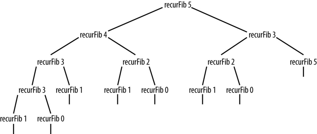
Figure 14-1. Recursion tree generated by recursive Fibonacci function

It is clear that too many values are recomputed during the recursive calls. If the compiler could keep track of the values that are already computed, the function would not be nearly so inefficient. We can design a much more efficient algorithm using dynamic programming techniques.

An algorithm designed using dynamic programming starts by solving the simplest subproblem it can solve, then using that solution to solve more complex subproblems until the entire problem is solved. The solutions to each subproblem are typically stored in an array for easy access.

We can demonstrate the essence of dynamic programming by examing the dynamic programming solution to computing Fibonacci numbers, as shown in the function definition in the following section:

function dynFib(n) {

var val = [];

for (var i = 0; i <= n; ++i) {

val[i] = 0;

}

if (n == 1 || n == 2) {

return 1;

}

else {

val[1] = 1;

val[2] = 2;

for (var i = 3; i <= n; ++i) {

val[i] = val[i-1] + val[i-2];

}

return val[n-1];

}

}

The val array is where we store intermediate results. The first part of the if statement returns the value 1 if the Fibonacci number to be computed is 1 or 2. Otherwise, the values 1 and 2 are stored in positions 1 and 2 of val. The for loop runs from 3 to the input argument, assigning each array element the sum of the previous two array elements, and when the loop is complete, the last value in the array will be the last computed Fibonacci number, which is the number asked for and is the value returned by the function.

The arrangement of the Fibonacci sequence in the val array is shown here:

val[0] = 0 val[1] = 1 val[2] = 2 val[3] = 3 val[4] = 5 val[5] = 8 val[6] = 13

Let’s compare the time it takes to compute a Fibonacci number using both the recursive function and the dynamic programming function. Example 14-1 lists the code for the timing test.

Example 14-1. Timing test for recursive and dynamic programming versions of Fibonacci function

function recurFib(n) {

if (n < 2) {

return n;

}

else {

return recurFib(n-1) + recurFib(n-2);

}

}

function dynFib(n) {

var val = [];

for (var i = 0; i <= n; ++i) {

val[i] = 0;

}

if (n == 1 || n == 2) {

return 1;

}

else {

val[1] = 1;

val[2] = 2;

for (var i = 3; i <= n; ++i) {

val[i] = val[i-1] + val[i-2];

}

return val[n-1];

}

}

var start = new Date().getTime();

print(recurFib(10));

var stop = new Date().getTime();

print("recursive time - " + (stop-start) + "milliseconds");

print();

start = new Date().getTime();

print(dynFib(10));

stop = new Date().getTime();

print("dynamic programming time - " + (stop-start) + " milliseconds");

The output from this program is:

832040

recursive time - 0 milliseconds

832040

dynamic programming time - 0 milliseconds

If we run the program again, this time computing fib(20), we get:

6765

recursive time - 1 milliseconds

6765

dynamic programming time - 0 milliseconds

Finally, we compute fib(30) and we get:

832040

recursive time - 17 milliseconds

832040

dynamic programming time - 0 milliseconds

Clearly, the dynamic programming solution is much more efficient than the recursive solution when we compute anything over fib(20).

Finally, you may have already figured out that it’s not necessary to use an array when computing a Fibonacci number using the iterative solution. The array was used because dynamic programming algorithms usually store intermediate results in an array. Here is the definition of an iterative Fibonacci function that doesn’t use an array:

function iterFib(n) {

var last = 1;

var nextLast = 1;

var result = 1;

for (var i = 2; i < n; ++i) {

result = last + nextLast;

nextLast = last;

last = result;

}

return result;

}

This version of the function will compute Fibonacci numbers as efficiently as the dynamic programming version.

Finding the Longest Common Substring

Another problem that lends itself to a dynamic programming solution is finding the longest common substring in two strings. For example, in the words “raven” and “havoc,” the longest common substring is “av.” A common use of finding the longest common substring is in genetics, where DNA molecules are described using the first letter of the nucleobase of a nucleotide.

We’ll start with the brute-force solution to this problem. Given two strings, A and B, we can find the longest common substring by starting at the first character of A and comparing each character to the corresponding character of B. When a nonmatch is found, move to the second character of A and start over with the first character of B, and so on.

There is a better solution using dynamic programming. The algorithm uses a two-dimensional array to store the results of comparisons of the characters in the same position in the two strings. Initially, each element of the array is set to 0. Each time a match is found in the same position of the two arrays, the element at the corresponding row and column of the array is incremented by 1; otherwise the element stays set to 0. Along the way, a variable is keeping track of how many matches are found. This variable, along with an indexing variable, are used to retrieve the longest common substring once the algorithm is finished.

Example 14-2 presents the complete definition of the algorithm. After the code, we’ll explain how it works.

Example 14-2. A function for determining the longest common substring of two strings

function lcs(word1, word2) {

var max = 0;

var index = 0;

var lcsarr = new Array(word1.length+1);

for (var i = 0; i <= word1.length+1; ++i) {

lcsarr[i] = new Array(word2.length+1);

for (var j = 0; j <= word2.length+1; ++j) {

lcsarr[i][j] = 0;

}

}

for (var i = 0; i <= word1.length; ++i) {

for (var j = 0; j <= word2.length; ++j) {

if (i == 0 || j == 0) {

lcsarr[i][j] = 0;

}

else {

if (word1[i-1] == word2[j-1]) {

lcsarr[i][j] = lcsarr[i-1][j-1] + 1;

}

else {

lcsarr[i][j] = 0;

}

}

if (max < lcsarr[i][j]) {

max = lcsarr[i][j];

index = i;

}

}

}

var str = "";

if (max == 0) {

return "";

}

else {

for (var i = index-max; i <= max; ++i) {

str += word2[i];

}

return str;

}

}

The first section of the function sets up a couple of variables and the two-dimensional array. Most languages have a simple declaration for two-dimensional arrays, but JavaScript makes you jump through a few hoops by declaring an array inside an array. The last for loop in the code fragment initializes the array. Here’s the first section:

function lcs(word1, word2) {

var max = 0;

var index = 0;

var lcsarr = new Array(word1.length+1);

for (var i = 0; i <= word1.length+1; ++i) {

lcsarr[i] = new Array(word2.length+1);

for (var j = 0; j <= word2.length+1; ++j) {

lcsarr[i][j] = 0;

}

}

Now here is the code for the second section of the function:

for (var i = 0; i <= word1.length; ++i) {

for (var j = 0; j <= word2.length; ++j) {

if (i == 0 || j == 0) {

lcsarr[i][j] = 0;

}

else {

if (word1[i-1] == word2[j-1]) {

lcsarr[i][j] = lcsarr[i-1][j-1] + 1;

}

else {

lcsarr[i][j] = 0;

}

}

if (max < lcsarr[i][j]) {

max = lcsarr[i][j];

index = i;

}

}

}

The second section builds the table that keeps track of character matches. The first elements of the array are always set to 0. Then if the corresponding characters of the two strings match, the current array element is set to 1 plus the value stored in the previous array element. For example, if the two strings are “back” and “cace,” and the algorithm is on the second character, then a 1 is placed in the current element, since the previous element wasn’t a match and a 0 is stored in that element (0 + 1). The algorithm then moves to the next position, and since it also matches for both strings, a 2 is placed in the current array element (1 + 1). The last characters of the two strings don’t match, so the longest common substring is 2. Finally, if max is less than the value now stored in the current array element, it is assigned the value of the current array element, and index is set to the current value of i. These two variables will be used in the last section to determine where to start retrieving the longest common substring.

For example, given the two strings “abbcc” and “dbbcc,” here is the state of the lcsarr array as the algorithm progresses:

0 0 0 0 0

0 0 0 0 0

0 1 1 0 0

0 1 2 0 0

0 0 0 3 1

0 0 0 1 4

The last section builds the longest common substring by determining where to start. The value of index minus max is the starting point, and the value of max is the stopping point:

var str = "";

if (max == 0) {

return "";

}

else {

for (var i = index-max; i <= max; ++i) {

str += word2[i];

}

return str;

}

Given again the two strings “abbcc” and “dbbcc,” the program returns “bbcc.”

The Knapsack Problem: A Recursive Solution

A classic problem in the study of algorithms is the knapsack problem. Imagine you are a safecracker and you break open a safe filled with all sorts of treasure, but all you have to carry the loot is a small backpack. The items in the safe differ in both size and value. You want to maximize your take by filling the backpack with those items that are worth the most.

There is, of course, a brute-force solution to this problem, but the dynamic programming solution is more efficient. The key idea to solving the knapsack problem with a dynamic programming solution is to calculate the maximum value for every item up to the total capacity of the knapsack.

If the safe in our example has five items, the items have a size of 3, 4, 7, 8, and 9, respectively, and values of 4, 5, 10, 11, and 13, respectively, and the knapsack has a capacity of 16, then the proper solution is to pick items 3 and 5 with a total size of 16 and a total value of 23.

The code for solving this problem is quite short, but it won’t make much sense without the context of the whole program, so let’s take a look at the program to solve the knapsack problem. Our solution uses a recursive function:

function max(a, b) {

return (a > b) ? a : b;

}

function knapsack(capacity, size, value, n) {

if (n == 0 || capacity == 0) {

return 0;

}

if (size[n-1] > capacity) {

return knapsack(capacity, size, value, n-1);

}

else {

return max(value[n-1] +

knapsack(capacity-size[n-1], size, value, n-1),

knapsack(capacity, size, value, n-1));

}

}

var value = [4,5,10,11,13];

var size = [3,4,7,8,9];

var capacity = 16;

var n = 5;

print(knapsack(capacity, size, value, n));

The output from this program is:

23

The problem with this recursive solution to the knapsack problem is that, because it is recursive, many subproblems are revisited during the course of the recursion. A better solution to the knapsack problem is to use a dynamic programming technique to solve the problem, as shown below.

The Knapsack Problem: A Dynamic Programming Solution

Whenever we find a recursive solution to a problem, we can usually rewrite the solution using a dynamic programming technique and end up with a more efficient program. The knapsack problem can definitely be rewritten in a dynamic programming manner. All we have to do is use an array to store temporary solutions until we get to the final solution.

The following program demonstrates how the knapsack problem we encountered earlier can be solved using dynamic programming. The optimum value for the given constraints is, again, 23. Example 14-3 shows the code.

Example 14-3. A dynamic programming solution to the knapsack problem

function max(a, b) {

return (a > b) ? a : b;

}

function dKnapsack(capacity, size, value, n) {

var K = [];

for (var i = 0; i <= capacity+1; i++) {

K[i] = [];

}

for (var i = 0; i <= n; i++) {

for (var w = 0; w <= capacity; w++) {

if (i == 0 || w == 0) {

K[i][w] = 0;

}

else if (size[i-1] <= w) {

K[i][w] = max(value[i-1] + K[i-1][w-size[i-1]],

K[i-1][w]);

}

else {

K[i][w] = K[i-1][w];

}

putstr(K[i][w] + " ");

}

print();

}

return K[n][capacity];

}

var value = [4,5,10,11,13];

var size = [3,4,7,8,9];

var capacity = 16;

var n = 5;

print(dKnapsack(capacity, size, value, n));

As the program runs, it displays the values being stored in the table as the algorithm works toward a solution. Here is the output:

0 0 0 0 0 0 0 0 0 0 0 0 0 0 0 0 0

0 0 0 4 4 4 4 4 4 4 4 4 4 4 4 4 4

0 0 0 4 5 5 5 9 9 9 9 9 9 9 9 9 9

0 0 0 4 5 5 5 10 10 10 14 15 15 15 19 19 19

0 0 0 4 5 5 5 10 11 11 14 15 16 16 19 21 21

0 0 0 4 5 5 5 10 11 13 14 15 17 18 19 21 23

23

The optimal solution to the problem is found in the last cell of the two-dimensional table, which is found in the bottom-right corner of the table. You will also notice that using this technique does not tell you which items to pick to maximize output, but from inspection, the solution is to pick items 3 and 5, since the capacity is 16, item 3 has a size 7 (value 10), and item 5 has a size 9 (value 13).

Greedy Algorithms

In the previous sections, we examined dynamic programming algorithms that can be used to optimize solutions that are found using a suboptimal algorithm—solutions that are often based on recursion. For many problems, resorting to dynamic programming is overkill and a simpler algorithm will suffice.

One example of a simpler algorithm is the greedy algorithm. A greedy algorithm is one that always chooses the best solution at the time, with no regard to how that choice will affect future choices. Using a greedy algorithm generally indicates that the implementer hopes that the series of “best” local choices made will lead to a final “best” choice. If so, then the algorithm has produced an optimal solution; if not, a suboptimal solution has been found. However, for many problems, it is just not worth the trouble to find an optimal solution, so using a greedy algorithm works just fine.

A First Greedy Algorithm Example: The Coin-Changing Problem

A classic example of following a greedy algorithm is making change. Let’s say you buy some items at the store and the change from your purchase is 63 cents. How does the clerk determine the change to give you? If the clerk follows a greedy algorithm, he or she gives you two quarters, a dime, and three pennies. That is the smallest number of coins that will equal 63 cents without using half-dollars.

Example 14-4 demonstrates a program that uses a greedy algorithm to make change (under the assumption that the amount of change is less than one dollar).

Example 14-4. A greedy algorithm for solving the coin-changing problem

function makeChange(origAmt, coins) {

var remainAmt = 0;

if (origAmt % .25 < origAmt) {

coins[3] = parseInt(origAmt / .25);

remainAmt = origAmt % .25;

origAmt = remainAmt;

}

if (origAmt % .1 < origAmt) {

coins[2] = parseInt(origAmt / .1);

remainAmt = origAmt % .1;

origAmt = remainAmt;

}

if (origAmt % .05 < origAmt) {

coins[1] = parseInt(origAmt / .05);

remainAmt = origAmt % .05;

origAmt = remainAmt;

}

coins[0] = parseInt(origAmt / .01);

}

function showChange(coins) {

if (coins[3] > 0) {

print("Number of quarters - " + coins[3] + " - " + coins[3] * .25);

}

if (coins[2] > 0) {

print("Number of dimes - " + coins[2] + " - " + coins[2] * .10);

}

if (coins[1] > 0) {

print("Number of nickels - " + coins[1] + " - " + coins[1] * .05);

}

if (coins[0] > 0) {

print("Number of pennies - " + coins[0] + " - " + coins[0] * .01);

}

}

var origAmt = .63;

var coins = [];

makeChange(origAmt, coins);

showChange(coins);

The output from this program is:

Number of quarters - 2 - 0.5

Number of dimes - 1 - 0.1

Number of pennies - 3 - 0.03

The makeChange() function starts with the highest denomination, quarters, and tries to make as much change with them as possible. The total number of quarters is stored in the coins array. Once the amount left becomes less than a quarter, the algorithm moves to dimes, making as much change with dimes as possible. The total number of dimes is then stored in the coins array. The algorithm then moves to nickels and pennies in the same manner.

This solution always finds the optimal solution as long as the normal coin denominations are used and all the possible denominations are available. Not being able to use one particular denomination, such as nickels, can lead to a suboptimal solution.

A Greedy Algorithm Solution to the Knapsack Problem

Earlier in this chapter we examined the knapsack problem and provided both recursive and dynamic programming solutions for it. In this section, we’ll examine how we can implement a greedy algorithm to solve this problem.

A greedy algorithm can be used to solve the knapsack problem if the items we are placing in the knapsack are continuous in nature. In other words, the items must be things that cannot be counted discretely, such as cloth or gold dust. If we are using continous items, we can simply divide the unit price by the unit volume to determine the value of the item. An optimal solution in this case is to place as much of the item with the highest value into the knapsack as possible until the item is depleted or the knapsack is full, followed by as much of the second-highest-value item as possible, and so on. The reason we can’t find an optimal greedy solution using discrete items is because we can’t put “half a television” into a knapsack. Discrete knapsack problems are known as 0-1 problems because you must take either all or none of an item.

This type of knapsack problem is called a fractional knapsack problem. Here is the algorithm for solving fractional knapsack problems:

1. Knapsack has a capacity W and items have values V and weights w.

2. Rank items by v/w ratio.

3. Consider items in terms of decreasing ratio.

4. Take as much of each item as possible.

Table 14-1 gives the weights, values, and ratios for four items.

Table 14-1. Fractional knapsack items

Given the table above, and assuming that the knapsack being used has a capacity of 30, the optimal solution for the knapsack problem is to take all of item A, all of item B, and half of item C. This combination of items will result in a value of 220.

The code for finding the optimal solution to this knapsack problem is shown below:

function ksack(values, weights, capacity) {

var load = 0;

var i = 0;

var w = 0;

while (load < capacity && i < 4) {

if (weights[i] <= (capacity-load)) {

w += values[i];

load += weights[i];

}

else {

var r = (capacity-load)/weights[i];

w += r * values[i];

load += weights[i];

}

++i;

}

return w;

}

var items = ["A", "B", "C", "D"];

var values = [50, 140, 60, 60];

var weights = [5, 20, 10, 12];

var capacity = 30;

print(ksack(values, weights, capacity)); // displays 220

Exercises

1. Write a program that uses a brute-force technique to find the longest common substring.

2. Write a program that allows the user to change the constraints of a knapsack problem in order to explore how changing the constraints will change the results of the solution. For example, you can change the capacity of the knapsack, the values of the items, or the weights of the items. It is probably a good idea to change only one of these constraints at a time.

3. Using the greedy algorithm technique for coin changing, but not allowing the algorithm to use dimes, find the solution for 30 cents. Is this solution optimal?