Running Linux, 5th Edition (2009)
Part III. Programming
The tools and practices in this part of the book are not needed by all users, but anyone willing to master them can add a great deal of power to their system. If you've done programming before, this part of the book gets you to a productive state on Linux quickly; if you haven't, it can show you some of the benefits of programming and serve as an introduction to its joys. Chapter 20 shows you two great tools for text editing--vi and Emacs—that you should master even if you don't plan to be a programmer. The material in this part of the book can also be a valuable reference as you read other parts.
Chapter 21: Programming Tools
Chapter 22: Running a Web Server
Chapter 23: Transporting and Handling Email Messages
Chapter 24: SRunning an FTP Server
Chapter 21. Programming Tools
There's much more to Linux than simply using the system. One of the benefits of free software is that you can modify it to suit your needs. This applies equally to the many free applications available for Linux and to the Linux kernel itself.
Linux supports an advanced programming interface, using GNU compilers and tools, such as the gcc compiler, the gdb debugger, and so on. An enormous number of other programming languages—ranging from such classics as FORTRAN and LISP to modern scripting languages such as Perl, Python, and Ruby—are also supported. Whatever your programming needs, Linux is a great choice for developing Unix applications. Because the complete source code for the libraries and Linux kernel is provided, programmers who need to delve into the system internals are able to do so.[*]
Many judge a computer system by the tools it offers its programmers. Unix systems have won the contest by many people's standards, having developed a very rich set over the years. Leading the parade is the GNU debugger, gdb. In this chapter, we take a close look at this invaluable utility, and at a number of other auxiliary tools C programmers will find useful.
Even if you are not a programmer, you should consider using the Revision Control System (RCS ). It provides one of the most reassuring protections a computer user could ask for—backups for everything you do to a file. If you delete a file by accident, or decide that everything you did for the past week was a mistake and should be ripped out, RCS can recover any version you want. If you are working on a larger project that involves either a large number of developers or a large number of directories (or both), Concurrent Versioning System (CVS) might be more suitable for you. It was originally based on RCS, but was rewritten from the ground up and provides many additional features. Currently, another tool, called Subversion, is taking over from CVS and filling in some of the gaps that CVS left in the handling of large projects.[*] The goal of Subversion is to be "like CVS; just better." Newer installations typically use Subversion these days, but the vast majority still uses CVS. Finally, the Linux kernel itself uses yet another versioning system. It used to use a software called BitKeeper, but when licensing problems arose, Linus Torvalds wrote his own version control system, called git, that has been introduced recently.
Linux is an ideal platform for developing software to run under the X Window System. The Linux X distribution, as described in Chapter 16, is a complete implementation with everything you need to develop and support X applications. Programming for X is portable across applications, so the X-specific portions of your application should compile cleanly on other Unix systems.
In this chapter, we explore the Linux programming environment and give you a five-cent tour of the many facilities it provides. Half of the trick to Unix programming is knowing what tools are available and how to use them effectively. Often the most useful features of these tools are not obvious to new users.
Since C programming has been the basis of most large projects (even though it is nowadays being replaced more and more by C++ and Java ) and is the language common to most modern programmers—not only on Unix, but on many other systems as well—we start by telling you what tools are available for that. The first few sections of the chapter assume you are already a C programmer.
But several other tools are emerging as important resources, especially for system administration. We examine one in this chapter: Perl. Perl is a scripting language like the Unix shells, taking care of grunt work such as memory allocation so you can concentrate on your task. But Perl offers a degree of sophistication that makes it more powerful than shell scripts and therefore appropriate for many programming tasks.
Several open source projects make it relatively easy to program in Java, and some of the tools and frameworks in the open source community are even more popular than those distributed by Sun Microsystems, the company that invented and licenses Java. Java is a general-purpose language with many potential Internet uses. In a later section, we explore what Java offers and how to get started.
Programming with gcc
The C programming language is by far the most often used in Unix software development. Perhaps this is because the Unix system was originally developed in C; it is the native tongue of Unix. Unix C compilers have traditionally defined the interface standards for other languages and tools, such as linkers, debuggers, and so on. Conventions set forth by the original C compilers have remained fairly consistent across the Unix programming board.
gcc is one of the most versatile and advanced compilers around. Unlike other C compilers (such as those shipped with the original AT&T or BSD distributions, or those available from various third-party vendors), gcc supports all the modern C standards currently in use—such as the ANSI C standard—as well as many extensions specific to gcc. Happily, however, gcc provides features to make it compatible with older C compilers and older styles of C programming. There is even a tool called protoize that can help you write function prototypes for old-style C programs.
gcc is also a C++ compiler. For those who prefer the more modern object-oriented environment, C++ is supported with all the bells and whistles—including most of the C++ introduced when the C++ standard was released, such as method templates. Complete C++ class libraries are provided as well, such as the Standard Template Library (STL).
For those with a taste for the particularly esoteric, gcc also supports Objective-C, an object-oriented C spinoff that never gained much popularity but may see a second spring due to its usage in Mac OS X. And there is gcj, which compiles Java code to machine code. But the fun doesn't stop there, as we'll see.
In this section, we cover the use of gcc to compile and link programs under Linux. We assume you are familiar with programming in C/C++, but we don't assume you're accustomed to the Unix programming environment. That's what we introduce here.
Warning
The latest gcc version at the time of this writing is Version 4.0. However, this is still quite new, sometimes a bit unstable, and, since it is a lot stricter about syntax than previous versions, will not compile some older code. Many developers therefore use either a version of the 3.3 series (with 3.3.5 being the current one at the time of this writing) or Version 3.4. We suggest sticking with either of those unless you know exactly what you are doing.
A word about terminology ahead: Because gcc can these days compile so much more than C (for example, C++, Java, and some other programming languages), it is considered to be the abbreviation for GNU Compiler Collection. But if you speak about just the C compiler, gcc is taken to mean GNU C Compiler.
Quick Overview
Before imparting all the gritty details of gcc, we present a simple example and walk through the steps of compiling a C program on a Unix system.
Let's say you have the following bit of code, an encore of the much overused "Hello, World!" program (not that it bears repeating):
#include <stdio.h>
int main() {
(void)printf("Hello, World!\n");
return 0; /* Just to be nice */
}
Several steps are required to compile this program into a living, breathing executable. You can accomplish most of these steps through a single gcc command, but we've left the specifics for later in the chapter.
First, the gcc compiler must generate an object file from this source code . The object file is essentially the machine-code equivalent of the C source. It contains code to set up the main() calling stack, a call to the printf() function, and code to return the value of 0.
The next step is to link the object file to produce an executable. As you might guess, this is done by the linker. The job of the linker is to take object files , merge them with code from libraries , and spit out an executable. The object code from the previous source does not make a complete executable. First and foremost, the code for printf() must be linked in. Also, various initialization routines, invisible to the mortal programmer, must be appended to the executable.
Where does the code for printf() come from? Answer: the libraries. It is impossible to talk for long about gcc without mentioning them. A library is essentially a collection of many object files, including an index. When searching for the code for printf(), the linker looks at the index for each library it's been told to link against. It finds the object file containing the printf() function and extracts that object file (the entire object file, which may contain much more than just the printf() function) and links it to the executable.
In reality, things are more complicated than this. Linux supports two kinds of libraries: static and shared. What we have described in this example are static libraries : libraries where the actual code for called subroutines is appended to the executable. However, the code for subroutines such as printf() can be quite lengthy. Because many programs use common subroutines from the libraries, it doesn't make sense for each executable to contain its own copy of the library code. That's where shared libraries come in.[*]
With shared libraries, all the common subroutine code is contained in a single library "image file" on disk. When a program is linked with a shared library, stub code is appended to the executable, instead of actual subroutine code. This stub code tells the program loader where to find the library code on disk, in the image file, at runtime. Therefore, when our friendly "Hello, World!" program is executed, the program loader notices that the program has been linked against a shared library. It then finds the shared library image and loads code for library routines, such asprintf(), along with the code for the program itself. The stub code tells the loader where to find the code for printf() in the image file.
Even this is an oversimplification of what's really going on. Linux shared libraries use jump tables that allow the libraries to be upgraded and their contents to be jumbled around, without requiring the executables using these libraries to be relinked. The stub code in the executable actually looks up another reference in the library itself—in the jump table. In this way, the library contents and the corresponding jump tables can be changed, but the executable stub code can remain the same.
Shared libraries also have another advantage: their ability to be upgraded. When someone fixes a bug in printf() (or worse, a security hole), you only need to upgrade the one library. You don't have to relink every single program on your system.
But don't allow yourself to be befuddled by all this abstract information. In time, we'll approach a real-life example and show you how to compile, link, and debug your programs. It's actually very simple; the gcc compiler takes care of most of the details for you. However, it helps to understand what's going on behind the scenes.
gcc Features
gcc has more features than we could possibly enumerate here. The gcc manual page and Info document give an eyeful of interesting information about this compiler. Later in this section, we give you a comprehensive overview of the most useful gcc features to get you started. With this in hand, you should be able to figure out for yourself how to get the many other facilities to work to your advantage.
For starters, gcc supports the standard C syntax currently in use, specified for the most part by the ANSI C standard. The most important feature of this standard is function prototyping. That is, when defining a function foo(), which returns an int and takes two arguments, a (of type char *) and b (of type double), the function may be defined like this:
int foo(char *a, double b) {
/* your code here... */
}
This contrasts with the older, nonprototype function definition syntax, which looks like this:
int foo(a, b)
char *a;
double b;
{
/* your code
here... */
}
and is also supported by gcc. Of course, ANSI C defines many other conventions, but this is the one most obvious to the new programmer. Anyone familiar with C programming style in modern books, such as the second edition of Kernighan and Ritchie's The C Programming Language(Prentice Hall), can program using gcc with no problem.
The gcc compiler boasts quite an impressive optimizer. Whereas most C compilers allow you to use the single switch -O to specify optimization, gcc supports multiple levels of optimization. At the highest level, gcc pulls tricks out of its sleeve, such as allowing code and static data to be shared. That is, if you have a static string in your program such as Hello, World!, and the ASCII encoding of that string happens to coincide with a sequence of instruction code in your program, gcc allows the string data and the corresponding code to share the same storage. How clever is that!
Of course, gcc allows you to compile debugging information into object files, which aids a debugger (and hence, the programmer) in tracing through the program. The compiler inserts markers in the object file, allowing the debugger to locate specific lines, variables, and functions in the compiled program. Therefore, when using a debugger such as gdb (which we talk about later in the chapter), you can step through the compiled program and view the original source text simultaneously.
Among the other tricks gcc offers is the ability to generate assembly code with the flick of a switch (literally). Instead of telling gcc to compile your source to machine code, you can ask it to stop at the assembly-language level, which is much easier for humans to comprehend. This happens to be a nice way to learn the intricacies of protected-mode assembly programming under Linux: write some C code, have gcc translate it into assembly language for you, and study that.
gcc includes its own assembler (which can be used independently of gcc and is called gas) (even though the binary often is just called as on Linux, since there cannot be confusion with other assemblers as on other Unix operating systems such as Solaris), just in case you're wondering how this assembly-language code might get assembled. In fact, you can include inline assembly code in your C source, in case you need to invoke some particularly nasty magic but don't want to write exclusively in assembly.
Basic gcc Usage
By now, you must be itching to know how to invoke all these wonderful features. It is important, especially to novice Unix and C programmers, to know how to use gcc effectively. Using a command-line compiler such as gcc is quite different from, say, using an integrated development environment (IDE) such as Visual Studio or C++ Builder under Windows. Even though the language syntax is similar, the methods used to compile and link programs are not at all the same.
Tip
A number of IDEs are available for Linux now. These include the popular open source IDE KDevelop, discussed later in this chapter. For Java, Eclipse (http://www.eclipse.org) is the leading choice among programmers who like IDEs.
Let's return to our innocent-looking "Hello, World! " example. How would you go about compiling and linking this program?
The first step, of course, is to enter the source code. You accomplish this with a text editor, such as Emacs or vi. The would-be programmer should enter the source code and save it in a file named something like hello.c. (As with most C compilers, gcc is picky about the filename extension: that is how it distinguishes C source from assembly source from object files, and so on. Use the .c extension for standard C source.)
To compile and link the program to the executable hello, the programmer would use the command:
papaya$ gcc -o hello hello.c
and (barring any errors), in one fell swoop, gcc compiles the source into an object file, links against the appropriate libraries, and spits out the executable hello, ready to run. In fact, the wary programmer might want to test it:
papaya$ ./hello
Hello, World!
papaya$
As friendly as can be expected.
Obviously, quite a few things took place behind the scenes when executing this single gcc command. First of all, gcc had to compile your source file, hello.c, into an object file, hello.o. Next, it had to link hello.o against the standard libraries and produce an executable.
By default, gcc assumes that you want not only to compile the source files you specify, but also to have them linked together (with each other and with the standard libraries) to produce an executable. First, gcc compiles any source files into object files. Next, it automatically invokes the linker to glue all the object files and libraries into an executable. (That's right, the linker is a separate program, called ld, not part of gcc itself—although it can be said that gcc and ld are close friends.) gcc also knows about the standard libraries used by most programs and tells ld to link against them. You can, of course, override these defaults in various ways.
You can pass multiple filenames in one gcc command, but on large projects you'll find it more natural to compile a few files at a time and keep the .o object files around. If you want only to compile a source file into an object file and forego the linking process, use the -c switch with gcc , as in the following example:
papaya$ gcc -c hello.c
This produces the object file hello.o and nothing else.
By default, the linker produces an executable named, of all things, a.out. This is just a bit of left-over gunk from early implementations of Unix, and nothing to write home about. By using the -o switch with gcc, you can force the resulting executable to be named something different, in this case, hello.
Using Multiple Source Files
The next step on your path to gcc enlightenment is to understand how to compile programs using multiple source files . Let's say you have a program consisting of two source files, foo.c and bar.c. Naturally, you would use one or more header files (such as foo.h) containing function declarations shared between the two programs. In this way, code in foo.c knows about functions in bar.c, and vice versa.
To compile these two source files and link them together (along with the libraries, of course) to produce the executable baz, you'd use the command:
papaya$ gcc -o baz foo.c bar.c
This is roughly equivalent to the following three commands:
papaya$ gcc -c foo.c
papaya$ gcc -c bar.c
papaya$gcc -o baz foo.o bar.o
gcc acts as a nice frontend to the linker and other "hidden" utilities invoked during compilation.
Of course, compiling a program using multiple source files in one command can be time-consuming. If you had, say, five or more source files in your program, the gcc command in the previous example would recompile each source file in turn before linking the executable. This can be a large waste of time, especially if you only made modifications to a single source file since the last compilation. There would be no reason to recompile the other source files, as their up-to-date object files are still intact.
The answer to this problem is to use a project manager such as make. We talk about make later in the chapter, in "Makefiles."
Optimizing
Telling gcc to optimize your code as it compiles is a simple matter; just use the -O switch on the gcc command line:
papaya$ gcc -O -o fishsticks fishsticks.c
As we mentioned not long ago, gcc supports different levels of optimization. Using -O2 instead of -O will turn on several "expensive" optimizations that may cause compilation to run more slowly but will (hopefully) greatly enhance performance of your code.
You may notice in your dealings with Linux that a number of programs are compiled using the switch -O6 (the Linux kernel being a good example). The current version of gcc does not support optimization up to -O6, so this defaults to (presently) the equivalent of -O2. However, -O6 is sometimes used for compatibility with future versions of gcc to ensure that the greatest level of optimization is used.
Enabling Debugging Code
The -g switch to gcc turns on debugging code in your compiled object files. That is, extra information is added to the object file, as well as the resulting executable, allowing the program to be traced with a debugger such as gdb. The downside to using debugging code is that it greatly increases the size of the resulting object files. It's usually best to use -g only while developing and testing your programs and to leave it out for the "final" compilation.
Happily, debug-enabled code is not incompatible with code optimization. This means that you can safely use the command:
papaya$ gcc -O -g -o mumble mumble.c
However, certain optimizations enabled by -O or -O2 may cause the program to appear to behave erratically while under a debugger. It is usually best to use either -O or -g, not both.
More Fun with Libraries
Before we leave the realm of gcc, a few words on linking and libraries are in order. For one thing, it's easy for you to create your own libraries. If you have a set of routines you use often, you may wish to group them into a set of source files, compile each source file into an object file, and then create a library from the object files. This saves you from having to compile these routines individually for each program in which you use them.
Let's say you have a set of source files containing oft-used routines, such as:
float square(float x) {
/* Code for square()... */
}
int factorial(int x, int n) {
/* Code for factorial()... */
}
and so on (of course, the gcc standard libraries provide analogs to these common routines, so don't be misled by our choice of example). Furthermore, let's say that the code for square(), which both takes and returns a float, is in the file square.c and that the code for factorial() is infactorial.c. Simple enough, right?
To produce a library containing these routines, all you do is compile each source file, as so:
papaya$ gcc -c square.c factorial.c
which leaves you with square.o and factorial.o. Next, create a library from the object files. As it turns out, a library is just an archive file created using ar (a close counterpart to tar). Let's call our library libstuff.a and create it this way:
papaya$ ar r libstuff.a square.o factorial.o
When updating a library such as this, you may need to delete the old libstuff.a, if it exists. The last step is to generate an index for the library, which enables the linker to find routines within the library. To do this, use the ranlib command, as so:
papaya$ ranlib libstuff.a
This command adds information to the library itself; no separate index file is created. You could also combine the two steps of running ar and ranlib by using the s command to ar:
papaya$ ar rs libstuff.a square.o factorial.o
Now you have libstuff.a, a static library containing your routines. Before you can link programs against it, you'll need to create a header file describing the contents of the library. For example, we could create libstuff.h with the contents:
/* libstuff.h: routines in libstuff.a */
extern float square(float);
extern int factorial(int, int);
Every source file that uses routines from libstuff.a should contain an #include "libstuff.h" line, as you would do with standard header files.
Now that we have our library and header file, how do we compile programs to use them? First, we need to put the library and header file someplace where the compiler can find them. Many users place personal libraries in the directory lib in their home directory, and personal include files under include. Assuming we have done so, we can compile the mythical program wibble.c using the following command:
papaya$ gcc -I../include -L../lib -o wibble wibble.c -lstuff
The -I option tells gcc to add the directory ../include to the include path it uses to search for include files. -L is similar, in that it tells gcc to add the directory ../lib to the library path.
The last argument on the command line is -lstuff, which tells the linker to link against the library libstuff.a (wherever it may be along the library path). The lib at the beginning of the filename is assumed for libraries.
Any time you wish to link against libraries other than the standard ones, you should use the -l switch on the gcc command line. For example, if you wish to use math routines (specified in math.h), you should add -lm to the end of the gcc command, which links against libm. Note, however, that the order of -l options is significant. For example, if our libstuff library used routines found in libm, you must include -lm after -lstuff on the command line:
papaya$ gcc -Iinclude -Llib -o wibble wibble.c -lstuff -lm
This forces the linker to link libm after libstuff, allowing those unresolved references in libstuff to be taken care of.
Where does gcc look for libraries? By default, libraries are searched for in a number of locations, the most important of which is /usr/lib. If you take a glance at the contents of /usr/lib, you'll notice it contains many library files—some of which have filenames ending in .a, others with filenames ending in .so.version. The .a files are static libraries, as is the case with our libstuff.a. The .so files are shared libraries , which contain code to be linked at runtime, as well as the stub code required for the runtime linker (ld.so) to locate the shared library.
At runtime, the program loader looks for shared library images in several places, including /lib. If you look at /lib, you'll see files such as libc.so.6. This is the image file containing the code for the libc shared library (one of the standard libraries, which most programs are linked against).
By default, the linker attempts to link against shared libraries . However, static libraries are used in several cases—for example, when there are no shared libraries with the specified name anywhere in the library search path. You can also specify that static libraries should be linked by using the -static switch with gcc.
Creating shared libraries
Now that you know how to create and use static libraries, it's very easy to take the step to shared libraries. Shared libraries have a number of advantages. They reduce memory consumption if used by more than one process, and they reduce the size of the executable. Furthermore, they make developing easier: when you use shared libraries and change some things in a library, you do not need to recompile and relink your application each time. You need to recompile only if you make incompatible changes, such as adding arguments to a call or changing the size of a struct.
Before you start doing all your development work with shared libraries, though, be warned that debugging with them is slightly more difficult than with static libraries because the debugger usually used on Linux, gdb, has some problems with shared libraries.
Code that goes into a shared library needs to be position-independent. This is just a convention for object code that makes it possible to use the code in shared libraries. You make gcc emit position-independent code by passing it one of the command-line switches -fpic or -fPIC. The former is preferred, unless the modules have grown so large that the relocatable code table is simply too small, in which case the compiler will emit an error message and you have to use -fPIC. To repeat our example from the last section:
papaya$ gcc -c -fpic square.c factorial.c
This being done, it is just a simple step to generate a shared library:[*]
papaya$ gcc -shared -o libstuff.so square.o factorial.o
Note the compiler switch -shared. There is no indexing step as with static libraries.
Using our newly created shared library is even simpler. The shared library doesn't require any change to the compile command:
papaya$ gcc -I../include -L../lib -o wibble wibble.c -lstuff -lm
You might wonder what the linker does if a shared library libstuff.so and a static library libstuff.a are available. In this case, the linker always picks the shared library. To make it use the static one, you will have to name it explicitly on the command line:
papaya$ gcc -I../include -L../lib -o wibble wibble.c libstuff.a -lm
Another very useful tool for working with shared libraries is ldd. It tells you which shared libraries an executable program uses. Here's an example:
papaya$ ldd wibble
linux-gate.so.1 => (0xffffe000)
libstuff.so => libstuff.so (0x400af000)
libm.so.5 => /lib/libm.so.5 (0x400ba000)
libc.so.5 => /lib/libc.so.5 (0x400c3000)
The three fields in each line are the name of the library, the full path to the instance of the library that is used, and where in the virtual address space the library is mapped to. The first line is something arcane, part of the Linux loader implementation that you can happily ignore.
If ldd outputs not found for a certain library, you are in trouble and won't be able to run the program in question. You will have to search for a copy of that library. Perhaps it is a library shipped with your distribution that you opted not to install, or it is already on your hard disk but the loader (the part of the system that loads every executable program) cannot find it.
In the latter situation, try locating the libraries yourself and find out whether they're in a nonstandard directory. By default, the loader looks only in /lib and /usr/lib. If you have libraries in another directory, create an environment variable LD_LIBRARY_PATH and add the directories separated by colons. If you believe that everything is set up correctly, and the library in question still cannot be found, run the command ldconfig as root, which refreshes the linker system cache.
Using C++
If you prefer object-oriented programming, gcc provides complete support for C++ as well as Objective-C. There are only a few considerations you need to be aware of when doing C++ programming with gcc.
First, C++ source filenames should end in the extension .cpp (most often used), .C, or .cc. This distinguishes them from regular C source filenames, which end in .c. It is actually possible to tell gcc to compile even files ending in .c as C++ files, by using the command-line parameter -x c++, but that is not recommended, as it is likely to confuse you.
Second, you should use the g++ shell script in lieu of gcc when compiling C++ code. g++ is simply a shell script that invokes gcc with a number of additional arguments, specifying a link against the C++ standard libraries, for example. g++ takes the same arguments and options as gcc.
If you do not use g++, you'll need to be sure to link against the C++ libraries in order to use any of the basic C++ classes, such as the cout and cin I/O objects. Also be sure you have actually installed the C++ libraries and include files. Some distributions contain only the standard C libraries. gcc will be able to compile your C++ programs fine, but without the C++ libraries, you'll end up with linker errors whenever you attempt to use standard objects.
[*] On a variety of Unix systems, the authors have repeatedly found available documentation to be insufficient. With Linux, you can explore the very source code for the kernel, libraries, and system utilities. Having access to source code is more important than most programmers think.
[*] The name is a very clever pun, if you think about the tool for a while.
[*] It should be noted that some very knowledgeable programmers consider shared libraries harmful, for reasons too involved to be explained here. They say that we shouldn't need to bother in a time when most computers ship with 80-GB hard disks and at least 256 MB of memory preinstalled.
[*] In the ancient days of Linux, creating a shared library was a daunting task of which even wizards were afraid. The advent of the ELF object-file format reduced this task to picking the right compiler switch. Things sure have improved!
Makefiles
Sometime during your life with Linux you will probably have to deal with make, even if you don't plan to do any programming. It's possible you'll want to patch and rebuild the kernel, and that involves running make. If you're lucky, you won't have to muck with the makefiles —but we've tried to direct this book toward unlucky people as well. So in this section, we explain enough of the subtle syntax of make so that you're not intimidated by a makefile.
For some of our examples, we draw on the current makefile for the Linux kernel. It exploits a lot of extensions in the powerful GNU version of make, so we describe some of those as well as the standard make features. Those ready to become thoroughgoing initiates into make can readManaging Projects with GNU Make (O'Reilly). GNU extensions are also well documented by the GNU make manual.
Most users see make as a way to build object files and libraries from sources and to build executables from object files. More conceptually, make is a general-purpose program that builds targets from dependencies. The target can be a program executable, a PostScript document, or whatever. The prerequisites can be C code, a TEX text file, and so on.
Although you can write simple shell scripts to execute gcc commands that build an executable program, make is special in that it knows which targets need to be rebuilt and which don't. An object file needs to be recompiled only if its corresponding source has changed.
For example, say you have a program that consists of three C source files. If you were to build the executable using the command:
papaya$ gcc -o foo foo.c bar.c baz.c
each time you changed any of the source files, all three would be recompiled and relinked into the executable. If you changed only one source file, this is a real waste of time (especially if the program in question is much larger than a handful of sources). What you really want to do is recompile only the one source file that changed into an object file and relink all the object files in the program to form the executable. make can automate this process for you.
What make Does
The basic goal of make is to let you build a file in small steps. If a lot of source files make up the final executable, you can change one and rebuild the executable without having to recompile everything. In order to give you this flexibility, make records what files you need to do your build.
Here's a trivial makefile. Call it makefile or Makefile and keep it in the same directory as the source files:
edimh: main.o edit.o
gcc -o edimh main.o edit.o
main.o: main.c
gcc -c main.c
edit.o: edit.c
gcc -c edit.c
This file builds a program named edimh from two source files named main.c and edit.c. You aren't restricted to C programming in a makefile; the commands could be anything.
Three entries appear in the file. Each contains a dependency line that shows how a file is built. Thus, the first line says that edimh (the name before the colon) is built from the two object files main.o and edit.o (the names after the colon). This line tells make that it should execute the followinggcc line whenever one of those object files changes. The lines containing commands have to begin with tabs (not spaces).
The command:
papaya$ make edimh
executes the gcc line if there isn't currently any file named edimh. However, the gcc line also executes if edimh exists but one of the object files is newer. Here, edimh is called a target. The files after the colon are called either dependencies or prerequisites.
The next two entries perform the same service for the object files. main.o is built if it doesn't exist or if the associated source file main.c is newer. edit.o is built from edit.c.
How does make know if a file is new? It looks at the timestamp, which the filesystem associates with every file. You can see timestamps by issuing the ls -l command. Since the timestamp is accurate to one second, it reliably tells make whether you've edited a source file since the latest compilation or have compiled an object file since the executable was last built.
Let's try out the makefile and see what it does:
papaya$ make edimh
gcc -c main.c
gcc -c edit.c
gcc -o edimh main.o edit.o
If we edit main.c and reissue the command, it rebuilds only the necessary files, saving us some time:
papaya$ make edimh
gcc -c main.c
gcc -o edimh main.o edit.o
It doesn't matter what order the three entries are within the makefile. make figures out which files depend on which and executes all the commands in the right order. Putting the entry for edimh first is convenient because that becomes the file built by default. In other words, typing make is the same as typing make edimh.
Here's a more extensive makefile. See if you can figure out what it does:
install: all
mv edimh /usr/local
mv readimh /usr/local
all: edimh readimh
readimh: read.o main.o
gcc -o readimh main.o read.o
edimh: main.o edit.o
gcc -o edimh main.o edit.o
main.o: main.c
gcc -c main.c
edit.o: edit.c
gcc -c edit.c
read.o: read.c
gcc -c read.c
First we see the target install. This is never going to generate a file; it's called a phony target because it exists just so that you can execute the commands listed under it. But before install runs, all has to run because install depends on all. (Remember, the order of the entries in the file doesn't matter.)
So make turns to the all target. There are no commands under it (this is perfectly legal), but it depends on edimh and readimh. These are real files; each is an executable program. So make keeps tracing back through the list of dependencies until it arrives at the .c files, which don't depend on anything else. Then it painstakingly rebuilds each target.
Here is a sample run (you may need root privilege to install the files in the /usr/local directory):
papaya$ make install
gcc -c main.c
gcc -c edit.c
gcc -o edimh main.o edit.o
gcc -c read.c
gcc -o readimh main.o read.o
mv edimh /usr/local
mv readimh /usr/local
This run of make does a complete build and install. First it builds the files needed to create edimh. Then it builds the additional object file it needs to create readmh. With those two executables created, the all target is satisfied. Now make can go on to build the install target, which means moving the two executables to their final home.
Many makefiles, including the ones that build Linux, contain a variety of phony targets to do routine activities. For instance, the makefile for the Linux kernel includes commands to remove temporary files:
clean: archclean
rm -f kernel/ksyms.lst
rm -f core `find . -name '*.[oas]' -print`
.
.
.
It also includes commands to create a list of object files and the header files they depend on (this is a complicated but important task; if a header file changes, you want to make sure the files that refer to it are recompiled):
depend dep:
touch tools/version.h
for i in init/*.c;do echo -n "init/";$(CPP) -M $$i;done > .tmpdep
.
.
.
Some of these shell commands get pretty complicated; we look at makefile commands later in this chapter, in "Multiple Commands."
Some Syntax Rules
The hardest thing about maintaining makefiles , at least if you're new to them, is getting the syntax right. OK, let's be straight about it: make syntax is really stupid. If you use spaces where you're supposed to use tabs or vice versa, your makefile blows up. And the error messages are really confusing. So remember the following syntax rules:
§ Always put a tab—not spaces—at the beginning of a command. And don't use a tab before any other line.
§ You can place a hash sign (#) anywhere on a line to start a comment. Everything after the hash sign is ignored.
§ If you put a backslash at the end of a line, it continues on the next line. That works for long commands and other types of makefile lines, too.
Now let's look at some of the powerful features of make, which form a kind of programming language of their own.
Macros
When people use a filename or other string more than once in a makefile, they tend to assign it to a macro. That's simply a string that make expands to another string. For instance, you could change the beginning of our trivial makefile to read as follows:
OBJECTS = main.o edit.o
edimh: $(OBJECTS)
gcc -o edimh $(OBJECTS)
When make runs, it simply plugs in main.o edit.o wherever you specify $(OBJECTS). If you have to add another object file to the project, just specify it on the first line of the file. The dependency line and command will then be updated correspondingly.
Don't forget the parentheses when you refer to $(OBJECTS). Macros may resemble shell variables like $HOME and $PATH, but they're not the same.
One macro can be defined in terms of another macro, so you could say something like:
ROOT = /usr/local
HEADERS = $(ROOT)/include
SOURCES = $(ROOT)/src
In this case, HEADERS evaluates to the directory /usr/local/include and SOURCES to /usr/local/src. If you are installing this package on your system and don't want it to be in /usr/local, just choose another name and change the line that defines ROOT.
By the way, you don't have to use uppercase names for macros, but that's a universal convention.
An extension in GNU make allows you to add to the definition of a macro. This uses a := string in place of an equals sign:
DRIVERS = drivers/block/block.a
ifdef CONFIG_SCSI
DRIVERS := $(DRIVERS) drivers/scsi/scsi.a
endif
The first line is a normal macro definition, setting the DRIVERS macro to the filename drivers/block/block.a. The next definition adds the filename drivers/scsi/scsi.a. But it takes effect only if the macro CONFIG_SCSI is defined. The full definition in that case becomes:
drivers/block/block.a drivers/scsi/scsi.a
So how do you define CONFIG_SCSI? You could put it in the makefile, assigning any string you want:
CONFIG_SCSI = yes
But you'll probably find it easier to define it on the make command line. Here's how to do it:
papaya$ make CONFIG_SCSI=yestarget_name
One subtlety of using macros is that you can leave them undefined. If no one defines them, a null string is substituted (that is, you end up with nothing where the macro is supposed to be). But this also gives you the option of defining the macro as an environment variable. For instance, if you don't define CONFIG_SCSI in the makefile, you could put this in your .bashrc file, for use with the bash shell:
export CONFIG_SCSI=yes
Or put this in .cshrc if you use csh or tcsh:
setenv CONFIG_SCSI yes
All your builds will then have CONFIG_SCSI defined.
Suffix Rules and Pattern Rules
For something as routine as building an object file from a source file, you don't want to specify every single dependency in your makefile. And you don't have to. Unix compilers enforce a simple standard (compile a file ending in the suffix .c to create a file ending in the suffix .o), and makeprovides a feature called suffix rules to cover all such files.
Here's a simple suffix rule to compile a C source file, which you could put in your makefile:
.c.o:
gcc -c $(CFLAGS) $<
The .c.o: line means "use a .c dependency to build a .o file." CFLAGS is a macro into which you can plug any compiler options you want: -g for debugging, for instance, or -O for optimization. The string $< is a cryptic way of saying "the dependency." So the name of your .c file is plugged in when make executes this command.
Here's a sample run using this suffix rule. The command line passes both the -g option and the -O option:
papaya$ make CFLAGS="-O -g" edit.o
gcc -c -O -g edit.c
You actually don't have to specify this suffix rule in your makefile because something very similar is already built into make. It even uses CFLAGS, so you can determine the options used for compiling just by setting that variable. The makefile used to build the Linux kernel currently contains the following definition, a whole slew of gcc options:
CFLAGS = -Wall -Wstrict-prototypes -O2 -fomit-frame-pointer -pipe
While we're discussing compiler flags, one set is seen so often that it's worth a special mention. This is the -D option, which is used to define symbols in the source code. Since all kinds of commonly used symbols appear in #ifdefs, you may need to pass lots of such options to your makefile, such as -DDEBUG or -DBSD. If you do this on the make command line, be sure to put quotation marks or apostrophes around the whole set. This is because you want the shell to pass the set to your makefile as one argument:
papaya$ make CFLAGS="-DDEBUG -DBSD" ...
GNUmake offers something called pattern rules, which are even better than suffix rules. A pattern rule uses a percent sign to mean "any string." So C source files would be compiled using a rule such as the following:
%.o: %.c
gcc -c -o $@ $(CFLAGS) $<
Here the output file %.o comes first, and the dependency %.c comes after a colon. In short, a pattern rule is just like a regular dependency line, but it contains percent signs instead of exact filenames.
We see the $< string to refer to the dependency, but we also see $@, which refers to the output file. So the name of the .o file is plugged in there. Both of these are built-in macros; make defines them every time it executes an entry.
Another common built-in macro is $*, which refers to the name of the dependency stripped of the suffix. So if the dependency is edit.c, the string $*.s would evaluate to edit.s (an assembly-language source file).
Here's something useful you can do with a pattern rule that you can't do with a suffix rule: add the string _dbg to the name of the output file so that later you can tell that you compiled it with debugging information:
%_dbg.o: %.c
gcc -c -g -o $@ $(CFLAGS) $<
DEBUG_OBJECTS = main_dbg.o edit_dbg.o
edimh_dbg: $(DEBUG_OBJECTS)
gcc -o $@ $(DEBUG_OBJECTS)
Now you can build all your objects in two different ways: one with debugging information and one without. They'll have different filenames, so you can keep them in one directory:
papaya$ make edimh_dbg
gcc -c -g -o main_dbg.o main.c
gcc -c -g -o edit_dbg.o edit.c
gcc -o edimh_dbg main_dbg.o edit_dbg.o
Multiple Commands
Any shell commands can be executed in a makefile. But things can get kind of complicated because make executes each command in a separate shell. So this would not work:
target:
cd obj
HOST_DIR=/home/e
mv *.o $HOST_DIR
Neither the cd command nor the definition of the variable HOST_DIR has any effect on subsequent commands. You have to string everything together into one command. The shell uses a semicolon as a separator between commands, so you can combine them all on one line:
target:
cd obj ; HOST_DIR=/home/e ; mv *.o $$HOST_DIR
One more change: to define and use a shell variable within the command, you have to double the dollar sign. This lets make know that you mean it to be a shell variable, not a macro.
You may find the file easier to read if you break the semicolon-separated commands onto multiple lines, using backslashes so that make considers them to be on one line:
target:
cd obj ; \
HOST_DIR=/home/e ; \
mv *.o $$HOST_DIR
Sometimes makefiles contain their own make commands; this is called recursive make. It looks like this:
linuxsubdirs: dummy
set -e; for i in $(SUBDIRS); do $(MAKE) -C $$i; done
The macro $(MAKE) invokes make. There are a few reasons for nesting makes. One reason, which applies to this example, is to perform builds in multiple directories (each of these other directories has to contain its own makefile). Another reason is to define macros on the command line, so you can do builds with a variety of macro definitions.
GNUmake offers another powerful interface to the shell as an extension. You can issue a shell command and assign its output to a macro. A couple of examples can be found in the Linux kernel makefile, but we'll just show a simple example here:
HOST_NAME = $(shell uname
-n)
This assigns the name of your network node—the output of the uname -n command—to the macro HOST_NAME.
make offers a couple of conventions you may occasionally want to use. One is to put an at sign before a command, which keeps make from echoing the command when it's executed:
@if [ -x /bin/dnsdomainname ]; then \
echo #define LINUX_COMPILE_DOMAIN \"`dnsdomainname`\"; \
else \
echo #define LINUX_COMPILE_DOMAIN \"`domainname`\"; \
fi >> tools/version.h
Another convention is to put a hyphen before a command, which tells make to keep going even if the command fails. This may be useful if you want to continue after an mv or cp command fails:
- mv edimh /usr/local
- mv readimh /usr/local
Including Other makefiles
Large projects tend to break parts of their makefiles into separate files. This makes it easy for different makefiles in different directories to share things, particularly macro definitions. The line
include filename
reads in the contents of filename. You can see this in the Linux kernel makefile, for instance:
include .depend
If you look in the file .depend, you'll find a bunch of makefile entries: these lines declare that object files depend on particular header files. (By the way, .depend might not exist yet; it has to be created by another entry in the makefile.)
Sometimes include lines refer to macros instead of filenames, as in the following example:
include ${INC_FILE}
In this case, INC_FILE must be defined either as an environment variable or as a macro. Doing things this way gives you more control over which file is used.
Interpreting make Messages
The error messages from make can be quite cryptic, so we'd like to give you some help in interpreting them. The following explanations cover the most common messages.
*** No targets specified and no makefile found. Stop.
This usually means that there is no makefile in the directory you are trying to compile. By default, make tries to find the file GNUmakefile first; then, if this has failed, Makefile, and finally makefile. If none of these exists, you will get this error message. If for some reason you want to use a makefile with a different name (or in another directory), you can specify the makefile to use with the -f command-line option.
make: *** No rule to make target 'blah.c', needed by 'blah.o'. Stop.
This means that make cannot find a dependency it needs (in this case, blah.c) in order to build a target (in this case, blah.o). As mentioned, make first looks for a dependency among the targets in the makefile, and if there is no suitable target, for a file with the name of the dependency. If this does not exist either, you will get this error message. This typically means that your sources are incomplete or that there is a typo in the makefile.
*** missing separator (did you mean TAB instead of 8 spaces?). Stop.
The current versions of make are friendly enough to ask you whether you have made a very common mistake: not prepending a command with a tab. If you use older versions of make, missing separator is all you get. In this case, check whether you really have a tab in front of all commands, and not before anything else.
Autoconf, Automake, and Other Makefile Tools
Writing makefiles for a larger project usually is a boring and time-consuming task, especially if the programs are expected to be compiled on multiple platforms. From the GNU project come two tools called Autoconf and Automake that have a steep learning curve but, once mastered, greatly simplify the task of creating portable makefiles. In addition, libtool helps a lot to create shared libraries in a portable manner. You can probably find these tools on your distribution CD, or you can download them from ftp://ftp.gnu.org/gnu.
From a user's point of view, using Autoconf involves running the program configure, which should have been shipped in the source package you are trying to build. This program analyzes your system and configures the makefiles of the package to be suitable for your system and setup. A good thing to try before running the configure script for real is to issue the command:
owl$ ./configure --help
This shows all command-line switches that the configure program understands. Many packages allow different setups—for example, different modules to be compiled in—and you can select these with configure options.
From a programmer's point of view, you don't write makefiles, but rather files called makefile.in. These can contain placeholders that will be replaced with actual values when the user runs the configure program, generating the makefiles that make then runs. In addition, you need to write a file called configure.in that describes your project and what to check for on the target system. The Autoconf tool then generates the configure program from this configure.in file. Writing the configure.in file is unfortunately way too involved to be described here, but the Autoconf package contains documentation to get you started.
Writing the makefile.in files is still a cumbersome and lengthy task, but even this can be mostly automated by using the Automake package. Using this package, you do not write the makefile.in files, but rather the makefile.am files, which have a much simpler syntax and are much less verbose. By running the Automake tool, you convert these makefile.am files to the makefile.in files, which you distribute along with your source code and which are later converted into the makefiles themselves when the package is configured for the user's system. How to write makefile.am files is beyond the scope of this book as well. Again, please check the documentation of the package to get started.
These days, most open source packages use the libtool/Automake/Autoconf combo for generating the makefiles, but this does not mean that this rather complicated and involved method is the only one available. Other makefile-generating tools exist as well, such as the imake tool used to configure the X Window System.[*] Another tool that is not as powerful as the Autoconf suite (even though it still lets you do most things you would want to do when it comes to makefile generation) but extremely easy to use (it can even generate its own description files for you from scratch) is the qmake tool that ships together with the C++ GUI library Qt (downloadable from http://www.trolltech.com).
[*] X.org is planning to switch to Automake/Autoconf for the next version as well.
Debugging with gdb
Are you one of those programmers who scoff at the very idea of using a debugger to trace through code? Is it your philosophy that if the code is too complex for even the programmer to understand, the programmer deserves no mercy when it comes to bugs? Do you step through your code, mentally, using a magnifying glass and a toothpick? More often than not, are bugs usually caused by a single-character omission, such as using the = operator when you mean +=?
Then perhaps you should meet gdb--the GNU debugger. Whether or not you know it, gdb is your friend. It can locate obscure and difficult-to-find bugs that result in core dumps, memory leaks, and erratic behavior (both for the program and the programmer). Sometimes even the most harmless-looking glitches in your code can cause everything to go haywire, and without the aid of a debugger like gdb, finding these problems can be nearly impossible—especially for programs longer than a few hundred lines. In this section, we introduce you to the most useful features ofgdb by way of examples. There's a book on gdb: Debugging with GDB (Free Software Foundation).
gdb is capable of either debugging programs as they run or examining the cause for a program crash with a core dump. Programs debugged at runtime with gdb can either be executed from within gdb itself or can be run separately; that is, gdb can attach itself to an already running process to examine it. We first discuss how to debug programs running within gdb and then move on to attaching to running processes and examining core dumps.
Tracing a Program
Our first example is a program called trymh that detects edges in a grayscale image. trymh takes as input an image file, does some calculations on the data, and spits out another image file. Unfortunately, it crashes whenever it is invoked, as so:
papaya$ trymh < image00.pgm > image00.pbm
Segmentation fault (core dumped)
Now, using gdb, we could analyze the resulting core file, but for this example, we'll show how to trace the program as it runs.[*]
Before we use gdb to trace through the executable trymh, we need to ensure that the executable has been compiled with debugging code (see "Enabling Debugging Code," earlier in this chapter). To do so, we should compile trymh using the -g switch with gcc.
Note that enabling optimization (-O) with debug code (-g) is legal but discouraged. The problem is that gcc is too smart for its own good. For example, if you have two identical lines of code in two different places in a function, gdb may unexpectedly jump to the second occurrence of the line, instead of the first, as expected. This is because gcc combined the two lines into a single line of machine code used in both instances.
Some of the automatic optimizations performed by gcc can be confusing when using a debugger. To turn off all optimization (even optimizations performed without specifying -O), use the -O0 (that's dash-oh-zero) option with gcc.
Now we can fire up gdb to see what the problem might be:
papaya$ gdb trymh
GNU gdb 6.3
Copyright 2004 Free Software Foundation, Inc.
GDB is free software, covered by the GNU General Public License, and you are
welcome to change it and/or distribute copies of it under certain conditions.
Type "show copying" to see the conditions.
There is absolutely no warranty for GDB. Type "show warranty" for details.
This GDB was configured as "i586-suse-linux".
(gdb)
Now gdb is waiting for a command. (The command help displays information on the available commands.) The first thing we want to do is start running the program so that we can observe its behavior. However, if we immediately use the run command, the program simply executes until it exits or crashes.
First, we need to set a breakpoint somewhere in the program. A breakpoint is just a location in the program where gdb should stop and allow us to control execution of the program. For the sake of simplicity, let's set a breakpoint on the first line of actual code so that the program stops just as it begins to execute. The list command displays several lines of code (an amount that is variable) at a time:
(gdb) list
12 main() {
13
14 FloatImage inimage;
15 FloatImage outimage;
16 BinaryImage binimage;
17 int i,j;
18
19 inimage = (FloatImage)imLoadF(IMAGE_FLOAT,stdin);
20 outimage = laplacian_float(inimage);
21
(gdb) break 19
Breakpoint 1 at 0x289c: file trymh.c, line 19.
(gdb)
A breakpoint is now set at line 19 in the current source file. You can set many breakpoints in the program; breakpoints may be conditional (that is, triggered only when a certain expression is true), unconditional, delayed, temporarily disabled, and so on. You may set breakpoints on a particular line of code, a particular function, or a set of functions, and in a slew of other ways. You may also set a watchpoint, using the watch command, which is similar to a breakpoint but is triggered whenever a certain event takes place—not necessarily at a specific line of code within the program. We'll talk more about breakpoints and watchpoints later in the chapter.
Next, we use the run command to start running the program. run takes as arguments the same arguments you'd give trymh on the command line; these can include shell wildcards and input/output redirection, as the command is passed to /bin/sh for execution:
(gdb) run < image00.pgm > image00.pfm
Starting program: /amd/dusk/d/mdw/vis/src/trymh < image00.pgm > image00.pfm
Breakpoint 1, main () at trymh.c:19
19 inimage = (FloatImage)imLoadF(IMAGE_FLOAT,stdin);
(gdb)
As expected, the breakpoint is reached immediately at the first line of code. We can now take over.
The most useful program-stepping commands are next and step. Both commands execute the next line of code in the program, except that step descends into any function calls in the program, and next steps directly to the next line of code in the same function. next quietly executes any function calls that it steps over but does not descend into their code for us to examine.
imLoadF is a function that loads an image from a disk file. We know this function is not at fault (you'll have to trust us on that one), so we wish to step over it using the next command:
(gdb) next
20 outimage = laplacian_float(inimage);
(gdb)
Here, we are interested in tracing the suspicious-looking laplacian_float function, so we use the step command:
(gdb) step
laplacian_float (fim=0x0) at laplacian.c:21
21 i = 20.0;
(gdb)
Let's use the list command to get some idea of where we are:
(gdb) list
16 FloatImage laplacian_float(FloatImage fim) {
17
18 FloatImage mask;
19 float i;
20
21 i = 20.0;
22 mask=(FloatImage)imNew(IMAGE_FLOAT,3,3);
23 imRef(mask,0,0) = imRef(mask,2,0) = imRef(mask,0,2) = 1.0;
24 imRef(mask,2,2) = 1.0; imRef(mask,1,0) = imRef(mask,0,1) = i/5;
25 imRef(mask,2,1) = imRef(mask,1,2) = i/5; imRef(mask,1,1) = -i;
(gdb) list
26
27 return convolveFloatWithFloat(fim,mask);
28 }
(gdb)
As you can see, using list multiple times just displays more of the code. Because we don't want to step manually through this code, and we're not interested in the imNew function on line 22, let's continue execution until line 27. For this, we use the until command:
(gdb) until 27
laplacian_float (fim=0x0) at laplacian.c:27
27 return convolveFloatWithFloat(fim,mask);
(gdb)
Before we step into the convolveFloatWithFloat function, let's be sure the two parameters, fim and mask, are valid. The print command examines the value of a variable:
(gdb) print mask
$1 = (struct {...} *) 0xe838
(gdb) print fim
$2 = (struct {...} *) 0x0
(gdb)
mask looks fine, but fim, the input image, is null. Obviously, laplacian_float was passed a null pointer instead of a valid image. If you have been paying close attention, you noticed this as we entered laplacian_float earlier.
Instead of stepping deeper into the program (as it's apparent that something has already gone wrong), let's continue execution until the current function returns. The finish command accomplishes this:
(gdb) finish
Run till exit from #0 laplacian_float (fim=0x0) at laplacian.c:27
0x28c0 in main () at trymh.c:20
20 outimage = laplacian_float(inimage);
Value returned is $3 = (struct {...} *) 0x0
(gdb)
Now we're back in main. To determine the source of the problem, let's examine the values of some variables:
(gdb) list
15 FloatImage outimage;
16 BinaryImage binimage;
17 int i,j;
18
19 inimage = (FloatImage)imLoadF(IMAGE_FLOAT,stdin);
20 outimage = laplacian_float(inimage);
21
22 binimage = marr_hildreth(outimage);
23 if (binimage = = NULL) {
24 fprintf(stderr,"trymh: binimage returned NULL\n");
(gdb) print inimage
$6 = (struct {...} *) 0x0
(gdb)
The variable inimage, containing the input image returned from imLoadF, is null. Passing a null pointer into the image manipulation routines certainly would cause a core dump in this case. However, we know imLoadF to be tried and true because it's in a well-tested library, so what's the problem?
As it turns out, our library function imLoadF returns NULL on failure—if the input format is bad, for example. Because we never checked the return value of imLoadF before passing it along to laplacian_float, the program goes haywire when inimage is assigned NULL. To correct the problem, we simply insert code to cause the program to exit with an error message if imLoadF returns a null pointer.
To quit gdb, just use the command quit. Unless the program has finished execution, gdb will complain that the program is still running:
(gdb) quit
The program is running. Quit anyway (and kill it)? (y or n) y
papaya$
In the following sections we examine some specific features provided by the debugger, given the general picture just presented.
Examining a Core File
Do you hate it when a program crashes and spites you again by leaving a 20-MB core file in your working directory, wasting much-needed space? Don't be so quick to delete that core file; it can be very helpful. A core file is just a dump of the memory image of a process at the time of the crash. You can use the core file with gdb to examine the state of your program (such as the values of variables and data) and determine the cause for failure.
The core file is written to disk by the operating system whenever certain failures occur. The most frequent reason for a crash and the subsequent core dump is a memory violation—that is, trying to read or write memory to which your program does not have access. For example, attempting to write data using a null pointer can cause a segmentation fault , which is essentially a fancy way of saying, "you screwed up." Segmentation faults are a common error and occur when you try to access (read from or write to) a memory address that does not belong to your process's address space. This includes the address 0, as often happens with uninitialized pointers. Segmentation faults are often caused by trying to access an array item outside the declared size of the array, and are commonly a result of an off-by-one error. They can also be caused by a failure to allocate memory for a data structure.
Other errors that result in core files are so-called bus errors and floating-point exceptions. Bus errors result from using incorrectly aligned data and are therefore rare on the Intel architecture, which does not pose the strong alignment conditions that other architectures do. Floating-point exceptions point to a severe problem in a floating-point calculation like an overflow, but the most usual case is a division by zero.
However, not all such memory errors will cause immediate crashes. For example, you may overwrite memory in some way, but the program continues to run, not knowing the difference between actual data and instructions or garbage. Subtle memory violations can cause programs to behave erratically. One of the authors once witnessed a bug that caused the program to jump randomly around, but without tracing it with gdb, it still appeared to work normally. The only evidence of a bug was that the program returned output that meant, roughly, that two and two did not add up to four. Sure enough, the bug was an attempt to write one too many characters into a block of allocated memory. That single-byte error caused hours of grief.
You can prevent these kinds of memory problems (even the best programmers make these mistakes!) using the Valgrind package , a set of memory-management routines that replaces the commonly used malloc() and free() functions as well as their C++ counterparts, the operators newand delete. We talk about Valgrind in "Using Valgrind," later in this chapter.
However, if your program does cause a memory fault, it will crash and dump core. Under Linux, core files are named, appropriately, core. The core file appears in the current working directory of the running process, which is usually the working directory of the shell that started the program; on occasion, however, programs may change their own working directory.
Some shells provide facilities for controlling whether core files are written. Under bash, for example, the default behavior is not to write core files. To enable core file output, you should use the command:
ulimit -c unlimited
probably in your .bashrc initialization file. You can specify a maximum size for core files other than unlimited, but truncated core files may not be of use when debugging applications.
Also, in order for a core file to be useful, the program must be compiled with debugging code enabled, as described in the previous section. Most binaries on your system will not contain debugging code, so the core file will be of limited value.
Our example for using gdb with a core file is yet another mythical program called cross. Like trymh in the previous section, cross takes an image file as input, does some calculations on it, and outputs another image file. However, when running cross, we get a segmentation fault:
papaya$ cross < image30.pfm > image30.pbm
Segmentation fault (core dumped)
papaya$
To invoke gdb for use with a core file, you must specify not only the core filename, but also the name of the executable that goes along with that core file. This is because the core file does not contain all the information necessary for debugging:
papaya$ gdb cross core
GDB is free software and you are welcome to distribute copies of it
under certain conditions; type "show copying" to see the conditions.
There is absolutely no warranty for GDB; type "show warranty" for details.
GDB 4.8, Copyright 1993 Free Software Foundation, Inc...
Core was generated by `cross'.
Program terminated with signal 11, Segmentation fault.
#0 0x2494 in crossings (image=0xc7c8) at cross.c:31
31 if ((image[i][j] >= 0) &&
(gdb)
gdb tells us that the core file was created when the program terminated with signal 11. A signal is a kind of message that is sent to a running program from the kernel, the user, or the program itself. Signals are generally used to terminate a program (and possibly cause it to dump core). For example, when you type the interrupt character, a signal is sent to the running program, which will probably kill the program.
In this case, signal 11 was sent to the running cross process by the kernel when cross attempted to read or write to memory to which it did not have access. This signal caused cross to die and dump core. gdb says that the illegal memory reference occurred on line 31 of the source file cross.c:
(gdb) list
26 xmax = imGetWidth(image)-1;
27 ymax = imGetHeight(image)-1;
28
29 for (j=1; j<xmax; j++) {
30 for (i=1; i<ymax; i++) {
31 if ((image[i][j] >= 0) &&
32 (image[i-1][j-1] < 0) ||
33 (image[i-1][j] < 0) ||
34 (image[i-1][j+1] < 0) ||
35 (image[i][j-1] < 0) ||
(gdb)
Here, we see several things. First of all, there is a loop across the two index variables i and j, presumably in order to do calculations on the input image. Line 31 is an attempt to reference data from image[i][j], a two-dimensional array. When a program dumps core while attempting to access data from an array, it's usually a sign that one of the indices is out of bounds. Let's check them:
(gdb) print i
$1 = 1
(gdb) print j
$2 = 1194
(gdb) print xmax
$3 = 1551
(gdb) print ymax
$4 = 1194
(gdb)
Here we see the problem. The program was attempting to reference element image[1][1194]; however, the array extends only to image[1550][1193] (remember that arrays in C are indexed from 0 to max - 1). In other words, we attempted to read the 1195th row of an image that has only 1194 rows.
If we look at lines 29 and 30, we see the problem: the values xmax and ymax are reversed. The variable j should range from 1 to ymax (because it is the row index of the array), and i should range from 1 to xmax. Fixing the two for loops on lines 29 and 30 corrects the problem.
Let's say that your program is crashing within a function that is called from many different locations, and you want to determine where the function was invoked from and what situation led up to the crash. The backtrace command displays the call stack of the program at the time of failure. If you are like the author of this section and are too lazy to type backtrace all the time, you will be delighted to hear that you can also use the shortcut bt.
The call stack is the list of functions that led up to the current one. For example, if the program starts in function main, which calls function foo, which calls bamf, the call stack looks like this:
(gdb) backtrace
#0 0x1384 in bamf () at goop.c:31
#1 0x4280 in foo () at goop.c:48
#2 0x218 in main () at goop.c:116
(gdb)
As each function is called, it pushes certain data onto the stack, such as saved registers, function arguments, local variables, and so forth. Each function has a certain amount of space allocated on the stack for its use. The chunk of memory on the stack for a particular function is called a stack frame, and the call stack is the ordered list of stack frames .
In the following example, we are looking at a core file for an X-based animation program. Using backtrace gives us the following:
(gdb) backtrace
#0 0x602b4982 in _end ()
#1 0xbffff934 in _end ()
#2 0x13c6 in stream_drawimage (wgt=0x38330000, sn=4)\
at stream_display.c:94
#3 0x1497 in stream_refresh_all () at stream_display.c:116
#4 0x49c in control_update_all () at control_init.c:73
#5 0x224 in play_timeout (Cannot access memory at address 0x602b7676.
(gdb)
This is a list of stack frames for the process. The most recently called function is frame 0, which is the "function" _end in this case. Here, we see that play_timeout called control_update_all, which called stream_refresh_all, and so on. Somehow, the program jumped to _end, where it crashed.
However, _end is not a function; it is simply a label that specifies the end of the process data segment. When a program branches to an address such as _end, which is not a real function, it is a sign that something must have caused the process to go haywire, corrupting the call stack. (This is known in hacker jargon as "jumping to hyperspace.") In fact, the error Cannot access memory at address 0x602b7676 is another indication that something bizarre has occurred.
We can see, however, that the last "real" function called was stream_drawimage, and we might guess that it is the source of the problem. To examine the state of stream_drawimage, we need to select its stack frame (frame number 2), using the frame command:
(gdb) frame 2
#2 0x13c6 in stream_drawimage (wgt=0x38330000, sn=4)\
at stream_display.c:94
94 XCopyArea(mydisplay,streams[sn].frames[currentframe],\
XtWindow(wgt),
(gdb) list
91
92 printf("CopyArea frame %d, sn %d, wid %d\n",currentframe,sn,wgt);
93
94 XCopyArea(mydisplay,streams[sn].frames[currentframe],\
XtWindow(wgt),
95 picGC,0,0,streams[sn].width,streams[sn].height,0,0);
(gdb)
Well, not knowing anything else about the program at hand, we can't see anything wrong here, unless the variable sn (being used as an index into the array streams) is out of range. From the output of frame, we see that stream_drawimage was called with an sn parameter of 4. (Function parameters are displayed in the output of backtrace, as well as whenever we change frames.)
Let's move up another frame, to stream_refresh_all, to see how stream_display was called. To do this, we use the up command, which selects the stack frame above the current one:
(gdb) up
#3 0x1497 in stream_refresh_all () at stream_display.c:116
116 stream_drawimage(streams[i].drawbox,i);
(gdb) list
113 void stream_refresh_all(void) {
114 int i;
115 for (i=0; i<=numstreams; i++) {
116 stream_drawimage(streams[i].drawbox,i);
117
(gdb) print i
$2 = 4
(gdb) print numstreams
$3 = 4
(gdb)
Here, we see that the index variable i is looping from 0 to numstreams, and indeed i here is 4, the second parameter to stream_drawimage. However, numstreams is also 4. What's going on?
The for loop on line 115 looks funny; it should read as follows:
for (i=0; i<numstreams; i++) {
The error is in the use of the <= comparison operator. The streams array is indexed from 0 to numstreams-1, not from 0 to numstreams. This simple off-by-one error caused the program to go berserk.
As you can see, using gdb with a core dump allows you to browse through the image of a crashed program to find bugs. Never again will you delete those pesky core files, right?
Debugging a Running Program
gdb can also debug a program that is already running, allowing you to interrupt it, examine it, and then return the process to its regularly scheduled execution. This is very similar to running a program from within gdb, and there are only a few new commands to learn.
The attach command attaches gdb to a running process. In order to use attach you must also have access to the executable that corresponds to the process.
For example, if you have started the program pgmseq with process ID 254, you can start up gdb with
papaya$ gdb pgmseq
and once inside gdb, use the command
(gdb) attach 254
Attaching program `/home/loomer/mdw/pgmseq/pgmseq', pid 254
_ _select (nd=4, in=0xbffff96c, out=0xbffff94c, ex=0xbffff92c, tv=0x0)
at _ _select.c:22
_ _select.c:22: No such file or directory.
(gdb)
The No such file or directory error is given because gdb can't locate the source file for _ _select. This is often the case with system calls and library functions, and it's nothing to worry about.
You can also start gdb with the command
papaya$ gdb pgmseq 254
Once gdb attaches to the running process, it temporarily suspends the program and lets you take over, issuing gdb commands. Or you can set a breakpoint or watchpoint (with the break and watch commands) and use continue to cause the program to continue execution until the breakpoint is triggered.
The detach command detaches gdb from the running process. You can then use attach again, on another process, if necessary. If you find a bug, you can detach the current process, make changes to the source, recompile, and use the file command to load the new executable into gdb. You can then start the new version of the program and use the attach command to debug it. All without leaving gdb!
In fact, gdb allows you to debug three programs concurrently: one running directly under gdb, one tracing with a core file, and one running as an independent process. The target command allows you to select which one you wish to debug.
Changing and Examining Data
To examine the values of variables in your program, you can use the print, x, and ptype commands. The print command is the most commonly used data inspection command; it takes as an argument an expression in the source language (usually C or C++) and returns its value. For example:
(gdb) print mydisplay
$10 = (struct _XDisplay *) 0x9c800
(gdb)
This displays the value of the variable mydisplay, as well as an indication of its type. Because this variable is a pointer, you can examine its contents by dereferencing the pointer, as you would in C:
(gdb) print *mydisplay
$11 = {ext_data = 0x0, free_funcs = 0x99c20, fd = 5, lock = 0,
proto_major_version = 11, proto_minor_version = 0,
vendor = 0x9dff0 "XFree86", resource_base = 41943040,
...
error_vec = 0x0, cms = {defaultCCCs = 0xa3d80 "",\
clientCmaps = 0x991a0 "'",
perVisualIntensityMaps = 0x0}, conn_checker = 0, im_filters = 0x0}
(gdb)
mydisplay is an extensive structure used by X programs; we have abbreviated the output for your reading enjoyment.
print can print the value of just about any expression, including C function calls (which it executes on the fly, within the context of the running program):
(gdb) print getpid()
$11 = 138
(gdb)
Of course, not all functions may be called in this manner. Only those functions that have been linked to the running program may be called. If a function has not been linked to the program and you attempt to call it, gdb will complain that there is no such symbol in the current context.
More complicated expressions may be used as arguments to print as well, including assignments to variables. For example:
(gdb) print mydisplay->vendor = "Linux"
$19 = 0x9de70 "Linux"
(gdb)
assigns to the vendor member of the mydisplay structure the value "Linux" instead of "XFree86" (a useless modification, but interesting nonetheless). In this way, you can interactively change data in a running program to correct errant behavior or test uncommon situations.
Note that after each print command, the value displayed is assigned to one of the gdb convenience registers, which are gdb internal variables that may be handy for you to use. For example, to recall the value of mydisplay in the previous example, we need to merely print the value of $10:
(gdb) print $10
$21 = (struct _XDisplay *) 0x9c800
(gdb)
You may also use expressions, such as typecasts, with the print command. Almost anything goes.
The ptype command gives you detailed (and often long-winded) information about a variable's type or the definition of a struct or typedef. To get a full definition for the struct_XDisplay used by the mydisplay variable, we use:
(gdb) ptype mydisplay
type = struct _XDisplay {
struct _XExtData *ext_data;
struct _XFreeFuncs *free_funcs;
int fd;
int lock;
int proto_major_version;
....
struct _XIMFilter *im_filters;
} *
(gdb)
If you're interested in examining memory on a more fundamental level, beyond the petty confines of defined types, you can use the x command. x takes a memory address as an argument. If you give it a variable, it uses the value of that variable as the address.
x also takes a count and a type specification as an optional argument. The count is the number of objects of the given type to display. For example, x/100x 0x4200 displays 100 bytes of data, represented in hexadecimal format, at the address 0x4200. Use help x to get a description of the various output formats.
To examine the value of mydisplay->vendor, we can use:
(gdb) x mydisplay->vendor
0x9de70 <_end+35376>: 76 'L'
(gdb) x/6c mydisplay->vendor
0x9de70 <_end+35376>: 76 'L' 105 'i' 110 'n' 117 'u' 120 'x' 0 '\000'
(gdb) x/s mydisplay->vendor
0x9de70 <_end+35376>: "Linux"
(gdb)
The first field of each line gives the absolute address of the data. The second represents the address as some symbol (in this case, _end) plus an offset in bytes. The remaining fields give the actual value of memory at that address, first in decimal, then as an ASCII character. As described earlier, you can force x to print the data in other formats.
Getting Information
The info command provides information about the status of the program being debugged. There are many subcommands under info; use help info to see them all. For example, info program displays the execution status of the program:
(gdb) info program
Using the running image of child process 138.
Program stopped at 0x9e.
It stopped at breakpoint 1.
(gdb)
Another useful command is info locals, which displays the names and values of all local variables in the current function:
(gdb) info locals
inimage = (struct {...} *) 0x2000
outimage = (struct {...} *) 0x8000
(gdb)
This is a rather cursory description of the variables. The print or x commands describe them further.
Similarly, info variables displays a list of all known variables in the program, ordered by source file. Note that many of the variables displayed will be from sources outside your actual program—for example, the names of variables used within the library code. The values for these variables are not displayed because the list is culled more or less directly from the executable's symbol table. Only those local variables in the current stack frame and global (static) variables are actually accessible from gdb. info address gives you information about exactly where a certain variable is stored. For example:
(gdb) info address inimage
Symbol "inimage" is a local variable at frame offset -20.
(gdb)
By frame offset, gdb means that inimage is stored 20 bytes below the top of the stack frame.
You can get information on the current frame using the info frame command, as so:
(gdb) info frame
Stack level 0, frame at 0xbffffaa8:
eip = 0x9e in main (main.c:44); saved eip 0x34
source language c.
Arglist at 0xbffffaa8, args: argc=1, argv=0xbffffabc
Locals at 0xbffffaa8, Previous frame's sp is 0x0
Saved registers:
ebx at 0xbffffaa0, ebp at 0xbffffaa8, esi at 0xbffffaa4, eip at\
0xbffffaac
(gdb)
This kind of information is useful if you're debugging at the assembly-language level with the disass, nexti, and stepi commands (see "Instruction-level debugging," later in this chapter).
Miscellaneous Features
We have barely scratched the surface of what gdb can do. It is an amazing program with a lot of power; we have introduced you only to the most commonly used commands. In this section, we look at other features of gdb and then send you on your way.
If you're interested in learning more about gdb, we encourage you to read the gdb manual page and the Free Software Foundation manual. The manual is also available as an online Info file. (Info files may be read under Emacs or using the info reader; see "Tutorial and Online Help" inChapter 19 for details.)
Breakpoints and watchpoints
As promised, this section demonstrates further use of breakpoints and watchpoints. Breakpoints are set with the break command; similarly, watchpoints are set with the watch command. The only difference between the two is that breakpoints must break at a particular location in the program—on a certain line of code, for example—whereas watchpoints may be triggered whenever a certain expression is true, regardless of location within the program. Though powerful, watchpoints can be extremely inefficient; any time the state of the program changes, all watchpoints must be reevaluated.
When a breakpoint or watchpoint is triggered, gdb suspends the program and returns control to you. Breakpoints and watchpoints allow you to run the program (using the run and continue commands) and stop only in certain situations, thus saving you the trouble of using many next and stepcommands to walk through the program manually.
There are many ways to set a breakpoint in the program. You can specify a line number, as in break 20. Or, you can specify a particular function, as in break stream_unload. You can also specify a line number in another source file, as in break foo.c:38. Use help break to see the complete syntax.
Breakpoints may be conditional; that is, the breakpoint triggers only when a certain expression is true. For example, using the command:
break 184 if (status = = 0)
sets a conditional breakpoint at line 184 in the current source file, which triggers only when the variable status is zero. The variable status must be either a global variable or a local variable in the current stack frame. The expression may be any valid expression in the source language thatgdb understands, identical to the expressions used by the print command. You can change the breakpoint condition (if it is conditional) using the condition command.
Using the command info break gives you a list of all breakpoints and watchpoints and their status. This allows you to delete or disable breakpoints, using the commands clear, delete, or disable. A disabled breakpoint is merely inactive, until you reenable it (with the enable command). A breakpoint that has been deleted, on the other hand, is gone from the list of breakpoints for good. You can also specify that a breakpoint be enabled once; meaning that once it is triggered, it will be disabled again.
To set a watchpoint, use the watch command, as in the following example:
watch (numticks < 1024 && incoming != clear)
Watchpoint conditions may be any valid source expression, as with conditional breakpoints.
Instruction-level debugging
gdb is capable of debugging on the processor-instruction level, allowing you to watch the innards of your program with great scrutiny. However, understanding what you see requires not only knowledge of the processor architecture and assembly language, but also some idea of how the operating system sets up process address space. For example, it helps to understand the conventions used for setting up stack frames, calling functions, passing parameters and return values, and so on. Any book on protected-mode 80386/80486 programming can fill you in on these details. But be warned: protected-mode programming on this processor is quite different from real-mode programming (as is used in the MS-DOS world). Be sure that you're reading about native protected-mode '386 programming, or else you might subject yourself to terminal confusion.
The primary gdb commands used for instruction-level debugging are nexti, stepi, and disass. nexti is equivalent to next, except that it steps to the next instruction, not the next source line. Similarly, stepi is the instruction-level analog of step.
The disass command displays a disassembly of an address range that you supply. This address range may be specified by literal address or function name. For example, to display a disassembly of the function play_timeout, use the following command:
(gdb) disass play_timeout
Dump of assembler code for function play_timeout:
to 0x2ac:
0x21c <play_timeout>: pushl %ebp
0x21d <play_timeout+1>: movl %esp,%ebp
0x21f <play_timeout+3>: call 0x494 <control_update_all>
0x224 <play_timeout+8>: movl 0x952f4,%eax
0x229 <play_timeout+13>: decl %eax
0x22a <play_timeout+14>: cmpl %eax,0x9530c
0x230 <play_timeout+20>: jne 0x24c <play_timeout+48>
0x232 <play_timeout+22>: jmp 0x29c <play_timeout+128>
0x234 <play_timeout+24>: nop
0x235 <play_timeout+25>: nop
...
0x2a8 <play_timeout+140>: addb %al,(%eax)
0x2aa <play_timeout+142>: addb %al,(%eax)
(gdb)
This is equivalent to using the command disass 0x21c (where 0x21c is the literal address of the beginning of play_timeout).
You can specify an optional second argument to disass, which will be used as the address where disassembly should stop. Using disass 0x21c 0x232 will display only the first seven lines of the assembly listing in the previous example (the instruction starting with 0x232 itself will not be displayed).
If you use nexti and stepi often, you may wish to use the command:
display/i $pc
This causes the current instruction to be displayed after every nexti or stepi command. display specifies variables to watch or commands to execute after every stepping command. $pc is a gdb internal register that corresponds to the processor's program counter, pointing to the current instruction.
Using Emacs with gdb
(X)Emacs (described in Chapter 19) provides a debugging mode that lets you run gdb--or another debugger—within the integrated program-tracing environment provided by Emacs. This so-called Grand Unified Debugger library is very powerful and allows you to debug and edit your programs entirely within Emacs.
To start gdb under Emacs, use the Emacs command M-x gdb and give the name of the executable to debug as the argument. A buffer will be created for gdb, which is similar to using gdb alone. You can then use core-file to load a core file or attach to attach to a running process, if you wish.
Whenever you step to a new frame (when you first trigger a breakpoint), gdb opens a separate window that displays the source corresponding to the current stack frame. You may use this buffer to edit the source text just as you normally would with Emacs, but the current source line is highlighted with an arrow (the characters =>). This allows you to watch the source in one window and execute gdb commands in the other.
Within the debugging window, you can use several special key sequences. They are fairly long, though, so it's not clear that you'll find them more convenient than just entering gdb commands directly. Some of the more common commands include the following:
C-x C-a C-s
The equivalent of a gdb step command, updating the source window appropriately
C-x C-a C-i
The equivalent of a stepi command
C-x C-a C-n
The equivalent of a next command
C-x C-a C-r
The equivalent of a continue command
C-x C-a <
The equivalent of an up command
C-x C-a >
The equivalent of a down command
If you do enter commands in the traditional manner, you can use M-p to move backward to previously issued commands and M-n to move forward. You can also move around in the buffer using Emacs commands for searching, cursor movement, and so on. All in all, using gdb within Emacs is more convenient than using it from the shell.
In addition, you may edit the source text in the gdb source buffer; the prefix arrow will not be present in the source when it is saved.
Emacs is very easy to customize, and you can write many extensions to this gdb interface yourself. You can define Emacs keys for other commonly used gdb commands or change the behavior of the source window. (For example, you can highlight all breakpoints in some fashion or provide keys to disable or clear breakpoints.)
[*] The sample programs in this section are not programs you're likely to run into anywhere; they were thrown together by the authors for the purpose of demonstration.
Useful Utilities for C Programmers
Along with languages and compilers, there is a plethora of programming tools out there, including libraries, interface builders, debuggers , and other utilities to aid the programming process. In this section, we talk about some of the most interesting bells and whistles of these tools to let you know what's available.
Debuggers
Several interactive debuggers are available for Linux. The de facto standard debugger is gdb, which we just covered in detail.
In addition to gdb, there are several other debuggers, each with features very similar to gdb. DDD (Data Display Debugger) is a version of gdb with an X Window System interface similar to that found on the xdbx debugger on other Unix systems. There are several panes in the DDD debugger's window. One pane looks like the regular gdb text interface, allowing you to input commands manually to interact with the system. Another pane automatically displays the current source file along with a marker displaying the current line. You can use the source pane to set and select breakpoints, browse the source, and so on, while typing commands directly to gdb. The DDD window also contains several buttons that provide quick access to frequently used commands, such as step, next, and so on. Given the buttons, you can use the mouse in conjunction with the keyboard to debug your program within an easy-to-use X interface. Finally, DDD has a very useful mode that lets you explore data structures of an unknown program.
KDevelop, the IDE, comes with its own, very convenient gdb frontend; it is also fully integrated into the KDE Desktop. We cover KDevelop at the end of this chapter.
Profiling and Performance Tools
Several utilities exist that allow you to monitor and rate the performance of your program. These tools help you locate bottlenecks in your code—places where performance is lacking. These tools also give you a rundown on the call structure of your program, indicating what functions are called, from where, and how often (in other words, everything you ever wanted to know about your program, but were afraid to ask).
gprof is a profiling utility that gives you a detailed listing of the running statistics for your program, including how often each function was called, from where, the total amount of time that each function required, and so forth.
To use gprof with a program, you must compile the program using the -pg option with gcc. This adds profiling information to the object file and links the executable with standard libraries that have profiling information enabled.
Having compiled the program to profile with -pg, simply run it. If it exits normally, the file gmon.out will be written to the working directory of the program. This file contains profiling information for that run and can be used with gprof to display a table of statistics.
As an example, let's take a program called getstat, which gathers statistics about an image file. After compiling getstat with -pg, we run it:
papaya$ getstat image11.pgm > stats.dat
papaya$ ls -l gmon.out
-rw------- 1 mdw mdw 54448 Feb 5 17:00 gmon.out
papaya$
Indeed, the profiling information was written to gmon.out.
To examine the profiling data, we run gprof and give it the name of the executable and the profiling file gmon.out:
papaya$ gprof getstat gmon.out
If you do not specify the name of the profiling file, gprof assumes the name gmon.out. It also assumes the executable name a.out if you do not specify that, either.
gprof output is rather verbose, so you may want to redirect it to a file or pipe it through a pager. It comes in two parts. The first part is the "flat profile," which gives a one-line entry for each function, listing the percentage of time spent in that function, the time (in seconds) used to execute that function, the number of calls to the function, and other information. For example:
Each sample counts as 0.01 seconds.
% cumulative self self total
time seconds seconds calls ms/call ms/call name
45.11 27.49 27.49 41 670.51 903.13 GetComponent
16.25 37.40 9.91 mcount
10.72 43.93 6.54 1811863 0.00 0.00 Push
10.33 50.23 6.30 1811863 0.00 0.00 Pop
5.87 53.81 3.58 40 89.50 247.06 stackstats
4.92 56.81 3.00 1811863 0.00 0.00 TrimNeighbors
If any of the fields are blank in the output, gprof was unable to determine any further information about that function. This is usually caused by parts of the code that were not compiled with the -pg option; for example, if you call routines in nonstandard libraries that haven't been compiled with -pg, gprof won't be able to gather much information about those routines. In the previous output, the function mcount probably hasn't been compiled with profiling enabled.
As we can see, 45.11% of the total running time was spent in the function GetComponent--which amounts to 27.49 seconds. But is this because GetComponent is horribly inefficient[*] or because GetComponent itself called many other slow functions? The functions Push and Pop were called many times during execution: could they be the culprits?
The second part of the gprof report can help us here. It gives a detailed "call graph" describing which functions called other functions and how many times they were called. For example:
index % time self children called name
<spontaneous>
[1] 92.7 0.00 47.30 start [1]
0.01 47.29 1/1 main [2]
0.00 0.00 1/2 on_exit [53]
0.00 0.00 1/1 exit [172]
The first column of the call graph is the index: a unique number given to every function, allowing you to find other functions in the graph. Here, the first function, start, is called implicitly when the program begins. start required 92.7% of the total running time (47.30 seconds), including its children, but required very little time to run itself. This is because start is the parent of all other functions in the program, including main; it makes sense that start plus its children requires that percentage of time.
The call graph normally displays the children as well as the parents of each function in the graph. Here, we can see that start called the functions main, on_exit, and exit (listed below the line for start). However, there are no parents (normally listed above start); instead, we see the ominous word <spontaneous>. This means that gprof was unable to determine the parent function of start; more than likely because start was not called from within the program itself but kicked off by the operating system.
Skipping down to the entry for GetComponent, the function under suspicion, we see the following:
index % time self children called name
0.67 0.23 1/41 GetFirstComponent [12]
26.82 9.30 40/41 GetNextComponent [5]
[4] 72.6 27.49 9.54 41 GetComponent [4]
6.54 0.00 1811863/1811863 Push [7]
3.00 0.00 1811863/1811863 TrimNeighbors [9]
0.00 0.00 1/1 InitStack [54]
The parent functions of GetComponent were GetFirstComponent and GetNextComponent, and its children were Push, TrimNeighbors, and InitStack. As we can see, GetComponent was called 41 times—one time from GetFirstComponent and 40 times fromGetNextComponent. The gprof output contains notes that describe the report in more detail.
GetComponent itself requires more than 27.49 seconds to run; only 9.54 seconds are spent executing the children of GetComponent (including the many calls to Push and TrimNeighbors). So it looks as though GetComponent and possibly its parent GetNextComponent need some tuning; the oft-called Push function is not the sole cause of the problem.
gprof also keeps track of recursive calls and "cycles" of called functions and indicates the amount of time required for each call. Of course, using gprof effectively requires that all code to be profiled is compiled with the -pg option. It also requires a knowledge of the program you're attempting to profile; gprof can tell you only so much about what's going on. It's up to the programmer to optimize inefficient code.
One last note about gprof: running it on a program that calls only a few functions—and runs very quickly—may not give you meaningful results. The units used for timing execution are usually rather coarse—maybe one one-hundredth of a second—and if many functions in your program run more quickly than that, gprof will be unable to distinguish between their respective running times (rounding them to the nearest hundredth of a second). In order to get good profiling information, you may need to run your program under unusual circumstances—for example, giving it an unusually large data set to churn on, as in the previous example.
If gprof is more than you need, calls is a program that displays a tree of all function calls in your C source code. This can be useful to either generate an index of all called functions or produce a high-level hierarchical report of the structure of a program.
Use of calls is simple: you tell it the names of the source files to map out, and a function-call tree is displayed. For example:
papaya$ calls scan.c
1 level1 [scan.c]
2 getid [scan.c]
3 getc
4 eatwhite [scan.c]
5 getc
6 ungetc
7 strcmp
8 eatwhite [see line 4]
9 balance [scan.c]
10 eatwhite [see line 4]
By default, calls lists only one instance of each called function at each level of the tree (so that if printf is called five times in a given function, it is listed only once). The -a switch prints all instances. calls has several other options as well; using calls -h gives you a summary.
Using strace
strace is a tool that displays the system calls being executed by a running program. This can be extremely useful for real-time monitoring of a program's activity, although it does take some knowledge of programming at the system-call level. For example, when the library routine printf is used within a program, strace displays information only about the underlying write system call when it is executed. Also, strace can be quite verbose: many system calls are executed within a program that the programmer may not be aware of. However, strace is a good way to quickly determine the cause of a program crash or other strange failure.
Take the "Hello, World!" program given earlier in the chapter. Running strace on the executable hello gives us the following:
papaya$ strace hello
execve("./hello", ["hello"], [/* 49 vars */]) = 0
mmap(0, 4096, PROT_READ|PROT_WRITE, MAP_PRIVATE|MAP_ANONYMOUS,\
-1, 0) = 0x40007000
mprotect(0x40000000, 20881, PROT_READ|PROT_WRITE|PROT_EXEC) = 0
mprotect(0x8048000, 4922, PROT_READ|PROT_WRITE|PROT_EXEC) = 0
stat("/etc/ld.so.cache", {st_mode=S_IFREG|0644, st_size=18612,\
...}) = 0
open("/etc/ld.so.cache", O_RDONLY) = 3
mmap(0, 18612, PROT_READ, MAP_SHARED, 3, 0) = 0x40008000
close(3) = 0
stat("/etc/ld.so.preload", 0xbffff52c) = -1 ENOENT (No such\
file or directory)
open("/usr/local/KDE/lib/libc.so.5", O_RDONLY) = -1 ENOENT (No\
such file or directory)
open("/usr/local/qt/lib/libc.so.5", O_RDONLY) = -1 ENOENT (No\
such file or directory)
open("/lib/libc.so.5", O_RDONLY) = 3
read(3, "\177ELF\1\1\1\0\0\0\0\0\0\0\0\0\3"..., 4096) = 4096
mmap(0, 770048, PROT_NONE, MAP_PRIVATE|MAP_ANONYMOUS, -1, 0) = \
0x4000d000
mmap(0x4000d000, 538959, PROT_READ|PROT_EXEC, MAP_PRIVATE|MAP_\
FIXED, 3, 0) = 0x4000d000
mmap(0x40091000, 21564, PROT_READ|PROT_WRITE, MAP_PRIVATE|MAP_\
FIXED, 3, 0x83000) = 0x40091000
mmap(0x40097000, 204584, PROT_READ|PROT_WRITE, MAP_PRIVATE|MAP_\
FIXED|MAP_ANONYMOUS, -1, 0) = 0x40097000
close(3) = 0
mprotect(0x4000d000, 538959, PROT_READ|PROT_WRITE|PROT_EXEC) = 0
munmap(0x40008000, 18612) = 0
mprotect(0x8048000, 4922, PROT_READ|PROT_EXEC) = 0
mprotect(0x4000d000, 538959, PROT_READ|PROT_EXEC) = 0
mprotect(0x40000000, 20881, PROT_READ|PROT_EXEC) = 0
personality(PER_LINUX) = 0
geteuid() = 501
getuid() = 501
getgid() = 100
getegid() = 100
fstat(1, {st_mode=S_IFCHR|0666, st_rdev=makedev(3, 10), ...}) = 0
mmap(0, 4096, PROT_READ|PROT_WRITE, MAP_PRIVATE|MAP_ANONYMOUS,\
-1, 0) = 0x40008000
ioctl(1, TCGETS, {B9600 opost isig icanon echo ....}) = 0
write(1, "Hello World!\n", 13Hello World!
) = 13
_exit(0) = ?
papaya$
This may be much more than you expected to see from a simple program. Let's walk through it, briefly, to explain what's going on.
The first call, execve, starts the program. All the mmap, mprotect, and munmap calls come from the kernel's memory management and are not really interesting here. In the three consecutive open calls, the loader is looking for the C library and finds it on the third try. The library header is then read and the library mapped into memory. After a few more memory-management operations and the calls to geteuid, getuid, getgid, and getegid, which retrieve the rights of the process, there is a call to ioctl. The ioctl is the result of a tcgetattr library call, which the program uses to retrieve the terminal attributes before attempting to write to the terminal. Finally, the write call prints our friendly message to the terminal and exit ends the program.
strace sends its output to standard error, so you can redirect it to a file separate from the actual output of the program (usually sent to standard output). As you can see, strace tells you not only the names of the system calls, but also their parameters (expressed as well-known constant names, if possible, instead of just numerics) and return values.
You may also find the ltrace package useful. It's a library call tracer that tracks all library calls, not just calls to the kernel. Several distributions already include it; users of other distributions can download the latest version of the source atftp://ftp.debian.org/debian/dists/unstable/main/source/utils/.
Using Valgrind
Valgrind is a replacement for the various memory-allocation routines, such as malloc, realloc, and free, used by C programs, but it also supports C++ programs. It provides smarter memory-allocation procedures and code to detect illegal memory accesses and common faults, such as attempting to free a block of memory more than once. Valgrind displays detailed error messages if your program attempts any kind of hazardous memory access, helping you to catch segmentation faults in your program before they happen. It can also detect memory leaks—for example, places in the code where new memory is malloc'd without being free'd after use.
Valgrind is not just a replacement for malloc and friends. It also inserts code into your program to verify all memory reads and writes. It is very robust and therefore considerably slower than the regular malloc routines. Valgrind is meant to be used during program development and testing; once all potential memory-corrupting bugs have been fixed, you can run your program without it.
For example, take the following program, which allocates some memory and attempts to do various nasty things with it:
#include <malloc.h>
int main() {
char *thememory, ch;
thememory=(char *)malloc(10*sizeof(char));
ch=thememory[1]; /* Attempt to read uninitialized memory */
thememory[12]=' '; /* Attempt to write after the block */
ch=thememory[-2]; /* Attempt to read before the block */
}
To find these errors, we simply compile the program for debugging and run it by prepending the valgrind command to the command line:
owl$ gcc -g -o nasty nasty.c
owl$ valgrind nasty
= =18037= = valgrind-20020319, a memory error detector for x86 GNU/Linux.
= =18037= = Copyright (C) 2000-2002, and GNU GPL'd, by Julian Seward.
= =18037= = For more details, rerun with: -v
= =18037= =
= =18037= = Invalid write of size 1
= =18037= = at 0x8048487: main (nasty.c:8)
= =18037= = by 0x402D67EE: _ _libc_start_main (in /lib/libc.so.6)
= =18037= = by 0x8048381: _ _libc_start_main@@GLIBC_2.0 (in /home/kalle/tmp/nasty)
= =18037= = by <bogus frame pointer> ???
= =18037= = Address 0x41B2A030 is 2 bytes after a block of size 10 alloc'd
= =18037= = at 0x40065CFB: malloc (vg_clientmalloc.c:618)
= =18037= = by 0x8048470: main (nasty.c:5)
= =18037= = by 0x402D67EE: _ _libc_start_main (in /lib/libc.so.6)
= =18037= = by 0x8048381: _ _libc_start_main@@GLIBC_2.0 (in /home/kalle/tmp/nasty)
= =18037= =
= =18037= = Invalid read of size 1
= =18037= = at 0x804848D: main (nasty.c:9)
= =18037= = by 0x402D67EE: _ _libc_start_main (in /lib/libc.so.6)
= =18037= = by 0x8048381: _ _libc_start_main@@GLIBC_2.0 (in /home/kalle/tmp/nasty)
= =18037= = by <bogus frame pointer> ???
= =18037= = Address 0x41B2A022 is 2 bytes before a block of size 10 alloc'd
= =18037= = at 0x40065CFB: malloc (vg_clientmalloc.c:618)
= =18037= = by 0x8048470: main (nasty.c:5)
= =18037= = by 0x402D67EE: _ _libc_start_main (in /lib/libc.so.6)
= =18037= = by 0x8048381: _ _libc_start_main@@GLIBC_2.0 (in /home/kalle/tmp/nasty)
= =18037= =
= =18037= = ERROR SUMMARY: 2 errors from 2 contexts (suppressed: 0 from 0)
= =18037= = malloc/free: in use at exit: 10 bytes in 1 blocks.
= =18037= = malloc/free: 1 allocs, 0 frees, 10 bytes allocated.
= =18037= = For a detailed leak analysis, rerun with: --leak-check=yes
= =18037= = For counts of detected errors, rerun with: -v
The figure at the start of each line indicates the process ID; if your process spawns other processes, even those will be run under Valgrind's control.
For each memory violation, Valgrind reports an error and gives us information on what happened. The actual Valgrind error messages include information on where the program is executing as well as where the memory block was allocated. You can coax even more information out of Valgrind if you wish, and, along with a debugger such as gdb, you can pinpoint problems easily.
You may ask why the reading operation in line 7, where an initialized piece of memory is read, has not led Valgrind to emit an error message. This is because Valgrind won't complain if you pass around initialized memory, but it still keeps track of it. As soon as you use the value (e.g., by passing it to an operating system function or by manipulating it), you receive the expected error message.
Valgrind also provides a garbage collector and detector you can call from within your program. In brief, the garbage detector informs you of any memory leaks: places where a function malloc'd a block of memory but forgot to free it before returning. The garbage collector routine walks through the heap and cleans up the results of these leaks. Here is an example of the output:
owl$ valgrind --leak-check=yes --show-reachable=yes nasty
...
= =18081= = ERROR SUMMARY: 2 errors from 2 contexts (suppressed: 0 from 0)
= =18081= = malloc/free: in use at exit: 10 bytes in 1 blocks.
= =18081= = malloc/free: 1 allocs, 0 frees, 10 bytes allocated.
= =18081= = For counts of detected errors, rerun with: -v
= =18081= = searching for pointers to 1 not-freed blocks.
= =18081= = checked 4029376 bytes.
= =18081= =
= =18081= = definitely lost: 0 bytes in 0 blocks.
= =18081= = possibly lost: 0 bytes in 0 blocks.
= =18081= = still reachable: 10 bytes in 1 blocks.
= =18081= =
= =18081= = 10 bytes in 1 blocks are still reachable in loss record 1 of 1
= =18081= = at 0x40065CFB: malloc (vg_clientmalloc.c:618)
= =18081= = by 0x8048470: main (nasty.c:5)
= =18081= = by 0x402D67EE: _ _libc_start_main (in /lib/libc.so.6)
= =18081= = by 0x8048381: _ _libc_start_main@@GLIBC_2.0 (in /home/kalle/tmp/nasty)
= =18081= =
= =18081= = LEAK SUMMARY:
= =18081= = possibly lost: 0 bytes in 0 blocks.
= =18081= = definitely lost: 0 bytes in 0 blocks.
= =18081= = still reachable: 10 bytes in 1 blocks.
= =18081= =
By the way, Valgrind is not just a very useful memory debugger; it also comes with several other so-called skins. One of these is cachegrind, a profiler that, together with its graphical frontend kcachegrind, has become the profiler of choice for many. cachegrind is slowly replacing gprof in many projects.
Interface Building Tools
A number of applications and libraries let you easily generate a user interface for your applications under the X Window System. If you do not want to bother with the complexity of the X programming interface, using one of these simple interface-building tools may be the answer for you. There are also tools for producing a text-based interface for programs that don't require X.
The classic X programming model has attempted to be as general as possible, providing only the bare minimum of interface restrictions and assumptions. This generality allows programmers to build their own interface from scratch, as the core X libraries don't make any assumptions about the interface in advance. The X Toolkit Intrinsics (Xt) toolkit provides a rudimentary set of interface widgets (such as simple buttons, scrollbars, and the like), as well as a general interface for writing your own widgets if necessary. Unfortunately this can require a great deal of work for programmers who would rather use a set of premade interface routines. A number of Xt widget sets and programming libraries are available for Linux, all of which make the user interface easier to program.
Qt , a C++ GUI toolkit written by the Norwegian company Trolltech, is an excellent package for GUI development in C++. It sports an ingenious mechanism for connecting user interaction with program code, a very fast drawing engine, and a comprehensive but easy-to-use API. Qt is considered by many as the de facto GUI programming standard because it is the foundation of the KDE desktop (see "The K Desktop Environment" in Chapter 3), which is the most prominent desktop on today's Linux systems.
Qt is a commercial product, but it is also released under the GPL, meaning that you can use it for free if you write software for Unix (and hence Linux) that is licensed under the GPL as well. In addition, (commercial) Windows and Mac OS X versions of Qt are available, which makes it possible to develop for Linux, Windows, and Mac OS X at the same time and create an application for another platform by simply recompiling. Imagine being able to develop on your favorite Linux operating system and still being able to target the larger Windows market! One of the authors, Kalle, uses Qt to write both free software (the KDE just mentioned) and commercial software (often cross-platform products that are developed for Linux, Windows, and Mac OS X). Qt is being very actively developed; for more information, see Programming with Qt (O'Reilly).
Another exciting recent addition to Qt is that it can run on embedded systems, without the need for an X server. And which operating system would it support on embedded systems if not Embedded Linux? Many embedded devices with graphical screens already run Embedded Linux and Qt/Embedded — for example, some cellular telephones, car computers, medical devices, and many more. It won't say "Linux" in large letters on the box, but that's what is inside!
Qt also comes with a GUI builder called Qt Designer that greatly facilitates the creation of GUI applications. It is included in the GPL version of Qt as well, so if you download Qt (or simply install it from your distribution CDs), you have the Designer right away. Finally, Python bindings for Qt let you employ its attractive and flexible interface without having to learn a low-level language.
For those who do not like to program in C++, GTK might be a good choice. GTK was originally written for the image manipulation program GIMP. GTK programs usually offer response times that are just as good as those of Qt programs, but the toolkit is not as complete. Documentation is especially lacking. For C-based projects, though, GTK is a good alternative if you do not need to be able to recompile your code on Windows. A Windows port has been developed as well. Good C++ bindings have also been created, so more and more GTK developers are choosing to develop their software in C++ instead of in C.
Many programmers are finding that building a user interface, even with a complete set of widgets and routines in C, requires much overhead and can be quite difficult. This is a question of flexibility versus ease of programming: the easier the interface is to build, the less control the programmer has over it. Many programmers are finding that prebuilt widgets are adequate for their needs, so the loss in flexibility is not a problem.
One of the most popular toolkits in the 1980s and 1990s was the commercial Motif library and widget set, available from several vendors for an inexpensive single-user license fee. Many applications are available that utilize Motif. Binaries statically linked with Motif may be distributed freely and used by people who don't own Motif.
Motif seems to be in use mostly for legacy projects; most programmers have moved on to the newer Qt or GTK toolkits. However, Motif is still being actively developed (albeit rather slowly). It also has some problems. First, programming with Motif can be frustrating. It is difficult, error-prone, and cumbersome because the Motif API was not designed according to modern GUI API design principles. Also, Motif programs tend to run very slowly.
One of the problems with interface generation and X programming is that it is difficult to generalize the most widely used elements of a user interface into a simple programming model. For example, many programs use features such as buttons, dialog boxes, pull-down menus, and so forth, but almost every program uses these widgets in a different context. In simplifying the creation of a graphical interface, generators tend to make assumptions about what you'll want. For example, it is simple enough to specify that a button, when pressed, should execute a certain procedure within your program, but what if you want the button to execute some specialized behavior the programming interface does not allow for? For example, what if you want the button to have a different effect when pressed with mouse button 2 instead of mouse button 1? If the interface-building system does not allow for this degree of generality, it is not of much use to programmers who need a powerful, customized interface.
The Tcl /Tk combo, consisting of the scripting language Tcl and the graphical toolkit Tk, has won some popularity, partly because it is so simple to use and provides a good amount of flexibility. Because Tcl and Tk routines can be called from interpreted "scripts" as well as internally from a C program, it is not difficult to tie the interface features provided by this language and toolkit to functionality in the program. Using Tcl and Tk is, on the whole, less demanding than learning to program Xlib and Xt (along with the myriad of widget sets) directly. It should be noted, though, that the larger a project gets, the more likely it is that you will want to use a language such as C++ that is more suited for large-scale development. For several reasons, larger projects tend to become very unwieldy with Tcl: the use of an interpreted language slows the execution of the program, Tcl/Tk design is hard to scale up to large projects, and important reliability features such as compile- and link-time type checking are missing. The scaling problem is improved by the use of namespaces (a way to keep names in different parts of the program from clashing) and an object-oriented extension called [incr Tcl].
Tcl and Tk allow you to generate an X-based interface complete with windows, buttons, menus, scrollbars, and the like, around your existing program. You may access the interface from a Tcl script (as described in "Other Languages," later in this chapter) or from within a C program.
If you require a nice text-based interface for a program, several options are available. The GNU getline library is a set of routines that provide advanced command-line editing, prompting, command history, and other features used by many programs. As an example, both bash and gdb use thegetline library to read user input. getline provides the Emacs- and vi-like command-line editing features found in bash and similar programs. (The use of command-line editing within bash is described in "Typing Shortcuts" in Chapter 4.)
Another option is to write a set of Emacs interface routines for your program. An example of this is the gdb Emacs interface, which sets up multiple windows, special key sequences, and so on, within Emacs. The interface is discussed in "Using Emacs with gdb," earlier in this chapter. (No changes were required to gdb code in order to implement this: look at the Emacs library file gdb.el for hints on how this was accomplished.) Emacs allows you to start up a subprogram within a text buffer and provides many routines for parsing and processing text within that buffer. For example, within the Emacs gdb interface, the gdb source listing output is captured by Emacs and turned into a command that displays the current line of code in another window. Routines written in Emacs LISP process the gdb output and take certain actions based on it.
The advantage of using Emacs to interact with text-based programs is that Emacs is a powerful and customizable user interface within itself. The user can easily redefine keys and commands to fit her needs; you don't need to provide these customization features yourself. As long as the text interface of the program is straightforward enough to interact with Emacs, customization is not difficult to accomplish. In addition, many users prefer to do virtually everything within Emacs—from reading electronic mail and news to compiling and debugging programs. Giving your program an Emacs frontend allows it to be used more easily by people with this mind-set. It also allows your program to interact with other programs running under Emacs—for example, you can easily cut and paste between different Emacs text buffers. You can even write entire programs using Emacs LISP, if you wish.
Revision Control Tools: RCS
Revision Control System (RCS) has been ported to Linux. This is a set of programs that allow you to maintain a "library" of files that records a history of revisions, allows source-file locking (in case several people are working on the same project), and automatically keeps track of source-file version numbers. RCS is typically used with program source code files, but is general enough to be applicable to any type of file where multiple revisions must be maintained.
Why bother with revision control ? Many large projects require some kind of revision control in order to keep track of many tiny complex changes to the system. For example, attempting to maintain a program with a thousand source files and a team of several dozen programmers would be nearly impossible without using something like RCS. With RCS, you can ensure that only one person may modify a given source file at any one time, and all changes are checked in along with a log message detailing the change.
RCS is based on the concept of an RCS file, a file that acts as a "library" where source files are "checked in" and "checked out." Let's say that you have a source file importrtf.c that you want to maintain with RCS. The RCS filename would be importrtf.c,v by default. The RCS file contains a history of revisions to the file, allowing you to extract any previous checked-in version of the file. Each revision is tagged with a log message that you provide.
When you check in a file with RCS, revisions are added to the RCS file, and the original file is deleted by default. To access the original file, you must check it out from the RCS file. When you're editing a file, you generally don't want someone else to be able to edit it at the same time. Therefore, RCS places a lock on the file when you check it out for editing. Only you, the person who checked out this locked file, can modify it (this is accomplished through file permissions). Once you're done making changes to the source, you check it back in, which allows anyone working on the project to check it back out again for further work. Checking out a file as unlocked does not subject it to these restrictions; generally, files are checked out as locked only when they are to be edited but are checked out as unlocked just for reading (for example, to use the source file in a program build).
RCS automatically keeps track of all previous revisions in the RCS file and assigns incremental version numbers to each new revision that you check in. You can also specify a version number of your own when checking in a file with RCS; this allows you to start a new "revision branch" so that multiple projects can stem from different revisions of the same file. This is a good way to share code between projects but ensure that changes made to one branch won't be reflected in others.
Here's an example. Take the source file importrtf.c, which contains our friendly program:
#include <stdio.h>
int main(void) {
printf("Hello, world!");
}
The first step is to check it into RCS with the ci command:
papaya$ ci importrtf.c
importrtf.c,v <-- importrtf.c
enter description, terminated with single '.' or end of file:
NOTE: This is NOT the log message!
>> Hello world source code
>> .
initial revision: 1.1
done
papaya$
The RCS file importrtf.c,v is created, and importrtf.c is removed.
To work on the source file again, use the co command to check it out. For example:
papaya$ co -l importrtf.c
importrtf.c,v --> importrtf.c
revision 1.1 (locked)
done
papaya$
will check out importrtf.c (from importrtf.c,v) and lock it. Locking the file allows you to edit it and to check it back in. If you only need to check the file out in order to read it (for example, to issue a make), you can leave the -l switch off of the co command to check it out unlocked. You can't check in a file unless it is locked first (or if it has never been checked in before, as in the example).
Now you can make some changes to the source and check it back in when done. In many cases, you'll want to keep the file checked out and use ci to merely record your most recent revisions in the RCS file and bump the version number. For this, you can use the -l switch with ci, as so:
papaya$ ci -l importrtf.c
importrtf.c,v <-- importrtf.c
new revision: 1.2; previous revision: 1.1
enter log message, terminated with single '.' or end of file:
>> Changed printf call
>> .
done
papaya$
This automatically checks out the file, locked, after checking it in. This is a useful way to keep track of revisions even if you're the only one working on a project.
If you use RCS often, you may not like all those unsightly importrtf.c,v RCS files cluttering up your directory. If you create the subdirectory RCS within your project directory, ci and co will place the RCS files there, out of the way of the rest of the source.
In addition, RCS keeps track of all previous revisions of your file. For instance, if you make a change to your program that causes it to break in some way and you want to revert to the previous version to "undo" your changes and retrace your steps, you can specify a particular version number to check out with co. For example:
papaya$ co -l1.1 importrtf.c
importrtf.c,v --> importrtf.c
revision 1.1 (locked)
writable importrtf.c exists; remove it? [ny](n): y
done
papaya$
checks out Version 1.1 of the file importrtf.c. You can use the program rlog to print the revision history of a particular file; this displays your revision log entries (entered with ci) along with other information such as the date, the user who checked in the revision, and so forth.
RCS automatically updates embedded "keyword strings " in your source file at checkout time. For example, if you have the string:
/* $Header$
in the source file, co will replace it with an informative line about the revision date, version number, and so forth, as in the following example:
/* $Header: /work/linux/hitch/programming/tools/RCS/rcs.tex 1.2 1994/12/04 15:19:31
mdw Exp mdw $ */
Other keywords exist as well, such as $Author$, $Date$, and .
Many programmers place a static string within each source file to identify the version of the program after it has been compiled. For example, within each source file in your program, you can place the line:
static char rcsid[ ] = "\@(#)$Header$
co replaces the keyword $Header$ with a string of the form given here. This static string survives in the executable, and the what command displays these strings in a given binary. For example, after compiling importrtf.c into the executable importrtf, we can use the following command:
papaya$ what importrtf
importrtf:
$Header: /work/linux/hitch/programming/tools/RCS/rcs.tex
1.2 1994/12/04 15:19:31 mdw Exp mdw $
papaya$
what picks out strings beginning with the characters @(#) in a file and displays them. If you have a program that has been compiled from many source files and libraries, and you don't know how up-to-date each component is, you can use what to display a version string for each source file used to compile the binary.
RCS has several other programs in its suite, including rcs, used for maintaining RCS files. Among other things, rcs can give other users permission to check out sources from an RCS file. See the manual pages for ci(1), co(1), and rcs(1) for more information.
Revision Control Tools: CVS
CVS, the Concurrent Versioning System, is more complex than RCS and thus perhaps a little bit oversized for one-person projects. But whenever more than one or two programmers are working on a project or the source code is distributed over several directories, CVS is the better choice.CVS uses the RCS file format for saving changes, but employs a management structure of its own.
By default, CVS works with full directory trees. That is, each CVS command you issue affects the current directory and all the subdirectories it contains, including their subdirectories and so on. You can switch off this recursive traversal with a command-line option, or you can specify a single file for the command to operate on.
CVS has formalized the sandbox concept that is used in many software development shops. In this concept, a so-called repository contains the "official" sources that are known to compile and work (at least partly). No developer is ever allowed to directly edit files in this repository. Instead, he checks out a local directory tree, the so-called sandbox. Here, he can edit the sources to his heart's delight, make changes, add or remove files, and do all sorts of things that developers usually do (no, not playing Quake or eating marshmallows). When he has made sure that his changes compile and work, he transmits them to the repository again and thus makes them available for the other developers.
When you as a developer have checked out a local directory tree, all the files are writable. You can make any necessary changes to the files in your personal workspace. When you have finished local testing and feel sure enough of your work to share the changes with the rest of the programming team, you write any changed files back into the central repository by issuing a CVS commit command. CVS then checks whether another developer has checked in changes since you checked out your directory tree. If this is the case, CVS does not let you check in your changes, but asks you first to take the changes of the other developers over to your local tree. During this update operation, CVS uses a sophisticated algorithm to reconcile ("merge") your changes with those of the other developers. In cases in which this is not automatically possible, CVS informs you that there were conflicts and asks you to resolve them. The file in question is marked up with special characters so that you can see where the conflict has occurred and decide which version should be used. Note that CVS makes sure conflicts can occur only in local developers' trees. There is always a consistent version in the repository.
Setting up a CVS repository
If you are working in a larger project, it is likely that someone else has already set up all the necessary machinery to use CVS. But if you are your project's administrator or you just want to tinker around with CVS on your local machine, you will have to set up a repository yourself.
First, set your environment variable CVSROOT to a directory where you want your CVS repository to be. CVS can keep as many projects as you like in a repository and makes sure they do not interfere with each other. Thus, you have to pick a directory only once to store all projects maintained by CVS, and you won't need to change it when you switch projects. Instead of using the variable CVSROOT, you can always use the command-line switch -d with all CVS commands, but since this is cumbersome to type all the time, we will assume that you have set CVSROOT.
Once the directory exists for a repository, you can create the repository with the following command (assuming that CVS is installed on your machine):
$tigger cvs init
There are several different ways to create a project tree in the CVS repository. If you already have a directory tree but it is not yet managed by RCS, you can simply import it into the repository by calling:
$tigger cvs importdirectory manufacturer tag
where directory is the name of the top-level directory of the project, manufacturer is the name of the author of the code (you can use whatever you like here), and tag is a so-called release tag that can be chosen at will. For example:
$tigger cvs import dataimport acmeinc initial
... lots of output ....
If you want to start a completely new project, you can simply create the directory tree with mkdir calls and then import this empty tree as shown in the previous example.
If you want to import a project that is already managed by RCS, things get a little bit more difficult because you cannot use cvs import. In this case, you have to create the needed directories directly in the repository and then copy all RCS files (all files that end in ,v) into those directories. Do not use RCS subdirectories here!
Every repository contains a file named CVSROOT/modules that lists the names of the projects in the repository. It is a good idea to edit the modules file of the repository to add the new module. You can check out, edit, and check in this file like every other file. Thus, in order to add your module to the list, do the following (we will cover the various commands soon):
$tigger cvs checkout CVSROOT/modules
$tigger cd CVSROOT
$tigger emacs modules
... or any other editor of your choice, see below for what to enter ...
$tigger cvs commit modules
$tigger cd ..
$tiggercvs release -d CVSROOT
If you are not doing anything fancy, the format of the modules file is very easy: each line starts with the name of module, followed by a space or tab and the path within the repository. If you want to do more with the modules file, check the CVS documentation athttp://www.loria.fr/~molli/cvs-index.html. There is also a short but very comprehensive book about CVS, the CVS Pocket Reference by Gregor N. Purdy (O'Reilly).
Working with CVS
In this section, we assume that either you or your system administrator has set up a module called dataimport. You can now check out a local tree of this module with the following command:
$tigger cvs checkout dataimport
If no module is defined for the project you want to work on, you need to know the path within the repository. For example, something like the following could be needed:
$tigger cvs checkoutclients/acmeinc/dataimport
Whichever version of the checkout command you use, CVS will create a directory called dataimport under your current working directory and check out all files and directories from the repository that belong to this module. All files are writable, and you can start editing them right away.
After you have made some changes, you can write the changed files back into the repository with one command:
$tigger cvs commit
Of course, you can also check in single files:
$tigger cvs commit importrtf.c
Whatever you do, CVS will ask you—as RCS does—for a comment to include with your changes. But CVS goes a step beyond RCS in convenience. Instead of the rudimentary prompt from RCS, you get a full-screen editor to work in. You can choose this editor by setting the environment variable CVSEDITOR; if this is not set, CVS looks in EDITOR, and if this is not defined either, CVS invokes vi. If you check in a whole project, CVS will use the comment you entered for each directory in which there have been no changes, but will start a new editor for each directory that contains changes so that you can optionally change the comment.
As already mentioned, it is not necessary to set CVSROOT correctly for checking in files, because when checking out the tree, CVS has created a directory CVS in each work directory. This directory contains all the information that CVS needs for its work, including where to find the repository.
While you have been working on your files, a coworker might have checked in some of the files that you are currently working on. In this case, CVS will not let you check in your files but asks you to first update your local tree. Do this with the following command:
$tigger cvs update
M importrtf.c
A exportrtf.c
? importrtf
U importword.c
(You can specify a single file here as well.) You should carefully examine the output of this command: CVS outputs the names of all the files it handles, each preceded by a single key letter. This letter tells you what has happened during the update operation. The most important letters are shown in Table 21-1.
Table 21-1. Key letters for files under CVS
|
Letter |
Explanation |
|
P |
The file has been updated. The P is shown if the file has been added to the repository in the meantime or if it has been changed, but you have not made any changes to this file yourself. |
|
U |
You have changed this file in the meantime, but nobody else has. |
|
M |
You have changed this file in the meantime, and somebody else has checked in a newer version. All the changes have been merged successfully. |
|
C |
You have changed this file in the meantime, and somebody else has checked in a newer version. During the merge attempt, conflicts have arisen. |
|
? |
CVS has no information about this file—that is, this file is not under CVS's control. |
The C is the most important of the letters in Table 21-1. It signifies that CVS was not able to merge all changes and needs your help. Load those files into your editor and look for the string <<<<<<<. After this string, the name of the file is shown again, followed by your version, ending with a line containing = = = = = = =. Then comes the version of the code from the repository, ending with a line containing >>>>>>>. You now have to find out—probably by communicating with your coworker—which version is better or whether it is possible to merge the two versions by hand. Change the file accordingly and remove the CVS markings <<<<<<<, == = = = = =, and >>>>>>>. Save the file and once again commit it.
If you decide that you want to stop working on a project for a time, you should check whether you have really committed all changes. To do this, change to the directory above the root directory of your project and issue the command:
$tigger cvs release dataimport
CVS then checks whether you have written back all changes into the repository and warns you if necessary. A useful option is -d, which deletes the local tree if all changes have been committed.
CVS over the Internet
CVS is also very useful where distributed development teams are concerned because it provides several possibilities to access a repository on another machine.[*]
Today, both free (like SourceForge) and commercial services are available that run a CVS server for you so that you can start a distributed software development project without having to have a server that is up 24/7.
If you can log into the machine holding the repository with rsh, you can use remote CVS to access the repository. To check out a module, do the following:
cvs -d :ext:user@domain.com:/path/to/repositorycheckout dataimport
If you cannot or do not want to use rsh for security reasons, you can also use the secure shell ssh. You can tell CVS that you want to use ssh by setting the environment variable CVS_RSH to ssh.
Authentication and access to the repository can also be done via a client/server protocol. Remote access requires a CVS server running on the machine with the repository; see the CVS documentation for how to do this. If the server is set up, you can log in to it with:
cvs -d :pserver:user@domain.com:path/to/repositorylogin
CVS password:
As shown, the CVS server will ask you for your CVS password, which the administrator of the CVS server has assigned to you. This login procedure is necessary only once for every repository. When you check out a module, you need to specify the machine with the server, your username on that machine, and the remote path to the repository; as with local repositories, this information is saved in your local tree. Since the password is saved with minimal encryption in the file .cvspass in your home directory, there is a potential security risk here. The CVS documentation tells you more about this.
When you use CVS over the Internet and check out or update largish modules, you might also want to use the -z option, which expects an additional integer parameter for the degree of compression, ranging from 1 to 9, and transmits the data in compressed form.
As was mentioned in the introduction to this chapter, another tool, Subversion, is slowly taking over from CVS, even though CVS is still used by the majority of projects, which is why we cover CVS in detail here. But one of the largest open source projects, KDE, has switched to Subversion, and many others are expected to follow. Many commands are very similar: for example, with Subversion, you register a file with svn add instead of cvs add. One major advantage of Subversion over CVS is that it handles commits atomically: either you succeed in commiting all files in one go, or you cannot commit any at all (whereas CVS only guarantees that for one directory). Because of that, Subversion does not keep per-file version numbers like CVS, but rather module-global version numbers that make it easier to refer to one set of code. You can find more information about Subversion at http://subversion.tigris.org.
Patching Files
Let's say you're trying to maintain a program that is updated periodically, but the program contains many source files, and releasing a complete source distribution with every update is not feasible. The best way to incrementally update source files is with patch , a program by Larry Wall, author of Perl.
patch is a program that makes context-dependent changes in a file in order to update that file from one version to the next. This way, when your program changes, you simply release a patch file against the source, which the user applies with patch to get the newest version. For example, Linus Torvalds usually releases new Linux kernel versions in the form of patch files as well as complete source distributions.
A nice feature of patch is that it applies updates in context; that is, if you have made changes to the source yourself, but still wish to get the changes in the patch file update, patch usually can figure out the right location in your changed file to which to apply the change. This way, your versions of the original source files don't need to correspond exactly to those against which the patch file was made.
To make a patch file, the program diff is used, which produces "context diffs" between two files. For example, take our overused "Hello World" source code, given here:
/* hello.c version 1.0 by Norbert Ebersol */
#include <stdio.h>
int main() {
printf("Hello, World!");
exit(0);
}
Let's say you were to update this source, as in the following:
/* hello.c version 2.0 */
/* (c)1994 Norbert Ebersol */
#include <stdio.h>
int main() {
printf("Hello, Mother Earth!\n");
return 0;
}
If you want to produce a patch file to update the original hello.c to the newest version, use diff with the -c option:
papaya$ diff -c hello.c.old hello.c > hello.patch
This produces the patch file hello.patch that describes how to convert the original hello.c (here, saved in the file hello.c.old) to the new version. You can distribute this patch file to anyone who has the original version of "Hello, World," and they can use patch to update it.
Using patch is quite simple; in most cases, you simply run it with the patch file as input:[*]
papaya$ patch < hello.patch
Hmm... Looks like a new-style context diff to me...
The text leading up to this was:
--------------------------
|*** hello.c.old Sun Feb 6 15:30:52 1994
|--- hello.c Sun Feb 6 15:32:21 1994
--------------------------
Patching file hello.c using Plan A...
Hunk #1 succeeded at 1.
done
papaya$
patch warns you if it appears as though the patch has already been applied. If we tried to apply the patch file again, patch would ask us if we wanted to assume that -R was enabled—which reverses the patch. This is a good way to back out patches you didn't intend to apply. patch also saves the original version of each file that it updates in a backup file, usually named filename~ (the filename with a tilde appended).
In many cases, you'll want to update not only a single source file, but also an entire directory tree of sources. patch allows many files to be updated from a single diff. Let's say you have two directory trees, hello.old and hello, which contain the sources for the old and new versions of a program, respectively. To make a patch file for the entire tree, use the -r switch with diff:
papaya$ diff -cr hello.old hello > hello.patch
Now, let's move to the system where the software needs to be updated. Assuming that the original source is contained in the directory hello, you can apply the patch with
papaya$ patch -p0 < hello.patch
The -p0 switch tells patch to preserve the pathnames of files to be updated (so that it knows to look in the hello directory for the source). If you have the source to be patched saved in a directory named differently from that given in the patch file, you may need to use the -p option without a number. See the patch(1) manual page for details about this.
Indenting Code
If you're terrible at indenting code and find the idea of an editor that automatically indents code for you on the fly a bit annoying, you can use the indent program to pretty-print your code after you're done writing it. indent is a smart C-code formatter, featuring many options that allow you to specify just what kind of indentation style you wish to use.
Take this terribly formatted source:
double fact (double n) { if (n= =1) return 1;
else return (n*fact(n-1)); }
int main () {
printf("Factorial 5 is %f.\n",fact(5));
printf("Factorial 10 is %f.\n",fact(10)); exit (0); }
Running indent on this source produces the following relatively beautiful code:
#include <math.h>
double
fact (double n)
{
if (n = = 1)
return 1;
else
return (n * fact (n - 1));
}
void
main ()
{
printf ("Factorial 5 is %f.\n", fact (5));
printf ("Factorial 10 is %f.\n", fact (10));
exit (0);
}
Not only are lines indented well, but also whitespace is added around operators and function parameters to make them more readable. There are many ways to specify how the output of indent will look; if you're not fond of this particular indentation style, indent can accommodate you.
indent can also produce troff code from a source file, suitable for printing or for inclusion in a technical document. This code will have such nice features as italicized comments, boldfaced keywords, and so on. Using a command such as:
papaya$ indent -troff importrtf.c | groff -mindent
produces troff code and formats it with groff.
Finally, indent can be used as a simple debugging tool. If you have put a } in the wrong place, running your program through indent will show you what the computer thinks the block structure is.
[*] Always a possibility where this author's code is concerned!
[*] The use of CVS has burgeoned along with the number of free software projects developed over the Internet by people on different continents.
[*] The output shown here is from the last version that Larry Wall has released, Version 2.1. If you have a newer version of patch, you will need the -- verbose flag to get the same output.
Using Perl
Perl may well be the best thing to happen to the Unix programming environment in years; it is worth the price of admission to Linux alone.[*] Perl is a text- and file-manipulation language, originally intended to scan large amounts of text, process it, and produce nicely formatted reports from that data. However, as Perl has matured, it has developed into an all-purpose scripting language capable of doing everything from managing processes to communicating via TCP/IP over a network. Perl is free software originally developed by Larry Wall, the Unix guru who brought us the rnnewsreader and various popular tools, such as patch. Today it is maintained by Larry and a group of volunteers. At the fime of writing, a major effort was underway to create a new, cleaner, more efficient version of Perl , Version 6.
Perl's main strength is that it incorporates the most widely used features of other powerful languages, such as C, sed, awk, and various shells, into a single interpreted script language. In the past, performing a complicated job required juggling these various languages into complex arrangements, often entailing sed scripts piping into awk scripts piping into shell scripts and eventually piping into a C program. Perl gets rid of the common Unix philosophy of using many small tools to handle small parts of one large problem. Instead, Perl does it all, and it provides many different ways of doing the same thing. In fact, this chapter was written by an artificial intelligence program developed in Perl. (Just kidding, Larry.)
Perl provides a nice programming interface to many features that were sometimes difficult to use in other languages. For example, a common task of many Unix system administration scripts is to scan a large amount of text, cut fields out of each line of text based on a pattern (usually represented as a regular expression), and produce a report based on the data. Let's say we want to process the output of the Unix last command, which displays a record of login times for all users on the system, as so:
mdw ttypf loomer.vpizza.co Sun Jan 16 15:30 - 15:54 (00:23)
larry ttyp1 muadib.oit.unc.e Sun Jan 16 15:11 - 15:12 (00:00)
johnsonm ttyp4 mallard.vpizza.c Sun Jan 16 14:34 - 14:37 (00:03)
jem ttyq2 mallard.vpizza.c Sun Jan 16 13:55 - 13:59 (00:03)
linus FTP kruuna.helsinki. Sun Jan 16 13:51 - 13:51 (00:00)
linus FTP kruuna.helsinki. Sun Jan 16 13:47 - 13:47 (00:00)
If we want to count up the total login time for each user (given in parentheses in the last field), we could write a sed script to splice the time values from the input, an awk script to sort the data for each user and add up the times, and another awk script to produce a report based on the accumulated data. Or, we could write a somewhat complex C program to do the entire task—complex because, as any C programmer knows, text processing functions within C are somewhat limited.
However, you can easily accomplish this task with a simple Perl script. The facilities of I/O, regular expression pattern matching, sorting by associative arrays, and number crunching are all easily accessed from a Perl program with little overhead. Perl programs are generally short and to the point, without a lot of technical mumbo jumbo getting in the way of what you want your program to actually do.
Using Perl under Linux is really no different than on other Unix systems. Several good books on Perl already exist, including the O'Reilly books Programming Perl, by Larry Wall, Randal L. Schwartz, and Tom Christiansen; Learning Perl, by Randal L. Schwartz and Tom Christiansen;Advanced Perl Programming, by Sriram Srinivasan; and Perl Cookbook, by Tom Christiansen and Nathan Torkington. Nevertheless, we think Perl is such a great tool that it deserves something in the way of an introduction. After all, Perl is free software, as is Linux; they go hand in hand.
A Sample Program
What we really like about Perl is that it lets you immediately jump to the task at hand: you don't have to write extensive code to set up data structures, open files or pipes, allocate space for data, and so on. All these features are taken care of for you in a very friendly way.
The example of login times, just discussed, serves to introduce many of the basic features of Perl. First we'll give the entire script (complete with comments) and then a description of how it works. This script reads the output of the last command (see the previous example) and prints an entry for each user on the system, describing the total login time and number of logins for each. (Line numbers are printed to the left of each line for reference):
1 #!/usr/bin/perl
2
3 while (<STDIN>) { # While we have input...
4 # Find lines and save username, login time
5 if (/^(\S*)\s*.*\((.*):(.*)\)$/) {
6 # Increment total hours, minutes, and logins
7 $hours{$1} += $2;
8 $minutes{$1} += $3;
9 $logins{$1}++;
10 }
11 }
12
13 # For each user in the array...
14 foreach $user (sort(keys %hours)) {
15 # Calculate hours from total minutes
16 $hours{$user} += int($minutes{$user} / 60);
17 $minutes{$user} %= 60;
18 # Print the information for this user
19 print "User $user, total login time ";
20 # Perl has printf, too
21 printf "%02d:%02d, ", $hours{$user}, $minutes{$user};
22 print "total logins $logins{$user}.\n";
23 }
Line 1 tells the loader that this script should be executed through Perl, not as a shell script. Line 3 is the beginning of the program. It is the head of a simple while loop, which C and shell programmers will be familiar with: the code within the braces from lines 4 to 10 should be executed while a certain expression is true. However, the conditional expression <STDIN> looks funny. Actually, this expression reads a single line from the standard input (represented in Perl through the name STDIN) and makes the line available to the program. This expression returns a true value whenever there is input.
Perl reads input one line at a time (unless you tell it to do otherwise). It also reads by default from standard input unless you tell it to do otherwise. Therefore, this while loop will continuously read lines from standard input until there are no lines left to be read.
The evil-looking mess on line 5 is just an if statement. As with most programming languages, the code within the braces (on lines 7-9) will be executed if the expression that follows the if is true. But what is the expression between the parentheses? Those readers familiar with Unix tools such as grep and sed will peg this immediately as a regular expression: a cryptic but useful way to represent a pattern to be matched in the input text. Regular expressions are usually found between delimiting slashes (/.../).
This particular regular expression matches lines of the form:
mdw ttypf loomer.vpizza.co Sun Jan 16 15:30 - 15:54 (00:23)
This expression also "remembers" the username (mdw) and the total login time for this entry (00:23). You needn't worry about the expression itself; building regular expressions is a complex subject. For now, all you need to know is that this if statement finds lines of the form given in the example, and splices out the username and login time for processing. The username is assigned to the variable $1, the hours to the variable $2, and the minutes to $3. (Variables in Perl begin with the $ character, but unlike the shell, the $ must be used when assigning to the variable as well.) This assignment is done by the regular expression match itself (anything enclosed in parentheses in a regular expression is saved for later use to one of the variables $1 through $9).
Lines 6 through 9 actually process these three pieces of information. And they do it in an interesting way: through the use of an associative array. Whereas a normal array is indexed with a number as a subscript, an associative array is indexed by an arbitrary string. This lends itself to many powerful applications; it allows you to associate one set of data with another set of data gathered on the fly. In our short program, the keys are the usernames, gathered from the output of last. We maintain three associative arrays , all indexed by username: hours, which records the total number of hours the user logged in; minutes, which records the number of minutes; and logins, which records the total number of logins.
As an example, referencing the variable $hours{'mdw'} returns the total number of hours that the user mdw was logged in. Similarly, if the username mdw is stored in the variable $1, referencing $hours{$1} produces the same effect.
In lines 6 to 9, we increment the values of these arrays according to the data on the present line of input. For example, given the input line:
jem ttyq2 mallard.vpizza.c Sun Jan 16 13:55 - 13:59 (00:03)
line 7 increments the value of the hours array, indexed with $1 (the username, jem), by the number of hours that jem was logged in (stored in the variable $2). The Perl increment operator += is equivalent to the corresponding C operator. Line 8 increments the value of minutes for the appropriate user similarly. Line 9 increments the value of the logins array by one, using the ++ operator.
Associative arrays are one of the most useful features of Perl. They allow you to build up complex databases while parsing text. It would be nearly impossible to use a standard array for this same task. We would first have to count the number of users in the input stream and then allocate an array of the appropriate size, assigning a position in the array to each user (through the use of a hash function or some other indexing scheme). An associative array, however, allows you to index data directly using strings and without regard for the size of the array in question. (Of course, performance issues always arise when attempting to use large arrays, but for most applications this isn't a problem.)
Let's move on. Line 14 uses the Perl foreach statement, which you may be used to if you write shell scripts. (The foreach loop actually breaks down into a for loop, much like that found in C.) Here, in each iteration of the loop, the variable $user is assigned the next value in the list given by the expression sort(keys %hours). %hours simply refers to the entire associative array hours that we have constructed. The function keys returns a list of all the keys used to index the array, which is in this case a list of usernames. Finally, the sort function sorts the list returned by keys. Therefore, we are looping over a sorted list of usernames, assigning each username in turn to the variable $user.
Lines 16 and 17 simply correct for situations where the number of minutes is greater than 60; it determines the total number of hours contained in the minutes entry for this user and increments hours accordingly. The int function returns the integral portion of its argument. (Yes, Perl handles floating-point numbers as well; that's why use of int is necessary.)
Finally, lines 19 to 22 print the total login time and number of logins for each user. The simple print function just prints its arguments, like the awk function of the same name. Note that variable evaluation can be done within a print statement, as on lines 19 and 22. However, if you want to do some fancy text formatting, you need to use the printf function (which is just like its C equivalent). In this case, we wish to set the minimum output length of the hours and minutes values for this user to two characters wide, and to left-pad the output with zeroes. To do this, we use the printf command on line 21.
If this script is saved in the file logintime, we can execute it as follows:
papaya$ last | logintime
User johnsonm, total login time 01:07, total logins 11.
User kibo, total login time 00:42, total logins 3.
User linus, total login time 98:50, total logins 208.
User mdw, total login time 153:03, total logins 290.
papaya$
Of course, this example doesn't serve well as a Perl tutorial, but it should give you some idea of what it can do. We encourage you to read one of the excellent Perl books out there to learn more.
More Features
The previous example introduced the most commonly used Perl features by demonstrating a living, breathing program. There is much more where that came from—in the way of both well-known and not-so-well-known features.
As we mentioned, Perl provides a report-generation mechanism beyond the standard print and printf functions. Using this feature, the programmer defines a report format that describes how each page of the report will look. For example, we could have included the following format definition in our example:
format STDOUT_TOP =
User Total login time Total logins
-------------- -------------------- -------------------
.
format STDOUT =
@<<<<<<<<<<<<< @<<<<<<<< @####
$user, $thetime, $logins{$user}
.
The STDOUT_TOP definition describes the header of the report, which will be printed at the top of each page of output. The STDOUT format describes the look of each line of output. Each field is described beginning with the @ character; @<<<< specifies a left-justified text field, and @####specifies a numeric field. The line below the field definitions gives the names of the variables to use in printing the fields. Here, we have used the variable $thetime to store the formatted time string.
To use this report for the output, we replace lines 19 to 22 in the original script with the following:
$thetime = sprintf("%02d:%02d", $hours{$user}, $minutes{$user});
write;
The first line uses the sprintf function to format the time string and save it in the variable $thetime; the second line is a write command that tells Perl to go off and use the given report format to print a line of output.
Using this report format, we'll get something looking like this:
User Total login time Total logins
-------------- -------------------- -------------------
johnsonm 01:07 11
kibo 00:42 3
linus 98:50 208
mdw 153:03 290
Using other report formats, we can achieve different (and better-looking) results.
Perl comes with a huge number of modules that you can plug in to your programs for quick access to very powerful features. A popular online archive called CPAN (for Comprehensive Perl Archive Network) contains even more modules: net modules that let you send mail and carry on with other networking tasks, modules for dumping data and debugging, modules for manipulating dates and times, modules for math functions—the list could go on for pages.
If you hear of an interesting module, check first to see whether it's already loaded on your system. You can look at the directories where modules are located (probably under /usr/lib/perl5) or just try loading in the module and see if it works. Thus, the command
$ perl -MCGI -e 1
Can't locate CGI in @INC...
gives you the sad news that the CGI.pm module is not on your system. CGI.pm is popular enough to be included in the standard Perl distribution, and you can install it from there, but for many modules you will have to go to CPAN (and some don't make it into CPAN either). CPAN, which is maintained by Jarkko Hietaniemi and Andreas König, resides on dozens of mirror sites around the world because so many people want to download its modules. The easiest way to get onto CPAN is to visit http://www.perl.com/CPAN.
The following program—which we wanted to keep short, and therefore neglected to find a useful task to perform—shows two modules, one that manipulates dates and times in a sophisticated manner and another that sends mail. The disadvantage of using such powerful features is that a huge amount of code is loaded from them, making the runtime size of the program quite large:
#! /usr/local/bin/perl
# We will illustrate Date and Mail modules
use Date::Manip;
use Mail::Mailer;
# Illustration of Date::Manip module
if ( Date_IsWorkDay( "today", 1) ) {
# Today is a workday
$date = ParseDate( "today" );
}
else {
# Today is not a workday, so choose next workday
$date=DateCalc( "today", "+ 1 business day" );
}
# Convert date from compact string to readable string like "April 8"
$printable_date = UnixDate( $date, "%B %e" );
# Illustration of Mail::Mailer module
my ($to) = "the_person\@you_want_to.mail_to";
my ($from) = "owner_of_script\@system.name";
$mail = Mail::Mailer->new;
$mail->open(
{
From => $from,
To => $to,
Subject => "Automated reminder",
}
);
print $mail <<"MAIL_BODY";
If you are at work on or after
$printable_date,
you will get this mail.
MAIL_BODY
$mail->close;
# The mail has been sent! (Assuming there were no errors.)
The reason modules are so easy to use is that Perl added object-oriented features in Version 5. The Date module used in the previous example is not object-oriented, but the Mail module is. The $mail variable in the example is a Mailer object, and it makes mailing messages straightforward through methods such as new, open, and close.
To do some major task such as parsing HTML, just read in the proper CGI package and issue a new command to create the proper object—all the functions you need for parsing HTML will then be available.
If you want to give a graphical interface to your Perl script, you can use the Tk module, which originally was developed for use with the Tcl language; the Gtk module, which uses the newer GIMP Toolkit (GTK) ; or the Qt module, which uses the Qt toolkit that also forms the base of the KDE. The book Learning Perl/Tk (O'Reilly) shows you how to do graphics with the Perl/Tk module.
Another abstruse feature of Perl is its ability to (more or less) directly access several Unix system calls, including interprocess communications. For example, Perl provides the functions msgctl, msgget, msgsnd, and msgrcv from System V IPC. Perl also supports the BSD socket implementation, allowing communications via TCP/IP directly from a Perl program. No longer is C the exclusive language of networking daemons and clients. A Perl program loaded with IPC features can be very powerful indeed—especially considering that many client/server implementations call for advanced text processing features such as those provided by Perl. It is generally easier to parse protocol commands transmitted between client and server from a Perl script than to write a complex C program to do the work.
As an example, take the well-known SMTP daemon, which handles the sending and receiving of electronic mail. The SMTP protocol uses internal commands such as recv from and mail to to enable the client to communicate with the server. Either the client or the server, or both, can be written in Perl and can have full access to Perl's text- and file-manipulation features as well as the vital socket communication functions.
Perl is a fixture of CGI programming—that is, writing small programs that run on a web server and help web pages become more interactive.
Pros and Cons
One of the features of (some might say "problems with") Perl is the ability to abbreviate—and obfuscate—code considerably. In the first script, we used several common shortcuts. For example, input into the Perl script is read into the variable $_. However, most operations act on the variable$_ by default, so it's usually not necessary to reference $_ by name.
Perl also gives you several ways of doing the same thing, which can, of course, be either a blessing or a curse depending on how you look at it. In Programming Perl, Larry Wall gives the following example of a short program that simply prints its standard input. All the following statements do the same thing:
while ($_ = <STDIN>) { print; }
while (<STDIN>) { print; }
for (;<STDIN>;) { print; }
print while $_ = <STDIN>;
print while <STDIN>;
The programmer can use the syntax most appropriate for the situation at hand.
Perl is popular, and not just because it is useful. Because Perl provides much in the way of eccentricity, it gives hackers something to play with, so to speak. Perl programmers are constantly outdoing each other with trickier bits of code. Perl lends itself to interesting kludges, neat hacks, and both very good and very bad programming. Unix programmers see it as a challenging medium to work with. Even if you find Perl too baroque for your taste, there is still something to be said for its artistry. The ability to call oneself a "Perl hacker" is a point of pride within the Unix community.
[*] Truth be told, Perl also exists now on other systems, such as Windows. Many Windows system administrators claim it to be their preferred language. But it is not even remotely as well known and ubiquitous there as it is on Linux.
Java
Java is a network-aware, object-oriented language developed by Sun Microsystems. Java originally engendered a lot of excitement in the computing community because it strived to provide a secure language for running applets downloaded from the World Wide Web. The idea was simple: allow web browsers to download Java applets, which run on the client's machine. Many popular Web browsers—including Mozilla and Firefox, the GNOME variant Galeon, and the KDE web browser Konqueror (see Chapter 5)--include support for Java. Furthermore, the Java Developer's Kit and other tools have been ported to Linux.
But Java proved suitable for more than applets. It has been used more and more as a general-purpose programming language that offers fewer obstacles for beginners than other languages. Because of its built-in networking libraries, it is often used for programming client/server applications. A number of schools also choose it nowadays for programming courses.
The Promise of Java, or Why You Might Want to Use Java
All this may not sound too exciting to you. There are lots of object-oriented programming languages, after all, and with Mozilla plug-ins you can download executable programs from web servers and execute them on your local machine.
But Java is more than just an object-oriented programming language. One of its most exciting aspects is platform independence . That means you can write and compile your Java program and then deploy it on almost every machine, whether it is a lowly '386 running Linux, a powerful Pentium IV running the latest bloatware from Microsoft, or an IBM mainframe. Sun Microsystems calls this "Write Once, Run Anywhere." Unfortunately, real life is not as simple as design goals. There are tiny but frustrating differences that make a program work on one platform and fail on another. With the advent of the GUI library Swing, a large step was made toward remedying this problem.
The neat feature of compiling code once and then being able to run it on another machine is made possible by the Java Virtual Machine (JVM ), the piece of software the interprets the byte code generated by the Java compiler: The Java compiler does not generate object code for a particular CPU and operating system like gcc does — it generates code for the JVM. This "machine" does not exist anywhere in hardware (yet), but is instead a specification. This specification says which so-called opcodes the machine understands and what the machine does when it encounters them in the object file. The program is distributed in binary form containing so-called byte codes that follow the JVM specification.
Now all you need is a program that implements the JVM on your particular computer and operating system. These are available nowadays for just about any platform—no vendor can dare not provide a JVM for its hardware or operating system. Such programs are also called Java interpretersbecause they interpret the opcodes compiled for the JVM and translate them into code for the native machine.
This distinction, which makes Java both a compiled and an interpreted language, makes it possible for you to write and compile your Java program and distribute it to someone else, and no matter what hardware and operating system she has, she will be able to run your program as long as a Java interpreter is available for it.
Alas, Java 's platform independence comes at a steep price. Because the object code is not object code of any currently existing hardware, it must pass through an extra layer of processing, meaning that programs written in Java typically run 10 to 20 times slower than comparable programs written in, for example, C. Although this does not matter for some cases, in other cases it is simply unacceptable. So-called just-in-time compilers are available that first translate the object code for the JVM into native object code and then run this object code. When the same object code is run a second time, the precompiled native code can be used without any interpretation and thus runs faster. But the speed that can be achieved with this method is still inferior to that of C programs. Newer compilers use a technology called just-in-time compilation, but the promise of an execution speed "comparable to C programs" has not been met yet, and it is doubtful whether it ever will.
Java also distinguishes between applications and applets. Applications are standalone programs that are run from the command line or your local desktop and behave like ordinary programs. Applets, on the other hand, are programs (usually smaller) that run inside your web browser. (To run these programs, the browser needs a Java interpreter inside.) When you browse a web site that contains a Java applet, the web server sends you the object code of the applet, and your browser executes it for you. You can use this for anything from simple animations to complete online banking systems.[*]
When reading about the Java applets, you might have thought, "And what happens if the applet contains mischievous code that spies on my hard disk or even maybe deletes or corrupts files?" Of course, this would be possible if the Java designers had not designed a multistep countermeasure against such attacks: all Java applets run in a so-called sandbox, which allows them access only to certain resources. For example, Java applets can output text on your monitor, but they can't read data from your local filesystem or even write to it unless you explicitly allow them. Although this sandbox paradigm reduces the usefulness of applets, it increases the security of your data. With recent Java releases, you can determine how much security you need and thus have additional flexibility. It should be mentioned that there have been reports of serious security breaches in the use of Java in browsers, although at least all known ones are found and fixed in most current web browsers.
If you decide that Java is something for you, we recommend that you get a copy of Thinking in Java (Prentice Hall). It covers most of the things you need to know in the Java world and also teaches you general programming principles. Other Java titles that are well worth looking into includeLearning Java (O'Reilly) and Core Java (Prentice Hall).
Getting Java for Linux
Fortunately, there is a Linux port of the so-called JDK, the Java Developers Kit provided by Sun Microsystems for Solaris and Windows that serves as a reference implementation of Java. In the past, there was usually a gap between the appearance of a new JDK version for Solaris and Windows and the availability of the JDK for Linux. Luckily, this is no longer the case.
The "official" Java implementation JDK contains a compiler, an interpreter, and several related tools. Other kits are also available for Linux, often in the form of open source software. We cover the JDK here, though, because that's the standard. There are other Linux implementations, including a very good one from IBM, as well; you might even have them on your distribution CDs.
One more note: most distributions already contain the JDK for Linux, so it might be easier for you to simply install a prepackaged one. However, the JDK is moving fast, and you might want to install a newer version than the one your distribution contains.
Your one-stop shop for Java software (including environments for Linux) is http://java.sun.com. Here, you will find documentation and news, and of course you can download a copy of the JDK for your machine.
After unpacking and installing the JDK according to the instructions, you have several new programs at your disposal. javac is the Java compiler, java is the interpreter, and appletviewer is a small GUI program that lets you run applets without using a full-blown web browser.
[*] One of the authors does all his financial business with his bank via a Java applet that his bank provides when browsing a special area of its web server.
Python
Python has gained a lot of attention lately because it is a powerful mixture of different programming paradigms and styles. For example, it is one of the very few interpreted object-oriented programming languages (Perl being another example, but only relatively late in its existence). Python fans say it is especially easy to learn. Python was written and designed almost entirely by Guido van Rossum, who chose the name because he wrote the interpreter while watching reruns of the British TV show Monty Python's Flying Circus. The language is introduced in Learning Pythonand covered in detail in Programming Python (both published by O'Reilly).
As nice and useful as Perl is, it has one disadvantage—or at least many people think so—namely, that you can write the same code in many different ways. This has given Perl the reputation that it's easy to write code in Perl, but hard to read it. (The point is that another programmer might do things differently from you, and you might therefore not be used to reading that style.) This means that Perl might not be the right choice for developing code that later must be maintained for years to come.
If you normally develop software in C, C++, or Java, and from time to time you want to do some scripting, you might find that Perl's syntax is too different from what you are normally used to—for example, you need to type a dollar in front of a variable:
foreach $user ...
Before we look into a bit more detail at what Python is, let us suggest that whether you choose to program in Perl or Python is largely a matter of "religion," just as it is a matter of "religion" whether you use Emacs or vi, or whether you use KDE or GNOME. Perl and Python both fill the gap between real languages such as C, C++, and Java, and scripting languages such as the language built into bash, tcsh or zsh.
In contrast to Perl, Python was designed from the beginning to be a real programming language, with many of the constructs inspired from C. This does undoubtedly mean that Python programs are easier to read than Perl ones, even though they might come out slightly longer.
Python is an object-oriented language, but you do not need to program in an object-oriented fashion if you do not want to. This makes it possible for you to start your scripting without worrying about object orientation; as you go along and your script gets longer and more complicated, you can easily convert it to use objects.
Python scripts are interpreted, which means that you do not need to wait for a long compilation process to take place. Python programs are internally byte-compiled on the fly, which ensures that they still run at an acceptable speed. In normal daily use, you don't really notice all this, except for the fact that when you write a .py file, Python will create a .pyc file.
Python has lists, tuples, strings, and associative arrays (or, in Python lingo, dictionaries) built into the syntax of the language, which makes working with these types very easy.
Python comes with an extensive library, similar in power to what we saw previously for Perl. See http://www.python.org/doc/current/lib/lib.html for a complete library reference.
Parsing Output from the Last Command Using Python
Most programming languages are best explained using examples, so let's look at a Python version of the last log statistics script we previously developed using Perl. Your first impression of the script might very well be that it is way longer than the Perl script. Remember that we are forcing Python to "compete" here in the area where Perl is most powerful. To compensate, we find that this script is more straightforward to read.
Also notice the indentation. Whereas indentation is optional in most other languages and just makes the code more readable, it is required in Python and is one of its characterizing features.
1 #!/usr/bin/python
2
3 import sys, re, string
4
5 minutes = { }
6 count = { }
7 line = sys.stdin.readline()
8 while line:
9 match = re.match( "^(\S*)\s*.*\(([0-9]+):([0-9]+)\)\s*$", line )
10 if match:
11 user = match.group(1)
12 time = string.atoi(match.group(2))*60 + string.atoi(match.group(3))
13 if not count.has_key( user ):
14 minutes[ user ] = 0
15 count[ user ] = 0
16 minutes[ user ] += time
17 count[user] += 1
18 line = sys.stdin.readline()
19
20 for user in count.keys():
21 hour = `minutes[user]/60`
22 min = minutes[user] % 60
23 if min < 10:
24 minute = "0" + `min`
25 else:
26 minute = `min`
27 print "User " + user + ", total login time " + \
28 hour + ":" + minute + \
29 ", total logins " + `count[user]`
The script should be self-explanatory, with a few exceptions. On line 3 we import the libraries we want to use. Having imported string, for instance, we may use it as in line 12, where we use the method atoi from the library string.
On lines 5 and 6 we initialize two dictionaries. In contrast to Perl, we need to initialize them before we can assign values to them. Line 7 reads a line from standard input. When no more lines can be read, the readline method returns None, which is the equivalent to a null pointer.
Line 9 matches the line read from stdin against a regular expression, and returns a match object as a result of matching. This object contains a method for accessing the subparts of the match. Line 21 converts the result of the division minutes[user]/60 to a string. This is done using two backquotes.
Developing a Calculator Using Python
In this section we look into developing a slightly more complicated application, which uses classes. The application is a reverse Polish notation calculator, and can be seen in Figure 21-1. For developing the graphical user interface, we use the Qt library, which is a C++ library wrapped for many different languages, such as Perl, Python, and Java.
Figure 21-1. A calculator developed in Python
The program consists of two classes: Display, which is the area displaying the numbers, and Calculator, which is a class for the calculator:
1 #!/usr/bin/python
2 import sys, string
3 from qt import *
4
5 class Display(QTextEdit):
6 def _ _init_ _( self, parent ):
7 QTextEdit._ _init_ _( self, parent )
8 self.setAlignment( Qt.AlignRight )
9 self.setReadOnly( 1 )
10
11 def pop( self ):
12 lines = self.paragraphs()
13 if lines = = 0:
14 return 0
15
16 res = QString.stripWhiteSpace(self.text( lines-1 ))
17 self.removeParagraph(lines-1)
18
19 if ( res.isEmpty() ):
20 return 0
21
22 return res.toFloat()[0]
23
24 def push( self, txt ):
25 self.append( `txt` )
26
27 class Calculator(QDialog):
28 # Constructor
29 def _ _init_ _(self, parent):
30 QDialog._ _init_ _(self, parent)
31 vlay = QVBoxLayout( self, 6 )
32 self.insertMode = 0
33
34 # Create display
35 self.edit = Display( self )
36 vlay.addWidget( self.edit )
37
38 # Create button array
39 index = 0
40 for txt in [ "1", "2", "3", "+", "4", "5", "6", "-", "7", "8", "9", \
41 "*", "C", "0", "Enter", "/" ]:
42 if (index%4) = = 0:
43 hlay = QHBoxLayout( vlay )
44 index = index+1
45
46 but = QPushButton( txt, self )
47 but.setAutoDefault(0)
48 QObject.connect( but, SIGNAL( "clicked()" ), self.buttonClicked )
49 hlay.addWidget( but )
50
51 # Function reacting on button clicks
52 def buttonClicked(self):
53 txt = self.sender().text() # Text on button pressed.
54 if txt = = "Enter":
55 self.insertMode = 0
56
57 elif txt in [ "+", "-", "*", "/" ]:
58 val1 = self.edit.pop()
59 val2 = self.edit.pop()
60 self.edit.push( self.evaluate( val2, val1, txt ) )
61 self.insertMode = 0
62
63 elif txt = = "C":
64 self.edit.pop()
65 self.insertMode = 0
66
67 else: # A number pressed.
68 if self.insertMode:
69 val = self.edit.pop()
70 else:
71 self.insertMode = 1
72 val = 0
73 val = val*10+ txt.toFloat()[0]
74 self.edit.push(val)
75
76 def evaluate( self, arg1, arg2, op ):
77 if ( op = = "+" ):
78 return arg1 + arg2
79 elif ( op = = "-" ):
80 return arg1 - arg2
81 elif ( op = = "*" ):
82 return arg1 * arg2
83 elif (op = = "/" ):
84 return arg1 / arg2
85
86 # Main
87 app=QApplication(sys.argv)
88 cal = Calculator(None)
89 cal.show()
90 app.exec_loop()
The code may at first look like a lot of work; on the other hand, with only 90 lines of code we have developed a working application with a graphical user interface. Most of the work is really handled by Qt, and since this is not a book on programming with Qt, we will not delve into these issues too much. Let's have a look at the code snippet by snippet.
Let's start where execution of our application starts — namely, at lines 86 through 90. Of course execution starts on line 1, but the first 85 lines merely defined the classes, which doesn't result in any code being executed.
Line 87 creates an instance of the class QApplication, in contrast to other languages such as Java or C++, you do not use the keyword new to create an instance — you simply name the class. The class QApplication comes from qt.py, which we include in a special way on line 3: we say that all symbols from that module should be included into our namespace, so we do not need to write qt.QApplication. Doing it this way is seldom a good idea, but it is OK in our situation, as all classes from Qt already are namespaced by an initial letter, namely Q.
The QApplication instance we create on line 87 is the magical object that makes Qt process events and so forth. We start this event processing by calling the method enter_loop() on line 90. Details on this are beyond the scope of this book and are not needed for understanding the example.
On line 88 we create an instance of the class Calculator, and on line 89 we call the method show(), which takes care of mapping the dialog on the screen.
Now let's have a look at the class Display on lines 5 to 25. This class inherits the class QTextEdit, which is a widget for editing multiple lines of text. Inheriting is done on line 5, where we specify the superclass in parentheses. Multiple inheritance is also possible, in which case you would simply write each superclass as a comma-separated list within the parentheses.
Line 6 is the constructor of the class. The constructor is implicitly called whenever an instance of the class is created. The first argument is a reference to the instance itself. This reference is needed whenever a method of the instance is to be called.[*]
Line 7 is a call to the constructor of the superclass. We need to call the constructor of the superclass to be able to hand on the parent reference to the superclass. The parent reference is, among other things, needed to get the layout working in our GUI.
On lines 8 and 9 you see methods called on the object itself. These methods are defined in the superclass, but could of course have been from the class itself.[*]
On lines 11 to 22 we have a definition of the method pop(). Again notice how we get a reference to the object itself as the first argument of the function. When calling this method, you do not hand it a reference as the first argument, Python will take care of doing so itself. On line 58 you can see such a call.
The implementation of the pop() and push() methods involves mostly Qt issues that we do not care about in this context. So let's just shortly outline what they do. The push() method appends a number to the end of the text edit, whereas pop() does the opposite — namely taking the last line of the text edit, converting it into a number, and returning it.
Now let's turn our focus to the class Calculator, which is our GUI class that you see on screen. To be a Qt dialog, it must inherit QDialog, as we see it do on line 27.
Once again, the code is mostly about Qt, and as such not too interesting in this context. There is one Python construct we still haven't seen, though: instance variables . On lines 32, 55, 61, 65, and 71 we assign to the variable self.insertMode, and on line 68 we read this variable. Due to the self. part of the variable name, it is a variable that is local to the object, which is called an instance variable. Had we had several instances of the Calculator class, then each of these objects would have had its own copy of the insertMode variable. In contrast to languages such as C++ and Java, you do not need to declare an instance variable. The first time you assign to it, it will jump into existence, just like local variables do.
You can read all about Python at http://www.python.org or in Learning Python and Programming Python. If you are interested in learning more about Qt, then Programming with Qt (O'Reilly) might be interesting to you. There is also at least one book dedicated to developing Qt programs in Python: Gui Programming With Python: Using the Qt Toolkit (Opendocs).
[*] In languages such as C++ and Java, you do not need to explicitly specify the object when calling methods on it from within member functions. This is needed in Python, however, where we couldn't have replaced line 8 with setAlignment( Qt.AlignRight ).
[*] All methods in Python are virtual, as is the case in Java, and unlike how it is in C++.
Other Languages
Many other popular (and not-so-popular) languages are available for Linux. For the most part, however, these work identically on Linux as on other Unix systems, so there's not much in the way of news there. There are also so many of them that we can't cover them in much detail here. We do want to let you know what's out there, however, and explain some of the differences between the various languages and compilers.
A recent development in the area of scripting languages, the Ruby language was developed in Japan and has gained an impressive following there. It is an object-oriented scripting language that goes (if possible) even further than Python in its use of objects.
Tcl (Tool Command Language) is a language that was meant as a glue for connecting programs together, but it has become most famous for its included, easy-to-use windowing toolkit, Tk.
LISP is an interpreted language used in many applications, ranging from artificial intelligence to statistics. It is used primarily in computer science because it defines a clean, logical interface for working with algorithms. (It also uses a lot of parentheses, something of which computer scientists are always fond.) It is a functional programming language and is very generalized. Many operations are defined in terms of recursion instead of linear loops. Expressions are hierarchical, and data is represented by lists of items.
Several LISP interpreters are available for Linux. Emacs LISP is a fairly complete implementation in itself. It has many features that allow it to interact directly with Emacs—input and output through Emacs buffers, for example—but it may be used for non-Emacs-related applications as well.
Also available is CLISP , a Common LISP implementation by Bruno Haible of Karlsruhe University and Michael Stoll of Munich University. It includes an interpreter, a compiler, and a subset of CLOS (Common LISP Object System, an object-oriented extension to LISP). CLX, a CommonLISP interface to the X Window System, is also available; it runs under CLISP. CLX allows you to write X-based applications in LISP. Austin Kyoto Common LISP, another LISP implementation, is available and compatible with CLX as well.
SWI-Prolog, a complete Prolog implementation by Jan Wielemaker of the University of Amsterdam, is also available. Prolog is a logic-based language, allowing you to make logical assertions, define heuristics for validating those assertions, and make decisions based on them. It is a useful language for AI applications.
Also available are several Scheme interpreters, including MIT Scheme, a complete Scheme interpreter conforming to the R4 standard. Scheme is a dialect of LISP that offers a cleaner, more general programming model. It is a good LISP dialect for computer science applications and for studying algorithms.
At least two implementations of Ada are available—AdaEd, an Ada interpreter, and GNAT, the GNU Ada Translator. GNAT is actually a full-fledged optimizing Ada compiler. It is to Ada what gcc is to C and C++.
In the same vein, two other popular language translators exist for Linux--p2c, a Pascal -to-C translator, and f2c, a FORTRAN -to-C translator. If you're concerned that these translators won't function as well as bona fide compilers, don't be. Both p2c and f2c have proven to be robust and useful for heavy Pascal and FORTRAN use. There is also at least one Object Pascal compiler available for Linux that can compile some programs written with the Delphi product. And finally, there is Kylix, a version of the commercial Delphi environment for Linux.
f2c is Fortran 77-compliant, and a number of tools are available for it as well. ftnchek is a FORTRAN checker, similar to lint. Both the LAPACK numerical methods library and the mpfun multiprecision FORTRAN library have been ported to Linux using f2c. toolpack is a collection ofFORTRAN tools that includes such items as a source-code pretty printer, a precision converter, and a portability checker.
The Mono project is developing a C# compiler plus runtime environment as part of the GNOME desktop, enabling .NET-style programming on Linux.
Among the miscellaneous other languages available for Linux are interpreters for APL, Rexx, Forth, ML, and Eiffel, as well as a Simula-to-C translator. The GNU versions of the compiler tools lex and yacc (renamed to flex and bison, respectively), which are used for many software packages, have also been ported to Linux. lex and yacc are invaluable for creating any kind of parser or translator, most commonly used when writing compilers.
Introduction to OpenGL Programming
Before we finish this chapter with a look at integrated development environments and in particular KDevelop, let's do some fun stuff—three-dimensional graphics programming using the OpenGL libraries!
Of course, it would be far too ambitious to give proper coverage of OpenGL programming in this book, so we just concentrate on a simple example and show how to get started and how OpenGL integrates with two popular toolkits.
GLUT
The GL Utility Toolkit was written by Mark Kilgard of SGI fame. It is not free software, but it comes with full source code and doesn't cost anything. The strength of GLUT is that it is tailored specifically for being very simple to get started with programming OpenGL. Mesa comes with a copy of GLUT included, and a free software reimplementation of GLUT is available from http://freeglut.sourceforge.net/. Basically, GLUT helps with initial housekeeping, such as setting up a window and so on, so you quickly can get to the fun part, namely, writing OpenGL code.
To use GLUT, you first need to access its definitions:
#include <GL/glut.h>
Next, call a couple of initialization functions in main():
glutInit(&argc, argv)
to initialize GLUT and allow it to parse command-line parameters, and then:
glutInitDisplayMode( unsigned int mode )
where mode is a bitwise OR of some constants from glut.h. We will use GLUT_RGBA|GLUT_SINGLE to get a true-color single-buffered window.
The window size is set using:
glutInitWindowSize(500,500)
and finally the window is created using:
glutCreateWindow("Some title")
To be able to redraw the window when the window system requires it, we must register a callback function. We register the function disp() using:
glutDisplayFunc(disp)
The function disp() is where all the OpenGL calls happen. In it, we start by setting up the transformation for our object. OpenGL uses a number of transformation matrixes, one of which can be made "current" with the glMatrixMode(GLenum mode) function. The initial matrix isGL_MODELVIEW, which is used to transform objects before they are projected from 3D space to the screen. In our example, an identity matrix is loaded and scaled and rotated a bit.
Next the screen is cleared and a four-pixel-wide white pen is configured. Then the actual geometry calls happen. Drawing in OpenGL takes place between glBegin() and glEnd(), with the parameter given to glBegin() controlling how the geometry is interpreted.
We want to draw a simple box, so first we draw four line segments to form the long edges of the box, followed by two rectangles (with GL_LINE_LOOP) for the end caps of the box. When we are done we call glFlush() to flush the OpenGL pipeline and make sure the lines are drawn on the screen.
To make the example slightly more interesting, we add a timer callback timeout() with the function glutTimerFunc() to change the model's rotation and redisplay it every 50 milliseconds.
Here is the complete example:
#include <GL/glut.h>
static int glutwin;
static float rot = 0.;
static void disp(void)
{
float scale=0.5;
/* transform view */
glLoadIdentity();
glScalef( scale, scale, scale );
glRotatef( rot, 1.0, 0.0, 0.0 );
glRotatef( rot, 0.0, 1.0, 0.0 );
glRotatef( rot, 0.0, 0.0, 1.0 );
/* do a clearscreen */
glClear(GL_COLOR_BUFFER_BIT);
/* draw something */
glLineWidth( 3.0 );
glColor3f( 1., 1., 1. );
glBegin( GL_LINES ); /* long edges of box */
glVertex3f( 1.0, 0.6, -0.4 ); glVertex3f( 1.0, 0.6, 0.4 );
glVertex3f( 1.0, -0.6, -0.4 ); glVertex3f( 1.0, -0.6, 0.4 );
glVertex3f( -1.0, -0.6, -0.4 ); glVertex3f( -1.0, -0.6, 0.4 );
glVertex3f( -1.0, 0.6, -0.4 ); glVertex3f( -1.0, 0.6, 0.4 );
glEnd();
glBegin( GL_LINE_LOOP ); /* end cap */
glVertex3f( 1.0, 0.6, -0.4 ); glVertex3f( 1.0, -0.6, -0.4 );
glVertex3f( -1.0, -0.6, -0.4 ); glVertex3f( -1.0, 0.6, -0.4 );
glEnd();
glBegin( GL_LINE_LOOP ); /* other end cap */
glVertex3f( 1.0, 0.6, 0.4 ); glVertex3f( 1.0, -0.6, 0.4 );
glVertex3f( -1.0, -0.6, 0.4 ); glVertex3f( -1.0, 0.6, 0.4 );
glEnd();
glFlush();
}
static void timeout( int value )
{
rot++; if( rot >= 360. ) rot = 0.;
glutPostRedisplay();
glutTimerFunc( 50, timeout, 0 );
}
int main( int argc, char** argv )
{
/* initialize glut */
glutInit(&argc, argv);
/* set display mode */
glutInitDisplayMode(GLUT_RGBA | GLUT_SINGLE);
/* output window size */
glutInitWindowSize(500,500);
glutwin = glutCreateWindow("Running Linux 3D Demo");
glutDisplayFunc(disp);
/* define the color we use to clearscreen */
glClearColor(0.,0.,0.,0.);
/* timer for animation */
glutTimerFunc( 0, timeout, 0 );
/* enter the main loop */
glutMainLoop();
return 0;
}
Qt
As an example of how to do OpenGL programming with a more general-purpose GUI toolkit, we will redo the GLUT example from the previous section in C++ with the Qt toolkit. Qt is available from http://www.trolltech.com/ under the GPL license and is used by large free software projects such as KDE.
We start out by creating a subclass of QGLWidget, which is the central class in Qt's OpenGL support. QGLWidget works like any other QWidget, with the main difference being that you do the drawing with OpenGL instead of a QPainter. The callback function used for drawing with GLUT is now replaced with a reimplementation of the virtual method paintGL(), but otherwise it works the same way. GLUT took care of adjusting the viewport when the window was resized, but with Qt, we need to handle this manually. This is done by overriding the virtual methodresizeGL(int w, int h). In our example we simply call glViewport() with the new size.
Animation is handled by a QTimer that we connect to a method timout() to have it called every 50 milliseconds. The updateGL() method serves the same purpose as glutPostRedisplay() in GLUT—to make the application redraw the window.
The actual OpenGL drawing commands have been omitted because they are exactly the same as in the previous example. Here is the full example:
#include <qapplication.h>
#include <qtimer.h>
#include <qgl.h>
class RLDemoGLWidget : public QGLWidget {
Q_OBJECT
public:
RLDemoGLWidget(QWidget* parent,const char* name = 0);
public slots:
void timeout();
protected:
virtual void resizeGL(int w, int h);
virtual void paintGL();
private:
float rot;
};
RLDemoGLWidget::RLDemoGLWidget(QWidget* parent, const char* name)
: QGLWidget(parent,name), rot(0.)
{
QTimer* t = new QTimer( this );
t->start( 50 );
connect( t, SIGNAL( timeout() ),
this, SLOT( timeout() ) );
}
void RLDemoGLWidget::resizeGL(int w, int h)
{
/* adjust viewport to new size */
glViewport(0, 0, (GLint)w, (GLint)h);
}
void RLDemoGLWidget::paintGL()
{
/* exact same code as disp() in GLUT example */
...
}
void RLDemoGLWidget::timeout()
{
rot++; if( rot >= 360. ) rot = 0.;
updateGL();
}
int main( int argc, char** argv )
{
/* initialize Qt */
QApplication app(argc, argv);
/* create gl widget */
RLDemoGLWidget w(0);
app.setMainWidget(&w);
w.resize(500,500);
w.show();
return app.exec();
}
#include "main.moc"
Integrated Development Environments
Whereas software development on Unix (and hence Linux) systems is traditionally command-line-based, developers on other platforms are used to so-called integrated development environments (IDEs) that combine an editor, a compiler, a debugger, and possibly other development tools in the same application. Developers coming from these environments are often dumbfounded when confronted with the Linux command line and asked to type in the gcc command.[*]
In order to cater to these migrating developers, but also because Linux developers are increasingly demanding more comfort, IDEs have been developed for Linux as well. There are few of them out there, but only one of them, KDevelop, has seen widespread use in the C and C++ communities. Another IDE, Eclipse, is in turn very popular among Java developers.
KDevelop is a part of the KDE project, but can also be run independently of the KDE desktop. It keeps track of all files belonging to your project, generates makefiles for you, lets you parse C++ classes, and includes an integrated debugger and an application wizard that gets you started developing your application. KDevelop was originally developed to facilitate the development of KDE applications, but can also be used to develop all kinds of other software, such as traditional command-line programs and even GNOME applications.
KDevelop is way too big and feature-rich for us to introduce it to you here, but we want to at least whet your appetite with a screenshot (see Figure 21-2) and point you to http://www.kdevelop.org for downloads and all information, including complete documentation.
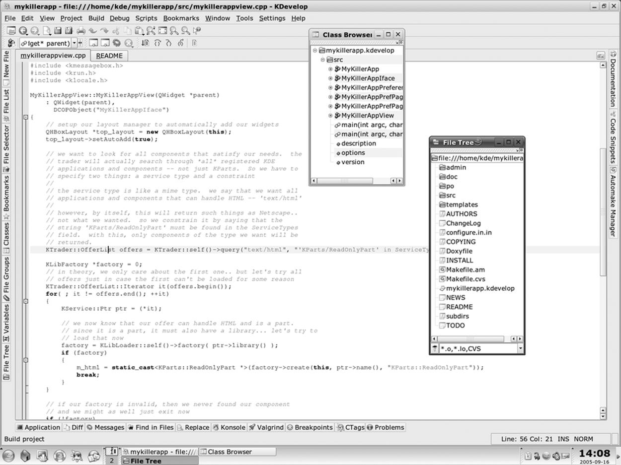
Figure 21-2. The KDevelop IDE
Emacs and XEmacs, by the way, make for very fine IDEs that integrate many additional tools such as gdb, as shown earlier in this chapter.
[*] We can't understand why it can be more difficult to type in a gcc command than to select a menu item from a menu, but then again, this might be due to our socialization.