Marketing Analytics: Data-Driven Techniques with Microsoft Excel (2014)

Part XI. Internet and Social Marketing

Chapter 43. The Mathematics Behind The Tipping Point

Malcolm Gladwell's book The Tipping Point (Back Bay Books, 2000) has sold nearly 3 million copies. In his book Gladwell explains how little things can have a large effect on determining whether a new product succeeds or fails in the marketplace. This chapter builds on the discussion of networks in Chapter 42, “Networks,” and examines two mathematical models that illuminate some of Gladwell's key ideas.

· You begin with an explanation of the classical theory of network contagion, which enables you to determine whether all nodes in a network eventually get turned on. The contagion model enables you to see how little things do indeed make a difference in the spread of a new product.

· You then modify the Bass model of product diffusion discussed in Chapter 27, “The Bass Diffusion Model,” to further illustrate some of Gladwell's main ideas.

Network Contagion

Marketing analysts want to know how knowledge of networks can help spread knowledge of their product. Consider the metaphor that each person who might buy a product is a node in a network. When the product first comes out, all nodes are in the “off” position corresponding to nobody having knowledge of the product. If you define the “on” position for a node as denoting that a person has knowledge of the product, then the marketer's goal is to turn all nodes on as quickly as possible.

Now reconsider the 10-node ring network with two links per node discussed in Chapter 42. Figure 43.1 shows this network.

Figure 43-1: 10-Node Network with two nodes per link

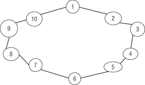
Suppose at present only Person 1 knows about your product. Call a person who knows about the product an on node and a person who does not know about the product an off node. To model the spread of a product (or disease!) the contagion model assumes there is a Threshold level (call it T) between 0 and 1 such that an off node can switch to on if at least a fraction T of a node's neighbors are on. Assume T = 0.5. Then the following sequence of events can ensue:

· Round 1: Nodes 2 and 10 turn on.

· Round 2: Nodes 3 and 9 turn on.

· Round 3: Nodes 4 and 8 turn on.

· Round 4: Nodes 5 and 7 turn on.

· Round 5: Node 6 turns on.

Even though you began with only one person knowing about the product, quickly everyone learned about it.

Now assume instead that T = 0.51. In Round 1 Nodes 2 and 10 are the only candidates to turn on. Node 2 has only 50 percent of its neighbors on, so Node 2 does not turn on. The same is true of Node 10. Therefore none of the other nine nodes will ever turn on. This example shows how a small increase in the threshold can make a big difference in who knows about the product. As Gladwell says, “Little things can make a big difference.”

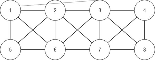
Now try and figure out who eventually will know about the product for the network in Figure 43.2 if T = 0.50 and originally only Node 2 is on. On nodes are shaded in subsequent figures.

· Round 1: 50 percent of Node 1 neighbors are on (Node 2 is on and Node 6 is off), so Node 1 turns on. Also 50 percent of Node 5 neighbors (Node 2 is on and Node 6 is off) are on, so Node 5 turns on. Node 3 does not turn on because only one of five neighbors is on. Node 7 has one of five neighbors on, so it does not turn on. None of Node 4's, Node 6's, or Node 8's neighbors are on, so none turn on. After Round 1 the network looks like Figure 43.3. (On nodes are shaded.)

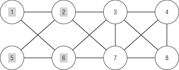
· Round 2: Two out of four neighbors of Node 6 are on, so Node 6 turns on. Node 3 has one of five neighbors on, so Node 3 does not turn on. Nodes 4 and 8 do not have neighbors on, so neither turns on. Node 7 has one of five neighbors turned on, so Node 7 remains off. The network now looks like Figure 43.4.

· Round 3: Node 3 has two of five neighbors on, so Node 3 stays off. Nodes 4 and 8 have no neighbors on, so they remain off. For Node 7, two out of five neighbors (or 40 percent) are on, so Node 7 stays off. At this point Nodes 3, 4, 7, and 8 never turn on.

Figure 43-2: Node 2 is initially on

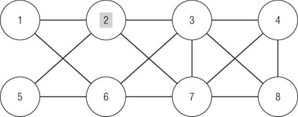
Figure 43-3: Round 1: Nodes 1, 2, and 5 are on

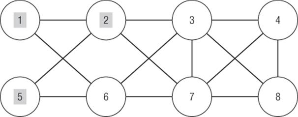
Figure 43-4: Round 2: Nodes 1, 2, 5, and 6 are on

This simple example can be tied to some of Gladwell's key ideas:

· Connectors (see pages 38–46 of The Tipping Point) who know a lot of people can be the key for a product managing to break out. For example, suppose Node 1 was more connected (say linked to Node 3 and Node 5) and Node 2 was also connected to Node 6. Also suppose T = 0.5 and Nodes 1 and 2 are initially on. You can verify (see Exercise 1) that all nodes in the network shown in Figure 43.5 eventually turn on due to the increased influence of the connectors: Nodes 1 and 2. Gladwell's classic example of a connector was Paul Revere spreading the word that “The British are coming.” William Dawes also tried to spread the word, but Revere was better connected, so he was much more successful in spreading the word. The lesson for marketers is that well-connected customers (such as people with high betweenness centrality) can make the difference between a successful and failed product rollout.

· Gladwell also discusses the importance (see pages 54–55) of weak ties in spreading knowledge of a product. Recall from Chapter 42 that in the Strogatz-Watts Small World model the average distance between nodes in a network can be greatly reduced by introducing a few weak ties that correspond to arcs that connect people who (without the weak ties) are far apart in the network. Many products (such as the Buick Rendezvous in the early 2000s) try hard to spread the word about products in Times Square because people in Times Square are often connectors who are not from New York City and have weak ties to people from far-flung areas of the United States and the rest of the world.

· Mavens (see pages 59–68) are people who are knowledgeable and highly persuasive about a product. In effect mavens reduce the threshold T. You can see (Exercise 2) that all nodes in the network of Figure 43.2 would turn on eventually if you could lower T to 0.4.

· Great salespeople (see pages 78–87) can make the difference between a successful and failed product rollout. A great salesperson reduces T because she makes the potential customer less resistant to trying a new product.

Figure 43-5: All nodes turn on

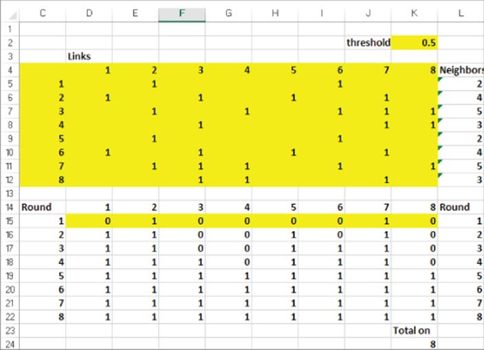
For an arbitrary 8-node network, the Contagion.xlsx file enables you to vary T, the links in the network, and the nodes that begin on and trace the path of nodes turning on. Define a node that is initially on as a seeded node. As shown in Figure 43.6, you enter a 1 in the range D5:K12 for each arc in the network. Also enter T in cell K2 and the initial on nodes are indicated by a 1 in the range D15:K15. As shown in K24 of the Initial Seeding worksheet, only four nodes eventually turn on. In the Seed 2 nodes worksheet (see Figure 43.7) you can see that if the firm seeded Node 7 as well as Node 2, you could eventually turn the whole market on. This example shows it might pay to give away your product to members of difficult-to-reach market segments.

Figure 43-6: Only four nodes turn on when you start with Node 2

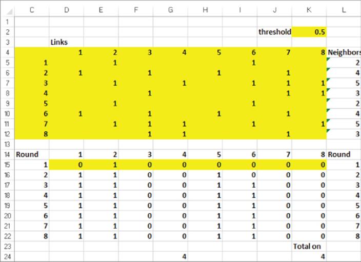
Figure 43-7: Nodes 2 and 7 on cause all nodes to turn on

A Bass Version of the Tipping Point

On pages 12 and 13 of his book Gladwell gives several examples of the tipping point concept, including the following:

· When the fraction of African-Americans in a neighborhood exceeds 20 percent, most remaining whites suddenly leave the neighborhood.

· Teenage pregnancy rates in neighborhoods with between 5 and 40 percent professional workers are relatively constant, but in neighborhoods with 3.2 percent professionals, pregnancy rates double.

Essentially the central thesis of The Tipping Point is that in many situations involving social decision making there exists a threshold value (call the threshold p*) for a key parameter (call the parameter p) such that small movements of the parameter around p* can elicit a huge response. In the first example p = the fraction of African-Americans and when p > p* = 0.20 a huge social response (more whites moving out) is elicited. In the second example p = fraction of professional workers in the neighborhood and for p < p* = 0.05 a huge social response (more teenage pregnancies) is elicited.

The idea of a threshold is easily understood if you consider every individual in a population to be either sick or healthy. Let p = probability that a contact between a sick person and a healthy person infects the healthy person. In this context the tipping point corresponds to the existence of a threshold value p* such that a small increase of p above p* elicits a large increase in the number of people who eventually become sick. You can use your knowledge of the Bass diffusion model (see Chapter 27) to analyze this situation. This model demonstrates that a small change in p can result in a large change in the number of people who eventually get infected. The model is in the basstippoint.xlsx file (see Figure 43.8). The evolution of the number of infected and healthy people at time t = 0, 1, 2, …, 100 is described here:

1. Assume there is a total of 1,000 people (enter this in E3), and at Time 0 nobody has been sick.

2. In cell E1 enter the probability (0.0013) that a contact between a sick and healthy person will infect the healthy person.

3. In cell E2 enter the probability (0.2) that a sick person gets better during a period. This implies that a person is sick for an average of 5 days. When a sick person gets better, he cannot ever infect anyone. This corresponds in the marketing context to a person “forgetting” about a product and not spreading the word about the product.

4. At Time 1 assume 1 person is sick. In cell D7 compute the number of people who will get better at Time 1 with the formula =C7*get_better.

5. Copy this formula to the range D8:D106 to compute the number of people who get better during each of the remaining periods.

6. In cell E7 use the formula =C7*G6 to compute the number of contacts for t = 1 between sick people and people who have never been sick. This formula is analogous to the Bass model formula that models the word-of-mouth term by multiplying those people who have purchased the product times those who have not.

7. Copy this formula to the range E8:E106 to compute the number of contacts between sick people and people who are never sick during the remaining periods.

8. In cell F7 use the formula =infect*E7 to compute the number of contacts for t = 1 that result in infection.

9. Copy this formula to the range F8:F106 to determine the number of new infections during the remaining periods.

10. In cell G7 use the formula =MAX(G6-F7,0) to reduce the number of people who have never been sick by the number of infections at t = 1. This yields the number of people who have not been sick by the end of period 1.

11. Copy this formula to the range G8:G106 to compute for t = 2, 3, …, 100 the number of people who are not sick by the end of period t. Using the max function ensures that the number of people who are not sick will stop at 0 when everyone has become sick.

Figure 43-8: Bass Tipping Point model

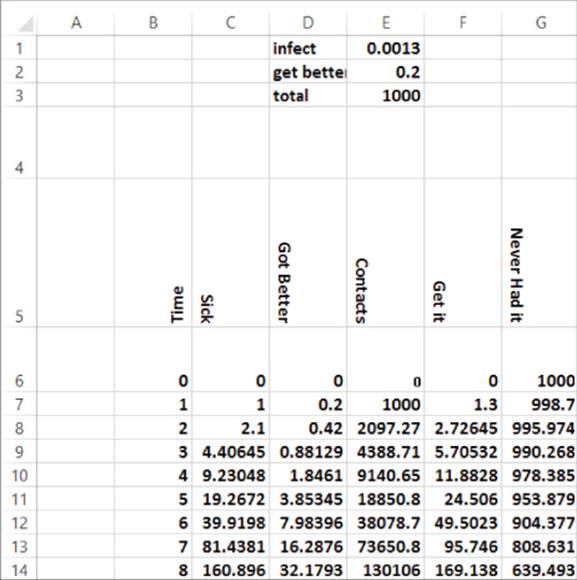
Figure 43.9 shows a two-way data table with row input cell = probability of getting better; column input cell = probability of infection; and output cell =Total–G107, which measures the number of people who have become sick by t =100.

Figure 43-9: Data table summarizing number of people who eventually get sick

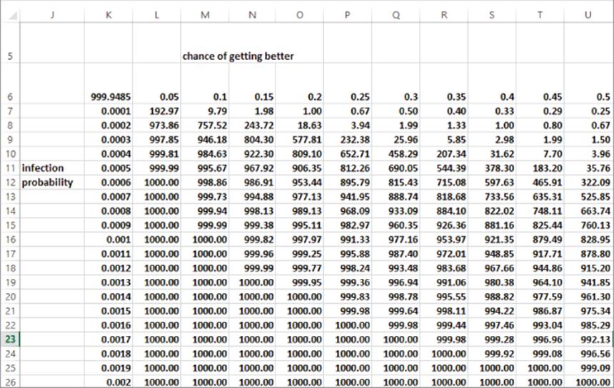
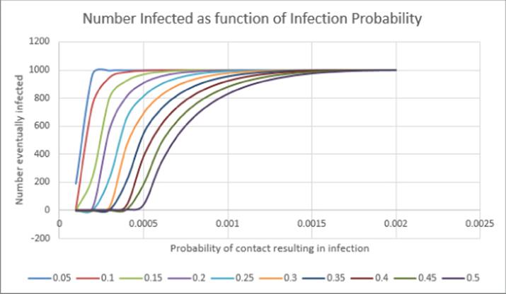
As expected, an increase in the chance of getting better decreases the number of people who eventually get sick. This is because an increase in the chance of getting better means a sick person has less time to infect healthy people. An increase in the chance of infection increases the number of people who eventually get sick. Also the infection probability needed to infect everyone increases as the chance of getting better increases. This is reasonable because if people are “carriers” for less time, you need a more virulent disease to ensure that everyone is infected. Figure 43.10 summarizes the data table by graphing for each probability of getting better the dependence of the number of people who eventually fall ill on the chance of infection. For each curve there is a steep portion that indicates the tipping point for the infection probability. For example, if there is a 50-percent chance of a healthy person getting better, the tipping point appears to occur when the probability of a contact between a healthy and sick person resulting in a new sick person reaches a number between 0.005 and 0.006.

Figure 43-10: Number infected as a function of infection probability

The marketing analog of the epidemic model is clear: to be infected is to know about a product and to become healthy means you are no longer discussing the product. After recognizing that the marketer's goal is to “infect” everyone, this model provides two important marketing insights:

· Lengthening the amount of time that people talk about your product (decreasing chance of becoming healthy) can enhance the spread of your product.

· Sometimes, a small increase in the persuasiveness of people who discuss your product or a small decrease in product resistance to your product among noncustomers can greatly increase the eventual sales of your product.

Summary

In this chapter you learned the following:

· The contagion model assumes that a node will turn on if at least a fraction T of a node's neighbors is already on.

· A small difference in T or the number of initial on nodes can make a huge difference in the eventual number of on nodes.

· Connectors, mavens, and salespeople can provide the extra energy needed for a product to achieve 100-percent market penetration.

· The Bass version of Gladwell's tipping point model implies that lengthening the amount of time that people talk about your product (decreasing chance of becoming healthy) can enhance the spread of your product. Also a small increase in the persuasiveness of people who discuss your product or a small decrease in product resistance to your product among noncustomers may greatly increase the eventual sales of your product.

Exercises

1. Consider a network on a circle for which each node is linked to the closest four nodes. Suppose Node 1 in currently on. If T = 0.5, which nodes will eventually turn on? If T = 0.3, which nodes will eventually turn on?

2. For the network in Figure 43.2, assume that T = 0.4 and Node 2 is initially on. Show that all nodes will eventually turn on.

3. Modify the network in Figure 43.2 so that Node 1 is now also linked to Node 3 and Node 5; and Node 2 is now also linked to Node 6. Assume that T = 0.5 and Nodes 1 and 2 are initially on. Verify that if Node 2 is initially on and T = 0.5 that all nodes will eventually turn on.