Marketing Analytics: Data-Driven Techniques with Microsoft Excel (2014)
Part XI. Internet and Social Marketing
Chapter 44. Viral Marketing
On July 14, 2010, Old Spice launched a viral video campaign (see www.youtube.com/watch?v=owGykVbfgUE) involving ex-San Francisco linebacker Isaiah Mustafa. This video received 6.7 million views after 24 hours and 23 million views after 36 hours. Likewise, the famous “Gangnam Style” (www.youtube.com/watch?v=9bZkp7q19f0) video has now received nearly 2 billion views! Because views of these videos spread quickly like an epidemic, the study of such successes is often referred to as viral marketing. Of course, many videos are posted to YouTube (like the author's video on Monte Carlo simulation) and receive few views. This chapter discusses two mathematical models of viral marketing that attempt to model the dynamics that cause a video to either go viral or die a quick death.
For simplicity this chapter assumes that the viral campaign is a video and you want to describe the viewing history of the video. The two mathematical models attempt to explain how the number of people viewing a video grows over time. Assume at the beginning of the first period (t = 1), Npeople view the video.
· The first model (Watts' Model) is based on Duncan Watts' 2007 article “The Accidental Influentials” (Harvard Business Review, Vol. 85, No. 2, 2007, pp. 22–23). This model provides a simple explanation for the spread of a video, but as you will see, Watts ignores the fact that several people may send the video on to the same person. Watts' Model predicts the total views of a video based on two parameters: N = initial number of people who view the video and R = the expected number of new viewers generated by a person who has just seen the video.
· The second model improves on Watts' Model by including the fact that some of the videos sent on at a given time will be sent to the same person.
Watts' Model
Watts assumes that at the beginning of the first period (t = 1) the maker of the video “seeds” the video by getting N people to view it. Then during each time period, each new viewer is assumed to pass the video on to R new viewers. This implies that at t = 2, NR new viewers are generated; at time t = 3, NR(NR) = NR2 new viewers are generated; at t = 4, (NR2) * NR = NR3 new viewers are generated; and so on. This implies that there will be a total of S distinct viewers of the video where Equation 1 is true:
1 ![]()
If R>=1, S will be infinite, indicating a “viral” video. Of course, R cannot stay greater than 1 forever, so in all likelihood R will drop after a while.
Assuming that R stays constant at a value less than 1, you may evaluate S by using an old trick from high school algebra. Simply multiply Equation 1 by R, obtaining Equation 2:
2 ![]()
Subtracting Equation 2 from Equation 1 yields S-RS = N. Solving for S you find Equation 3:
3 ![]()
In many situations you know S and N, so you may use Equation 3 to solve for R and find R = (S-N)/S.
Watts' Model can be used with many examples of viral marketing campaigns. Listed here are a few for which Watts listed the relevant model parameters:
· Tom's Petition was a 2004 petition for gun control. This petition had R = 0.58 and N = 22,582.
· Proctor and Gamble started a campaign to promote Tide Coldwater as an energy-efficient detergent. This campaign began with N near 900,000 and R = 0.041.
· The Oxygen Network ran a campaign to raise money for Hurricane Katrina, which had N = 7,064, S = 30,608, and an amazingly large R = 0.769.
Watts' Model shows that the initial seeding (N) and the number of new viewers (R) are both critical to determining the final number of video views. Watts' Model assumes, however, that each person reached at, say, time t has never been reached before. This is unreasonable. For example, suppose there is a population of 1,000,000 people, and at the beginning of time t 800,000 people have seen the video. Then it seems highly unlikely that the NRt-1 new viewers the Watts Model generates at Time t are all people who have not already seen the video. Also if R >= 1, Watts predicts an infinite number of people will see the video, and this does not make sense. In the next section you modify, the Watts Model in an attempt to resolve these issues.
A More Complex Viral Marketing Model
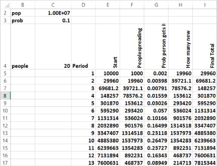
A revised version of Watts' Model is in the worksheet basic of the workbook viral.xlsx (see Figure 44.1). The model requires the following inputs:
· The population size N (named as pop and entered in C2). Assume that a maximum of 10 million people might see the video. Note that 1.00 + E + 07 is scientific notation and is equivalent to 1*107 = 10,000,000.
· The probability (given range name prob entered in C3) that a person who sees the video will send the video on to at least one person. Assume this probability is 0.1. Assume that everyone who is sent the video views the video. In Exercise 6, you modify this assumption.
· If the video is sent on, the average number of people (given the range name of people entered in C4) to whom a person will send the video. Assume that on average a person will send the video to 20 people. Note that Watts' R = prob * people. In this case R = (0.1) * 20 = 2. In this case Watts' Model would predict an infinite number of people to see the video. As you will see the model predicts that 7,965,382 of the 10,000,000 potential viewers will eventually see the video.
· In cell E5 enter the number of people who are “seeded” as video viewers at the beginning of Period 1. Assume 10,000 viewers are seeded.
Figure 44-1: Improved viral marketing model
During each period t, the model tracks the following quantities:
· At the start of period t, the number of people who have seen the video
· The number of people who were newly introduced to the video during period t – 1 and are potential spreaders of the video during period t
· The probability that a given person will receive the video during period t. Estimating this probability requires some discussion of the binomial and Poisson random variables.
· The number of new viewers of the video who are created during period t
· The number of people who have viewed the video by the end of period t
· Assume 400 time periods
Before explaining the formulas that underlie the model, you need to briefly consider the binomial and Poisson random variables.
The Binomial and Poisson Random Variables
The binomial random variable is used to compute probabilities in the following situation:
· N repeated trials occur in which each trial results in success or failure.
· The probability of success on each trial is P.
· The trials are independent, that is, whether a given trial results in a success or failure has no effect on the result of the other N-1 trials.
· The Excel BINOMDIST function can be used to compute binomial probabilities in the following situations:
· Entering the formula =BINOMDIST(x, N, P, 1) in a cell computes the probability of <=x successes in N trials.
· Entering the formula =BINOMDIST(x, N, P, 0) in a cell computes the probability of exactly x successes in N trials.
· The mean of a binomial random variable is simply N*P.
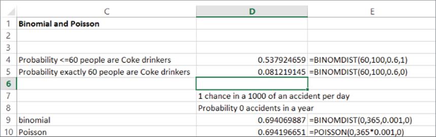
The file BinomialandPoisson.xlsx (see Figure 44.2) illustrates the computation of binomial probabilities. Assume that 60 percent of all people are Coke drinkers and 40 percent are Pepsi drinkers. Define a success such that a person is a Coke drinker. In cell D4 you can use the formula=BINOMDIST(60,100,0.6,1) to compute the probability (53.8 percent) that <= 60 people in a group of 100 are Coke drinkers. In cell D5 you can use the formula =BINOMDIST(60,100,0.6,0) to compute the probability (8.1 percent) that exactly 60 people are Coke drinkers.
Figure 44-2: Illustration of binomial and Poisson probabilities
The Poisson random variable is a discrete random variable that can assume the values 0, 1, 2, …. To determine the probability that a Poisson random variable assumes a given value, all you need is the mean (call it M) of the Poisson random variable. Then the following Excel formulas can be used to compute Poisson probabilities:
· POISSON(x, M, 1) gives the probability that the value of a Poisson random variable with mean M is ≤ x.
· POISSON(x, M, 0) gives the probability that the value of a Poisson random variable with mean M = x.
The Poisson random variable is relevant in many interesting situations (particularly in queuing or waiting line models), but for your purposes, use the fact that when N is large and P is small, binomial probabilities can be well approximated by Poisson probabilities where M = NP. To illustrate this idea, assume that a teen driver has a 0.001 chance of having an accident each day. What is the chance the teen will have 0 accidents in a year? Here define a “success” on a day to be an accident. You have N = 365 and P =0.001. In cell D9 the formula =BINOMDIST(0,365,0.001,0) computes the chance of 0 accidents (69.41 percent) in a year. Now the mean number of accidents in a year is 0.001(365) = 0.365, so using the Poisson approximation to the binomial, you can estimate the probability of 0 accidents in a year with the formula = POISSON(0,365*0.001,0). You obtain 69.42 percent, which is an accurate approximation.
Building the Model of Viral Marketing
Armed with your knowledge of the binomial and Poisson random variables, you are now ready to explain how your model estimates the ultimate penetration level for a viral video.
In Period 1, 10 percent of the 10,000 people will spread the product. This number is computed in cell F5 with the formula =prob*E5.
Now comes the hard part! Of the 10,000 people who have seen the video in Period 1, (.10)*10,000 = 1,000 of them will pass it on. Each of these 1,000 people sends the video to an average of 20 people, so 20,000 e-mails or text messages describing the video will be sent during Period 1. This does not mean (as Watts assumes) that 20,000 new people see the video. This is because it is possible that a single person will receive e-mails or texts about the video from several different people.
Now estimate the probability that a person will receive a video during Period 1. For a given person there is a chance 1/pop that each of the 20,000 e-mails or texts sent out during Period 1 will go to the person. Thus on average a person receives 20,000/pop e-mails during Period 1, and the chance that the person receives 0 e-mails can be approximated by = POISSON(0,F5people/pop,TRUE), and the probability that a person will receive at least 1 e-mail during Period 1 is in cell G5 with the formula =1-POISSON(0,F5people/pop,TRUE).
The following steps allow you to trace the evolution of the number of people who have seen the video:
1. Multiply the number of people who have not yet seen the video (pop – G5) times 0.0002 to compute the number of new Period 1 video viewers. The formula =(pop-E5)*G5 computes the number (1,997.8) of new viewers of the video during Period 1.
2. In cell I5 use the formula =E5+H5 to add the 1,997.8 new viewers to the original 10,000 viewers to obtain the number of total viewers of the video (11,997.8) by the end of Period 1.
3. Copy the formula =I5 from E6 to E7:E404 to compute the number of total viewers at the beginning of the period by simply copying the ending viewers from the previous period.
4. Copy the formula =H5 from F6 to F7:F404 to list the number of people available to spread the video during each period. This number is simply the number of new viewers during the previous period.
5. Copy the formula =1-POISSON(0,F6*prob*people/pop,TRUE) from G6 to G7:G404 to apply the Poisson approximation to the binomial to compute the probability that a person who has not already seen the video will be sent the video during the current period.
6. Copy the formula =(pop-E5)*G5 from H5 to H6:H404 to compute for each period the number of new viewers of the video by multiplying the number of people who have not seen the video times the chance that each person sees the video.
7. Copy the formula =E5+H5 from I5 to I6:I404 to compute the total number of viewers to date of the video by adding previous viewers to the new viewers created during the current period.
It is estimated that 7,971,541 people will eventually see the video.
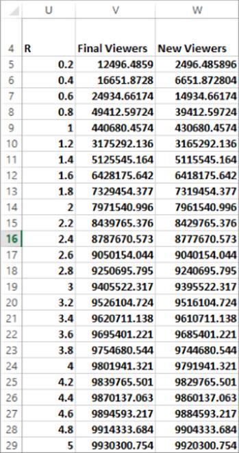
Using a Data Table to Vary R
In your new viral marketing model, prob and People impact the predicted spread of the video only through their product prob * People, which is the expected number of people to whom each new video viewer passes the video. Watts set prob * People = R. The worksheet data table of the workbook viral.xlsx varied R. Figure 44.3 shows the dependence of the final viewers on R. Note that until R exceeds 1 the video does not go viral. For example, when R = 0.8, only 49,413 people eventually see the video while if R = 2 nearly 8 million people see the video.
Figure 44-3: Dependence of video spread on R
Summary
In this chapter you learned the following:
· Let N = initial viewers of a video and R = new viewers generated per person by a video. Then for R>1, the Watts' Model predicts the eventual number of viewers will be infinite, and for R<1, the Watts' Model predicts the video will eventually reach N/(1-R) viewers.
· Because an infinite number of viewers is impossible, the Watts' Model is flawed. The major flaw is that many people may send the video to the same person. The more complex model (which utilizes the Poisson approximation to the binomial random variable) resolves this problem.
Exercises
1. Verify that for the Oxygen Network the values of N = 7,064 and S = 30,608 imply that R = 0.769.
2. Using the Watts' Model estimate the number of new viewers generated by the Coldwater Tide campaign. Use N = 900,000 and R = 0.041.
3. Apply your new viral marketing model to the Tide Coldwater campaign.
4. Determine the dependence of the spread of the video on the population size as the population size varies between 10 and 100 million.
5. For the Watts' Model estimate the final number of viewers for Tom's Petition. This petition had R = 0.58 and N = 22,582.
6. Suppose a fraction F<1 of people receiving your video view it, but a fraction 1-F do not look at the video. How does this modify the Watts' Model?
All materials on the site are licensed Creative Commons Attribution-Sharealike 3.0 Unported CC BY-SA 3.0 & GNU Free Documentation License (GFDL)
If you are the copyright holder of any material contained on our site and intend to remove it, please contact our site administrator for approval.
© 2016-2026 All site design rights belong to S.Y.A.