Marketing Analytics: Data-Driven Techniques with Microsoft Excel (2014)

Part XI. Internet and Social Marketing

Chapter 45. Text Mining

Every day Twitter handles more than 400 million tweets. Miley Cyrus' 2013 VMA fiasco generated more than 17 million tweets! Many of these tweets comment on products, TV shows, or ads. These tweets contain a great deal of information that is valuable to marketers. For example, if you read every tweet on a Super Bowl ad, you could determine if the United States liked or hated the ad. Of course, it is impractical to read every tweet that discusses a Super Bowl ad. What is needed is a method to find all tweets and then derive some marketing insights from the tweets. Text mining refers to the process of using statistical methods to glean useful information from unstructured text. In addition to analyzing tweets, you can use text mining to analyze Facebook and blog posts, movies, TV, and restaurant reviews, and newspaper articles. The data sets from which text mining can glean meaningful insights are virtually endless. In this chapter you gain some basic insights into the methods you can use to glean meaning from unstructured text. You also learn about some amazing applications of text mining.

In all of the book's previous analysis of data, each data set was organized so that each row represented an observation (such as data on sales, price, and advertising during a month) and each column represented a variable of interest (sales each month, price each month, or advertising each month). One of the big challenges in text mining is to take an unstructured piece of text such as a tweet, newspaper article, or blog post and transform its contents into a spreadsheet-like format. This chapter begins by exploring some simple ways to transform text into a spreadsheet-like format. After the text has been given some structure, you may apply many techniques discussed earlier (such as Naive Bayes, neural networks, logistic regression, multiple regression, discriminant analysis, principal components, and cluster analysis) to analyze the text. The chapter concludes with a discussion of several important and interesting applications of text mining including the following:

·        Using text content of a review to predict whether a movie review was positive or negative

·        Using tweets to determine whether customers are happy with airline service

·        Using tweets to predict movie revenues

·        Using tweets to predict if the stock market will go up or down

·        Using tweets to evaluate viewer reaction to Super Bowl ads

Text Mining Definitions

Before you can understand any text mining studies, you need to master a few simple definitions:

·        A corpus is the relevant collection of documents. For example, if you want to evaluate the effectiveness of a Sofia Vergara Diet Pepsi ad, the corpus might consist of all tweets containing references to Sofia Vergara and Diet Pepsi.

·        A document consists of a list of individual words known as tokens. For example, for the tweet “Love Sofia in that Diet Pepsi ad,” it would contain seven tokens.

·        In a tweet about advertising, the words “ad” and “ads” should be treated as the same token. Stemming is the process of combining related tokens into a single token. Therefore “ad” and “ads” might be grouped together as one token: “ad.”

·        Words such as “the,” appear often in text. These common words are referred to as stopwords. Stopwords give little insight into the meaning of a piece of text and slow down the processing time. Therefore, stopwords are removed. This process is known as stopping. In the Sofia Vergara tweet, stopping would remove the words “in” and “that.”

·        Sentiment analysis is an attempt to develop algorithms that can automatically classify the attitude of the text as pro or con with respect to a topic. For example, sentiment analysis has been used in attempts to mechanically classify movie and restaurant reviews as favorable or unfavorable.

Giving Structure to Unstructured Text

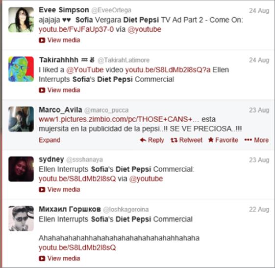
To illustrate how you can give structure to unstructured text, again consider the problem of analyzing tweets concerning Sofia Vergara in Diet Pepsi ads. To begin you need to use a statistical package with text mining capabilities (such as R, SAS, SPSS, or STATISTICA) that can interface with Twitter and retrieve all tweets that are relevant. Pulling relevant tweets is not as easy as you might think. You might pull all tweets containing the tokens Sofia, Vergara, Diet, and Pepsi, but then you would be missing tweets such as those shown in Figure 45.1, which contain the token Sofia and not Vergara.

Figure 45-1: Tweets on Sofia Vergara Diet Pepsi ad

As you can see, extracting the relevant text documents is not a trivial matter. To illustrate how text mining can give structure to text, you can use the following guidelines to set the stage for an example:

·        Assume the corpus consists of N documents.

·        After all documents undergo stemming and stopping, assume a total of W words occur in the corpus.

·        After stemming and stopping is concluded for i = 1, 2, …,W and j = 1, 2, …, N, let Fij = number of times word i is included in document j.

·        For j = 1, 2, …, W define Dj = number of documents containing word j.

After the corpus of relevant tweets has undergone stemming and stopping, you must create a vector representation for each document that associates a value with each of the W words occurring in the corpus. The three most common vector codings are binary coding, frequency coding, and theterm frequency/inverse document frequency score (tf-idf for short). The three forms of coding are defined as follows:

NOTE

Before coding each document, infrequently occurring words are often deleted.

·        The binary coding simply records whether a word is present in a document. Therefore, the binary representation for the ith word in the jth document is 1 if the ith word occurs in the jth document and is 0 if the ith word does not occur in the jth document.

·        The frequency coding simply counts for the ith word in the jth document the number of times (Fij) the ith word occurs in the jth document.

·               To motivate the term frequency/inverse document frequency score, suppose the words cat and dog each appear 10 times in a document. Assume the corpus consists of 100 documents, and 50 documents contain the word cat and only 10 documents contain the word dog. Despite each appearing 10 times in a document, the occurrences of dog in the document should be given more weight than the occurrences of cat because dog appears less frequently in the corpus. This is because the relative rarity of dog in the corpus makes each occurrence of dog more important than an occurrence of cat. After defining Tj = number of tokens in document j, you can define the following equation:

1 

The term Fij / Tj is the relative frequency of word i in document j, whereas the term log(N / Dj) is a decreasing function of the number of documents in which the word i occurs.

These definitions can be illustrated by considering a corpus consisting of the following three statements about Peyton Manning (see Figure 45.2 and the Text mining coding.xlsx) file.

·        Document 1: Peyton Manning is a great quarterback.

·        Document 2: Peyton is a great passer and has a great offensive line.

·        Document 3: Peyton is the most overrated of all quarterbacks.

Figure 45-2: Examples of text mining coding

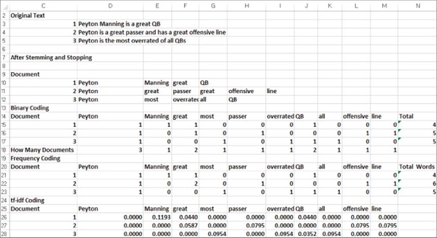
After stemming and stopping is performed, the documents are transformed into the text shown in rows 10–12. Now you can work through the three vector codings of the text.

Binary Coding

Rows 15–17 show the binary coding of the three documents. You simply assign a 1 if a word occurs in a document and a 0 if a word does not appear in a document. For example, cell F16 contains a 1 because Document 2 contains the word great, and cell G16 contains a 0 because Document 2 does not contain the word most.

Frequency Coding

Rows 21–23 show the frequency coding of the three documents. You simply count the number of times the word appears in the document. For example, the word great appears twice in Document 2, so you can enter a 2 in cell F22. Because the word “most” does not occur in Document 2, you enter a 0 in cell G22.

Frequency/Inverse Document Frequency Score Coding

Copying the formula =(D21/$N21)*LOG(3/D$18) from D26 to the range D26:M28 implements Equation 1. In this formula D21 represents Fij; $N21 represents the number of words in the document; 3 is the number of documents in the corpus; and D$18 is the number of documents containing the relevant word. Note that the use of dollar signs ensures that when the formula is copied the number of words in each document and the number of documents containing the relevant word are pulled from the correct cell. The tf-idf coding attaches more significance to “overrated” and “all” in Document 3 than to “great” in Document 2 because “great” appears in more documents than “overrated” and “all.”

Applying Text Mining in Real Life Scenarios

Now that you know how to give structure to a text document, you are ready to learn how to apply many tools developed earlier in the book to some exciting text mining applications. This section provides several examples of how text mining can be used to analyze documents and make predictions in a variety of situations.

Text Mining and Movie Reviews

In their article “Thumbs up? Sentiment Classification using Machine Learning Techniques” (Proceedings of EMNNP, 2002, pp. 79–86) Pang, Lee, and Vaithyanathan of Cornell and IBM applied Naive Bayes (see Chapter 39, “Classification Algorithms: Naive Bayes Classifier and Discriminant Analysis”) and other techniques to 2,053 movie reviews in an attempt to use text content of a review as the input into mechanical classification of a review as positive or negative.

The authors went about this process by first converting the number of stars a reviewer gave the movie to a positive, negative, or neutral rating. They then applied frequency and binary coding to each review. You would expect that reviews containing words such as brilliant, dazzling, and excellent would be favorable, whereas reviews that contained words such as bad, stupid, and boring would be negative.

They also used Naive Bayes (see Chapter 39) based on binary coding in an attempt to classify each review, in terms of the Chapter 39 notation C1 = Positive Review, C2 = Negative Review, and C3 = Neutral review. The n attributes X1, X2, …., Xn correspond to whether a given word is present in the review. For example, if X1 represents the word brilliant, then you would expect P(C1 | X1 = 1) to be large and P(C2 | X1 = 1) to be small.

The authors then used machine learning (a generalization of the neural networks used in Chapter 15, “Using Neural Networks to Forecast Sales”) to classify each review using the frequency coding.

Surprisingly, the authors found that the simple Naive Bayes approach correctly classified 81 percent of all reviews, whereas the more sophisticated machine learning approach did only marginally better than Naive Bayes with an 82-percent correct classification rate.

Sentiment Analysis of Airline Tweets

Jeffrey Breen of Cambridge Aviation Research (see pages 133–150 of Practical Text Mining, by Elder et. al, 2012, Academic Press) collected thousands of tweets that commented on airline service. Breen simply classified a tweet as positive or negative by counting the number of words associated with a positive sentiment and number of words associated with negative sentiments (for a sample list of positive and negative words, see http://www.wjh.harvard.edu/˜inquirer/Positiv.html and http://www.wjh.harvard.edu/˜inquirer/Negativ.html.

A tweet was classified as positive if the following was true:

Number of Positive Words – Number of Negative Words >= 2

The tweet was classified as negative if the following was true:

Number of Positive Words – Number of Negative Words <= -2

Breen found that that JetBlue (84-percent positive tweets) and Southwest (74-percent positive tweets) performed best. When Breen correlated each airline's score with the national survey evaluation of airline service conducted by the American Consumer Satisfaction Index (ACSI) he found an amazing 0.90 correlation between the percentage of positive tweets for each airline and the airline's ACSI score. Because tweets can easily be monitored in real time, an airline can track over time the percentage of positive tweets and quickly see whether its service quality improves or declines.

Using Twitter to Predict Movie Revenues

Asu and Huberman of HP Labs used tweets to create accurate predictions of movie revenues in their article, “Predicting the Future with Social Media” submitted in 2010 (see the PDF at www.hpl.hp.com/research/scl/papers/socialmedia/socialmedia.pdf).

For 24 movies the authors used the number of tweets each day in the 7 days before release and the number of theaters in which the movie opened to predict each movie's opening weekend revenues. They simply ran a multiple regression (see Chapter 10, “Using Multiple Regression to Forecast Sales”) to predict opening weekend revenue from the aforementioned independent variables. Their regression yielded an adjusted R2 value of 97.3 percent. Adjusted R2 adjusts the R2 value discussed in Chapter 10 for the number of independent variables used in the regression. If a relatively unimportant independent variable is added to a regression, then R2 never decreases, but adjusted R2 decreases. Formally adjusted R2 may be computed as:

1 − (1 − R2)*(n − 1) / (n − k − 1),

where n = number of observations and k = number of independent variables.

The authors compared their predictions to predictions from the Hollywood Stock Exchange (www.hsx.com/). HSX is a prediction market in which buyers and sellers trade based on predictions for a movie's total and opening weekend revenues. Using the HSX prediction and number of theaters as independent variables, a multiple regression yielded an adjusted R2 value of 96.5 percent of the variation in opening weekend revenues. Therefore, the author's use of tweets to predict opening weekend movie revenues outperformed the highly regarded HSX predictions.

In trying to predict a movie's revenue during the second weekend, the authors applied sentiment analysis. They classified each tweet as positive, negative, or neutral. (See the paper for details of their methodology.) Then they defined the PNratio (Positive to Negative) as Number of Positive Tweets / Number of Negative Tweets. Using the tweet rates for the preceding seven days to predict second weekend revenues yielded an adjusted R2 of 0.84, whereas adding a PNratio as an independent variable increased the adjusted R2 to 0.94. As an example of how a large PNratio reflects favorable word of mouth, consider the movie The Blind Side, for which Sandra Bullock won a Best Actress Oscar. In the week before its release, this movie had a PNratio of 5.02, but after 1 week the movie's PNratio soared to 9.65. Amazingly, The Blind Side's second week revenues of $40 million greatly exceeded the movie's week 1 revenues of $34 million. Most movies experience a sharp drop-off in revenue during the second week, so The Blind Side illustrates the powerful effect that favorable word of mouth can have on future movie revenues.

Using Twitter to Predict the Stock Market

Bollen, Mao, and Zheng of Indiana University and the University of Manchester used the collective “mood” expressed by recent tweets to predict whether the Dow Jones Index would decrease or increase in their article, “Twitter Mood Predicts the stock market,” (Journal of Computational Science, Volume 2, 2011, pp. 1–8). They first used sentiment analysis to classify 9.8 million tweets as expressing a positive or negative mood about the economy. For Day t they defined PNt = ratio of positive to negative tweets and Dt = Dow Jones Index at end of day t − Dow Jones Index at end of day t − 1.

The authors tried to predict Dt using PNt-1, PNt-2, PNt-2, Dt-1, Dt-2, and Dt-3. Predictions from a neural network (See Chapter 15, “Using Neural Networks to Forecast Sales”) correctly predicted the direction of change in the Dow 84 percent of the time. This is truly amazing because the widely believed Efficient Market Hypothesis implies that the daily directional movement of a market index cannot be predicted with more than 50-percent accuracy.

Using Tweets to Evaluate Super Bowl Ads

In 2013 companies paid approximately $3 million dollars for a 30-second Super Bowl ad. Naturally, advertisers want to know if their ads are worthwhile. Professor Piyush Kumar of the University of Georgia analyzed more than one-million tweets that commented on Super Bowl 2011 ads. By performing sentiment analysis on the ads, Kumar found that the 2011 Bud Light ad (www.youtube.com/watch?v=I2AufnGmZ_U) was viewed as hilarious. Unfortunately for car manufacturers, only the Volkswagen ad http://www.youtube.com/watch?v=9H0xPWAtaa8 received a lot of tweets. The lack of tweets concerning other auto ads indicates that these ads made little impact on Super Bowl viewers.

Summary

In this chapter you learned the following:

·        To glean impact from the text, the text must be given structure through a vector representation that implements a coding based on the words present in the text.

·        Binary coding simply records whether a word is present in a document.

·        Frequency coding counts the number of times a word is present in a document.

·        The term-frequency/inverse document frequency score adjusts frequency coding of a word to reduce the significance of a word that appears in many documents.

·        After text is coded many techniques, such as Naive Bayes, neural networks, logistic regression, multiple regression, discriminant analysis, principal components, and cluster analysis, can be used to gain useful insights.

Exercises

1. Consider the following three snippets of text:

·        The rain in Spain falls mainly in the plain.

·        The Spanish World Cup team is awesome.

·        Spanish food is beyond awesome.

After stemming and stopping these snippets, complete the following tasks:

(a) Create binary coding for each snippet.

(b) Create frequency coding for each snippet.

(c) Create tf-idf coding for each snippet.

2. Use your favorite search engine to find the definition of “Amazon mechanical Turk.” If you were conducting a text mining study, how would you use Amazon mechanical Turks?

3. Describe how text mining could be used to mechanically classify restaurant reviews as favorable or unfavorable.

4. Describe how text mining could be used to determine from a member of Congress' tweets whether she is conservative or liberal.

5. Describe how text mining could be used to classify The New York Times stories as international news, political news, celebrity news, financial news, science and technology news, entertainment news, obituary, and sports news.

6. Alexander Hamilton, John Jay, and James Madison wrote The Federalist Papers, a series of 85 essays that provide reasons for ratifying the U.S. Constitution. The authorship of 73 of the papers is beyond dispute, but for the other 12 papers, the author is unknown. How can you use text mining in an attempt to determine the authorship of the 12 disputed Federalist Papers?

7. Suppose you are a brand manager for Lean Cuisine. How can use text mining of tweets on new products to predict the future success of new products?

8. Suppose that on the same day the Sofia Vergara Diet Pepsi ad with David Beckham aired on two different shows. How would you make a decision about future placement of the ad on the same two TV shows?

9. Two word phrases are known as bigrams. How can coding text with bigrams improve insights derived from text mining? What problems might arise in using bigrams?