Excel 2016 All-in-One For Dummies (2016)

Book IV

Worksheet Collaboration and Review

See how to share workbooks in the article “Sharing Excel 2016 Files” online at www.dummies.com/extras/excel2016aio.

Contents at a Glance

1. Chapter 1: Protecting Workbooks and Worksheet Data

1. Password-Protecting the File

2. Protecting the Worksheet

2. Chapter 2: Using Hyperlinks

1. Hyperlinks 101

2. Using the HYPERLINK Function

3. Chapter 3: Sending Workbooks Out for Review

1. Preparing a Workbook for Distribution

2. Workbook Sharing 101

3. Workbooks on Review

4. Chapter 4: Sharing Workbooks and Worksheet Data

1. Sharing Your Workbooks Online

2. Excel 2016 Data Sharing Basics

3. Exporting Workbooks to Other Usable File Formats

Chapter 1

Protecting Workbooks and Worksheet Data

In This Chapter

Assigning a password for opening a workbook

Assigning a password for making editing changes in a workbook

Using the Locked and Hidden protection formats

Protecting a worksheet and selecting what actions are allowed

Enabling cell range editing by particular users in a protected sheet

Protecting the structure of a workbook

Protecting and sharing a workbook

Before you start sending out your spreadsheets for review (especially out of house), you need to make them secure. Security in Excel exists on two levels. The first is protecting the workbook file so that only people entrusted with the password can open the file to view, print, or edit the data. The second is protecting the worksheets in a workbook from unwarranted changes so that only people entrusted with that password can make modifications to its contents and design.

When it comes to securing the integrity of your spreadsheets, you can decide which aspects of the sheets in the workbook your users can and cannot change. For example, you might prevent changes to all formulas and headings in a spreadsheet, while still enabling users to make entries in the cells referenced in the formulas themselves.

Password-Protecting the File

By password-protecting the workbook, you can prevent unauthorized users from opening the workbook and/or editing the workbook. You set a password for opening the workbook file when you’re dealing with a spreadsheet whose data is of a sufficiently sensitive nature that only a certain group of people in the company should have access to it (such as spreadsheets dealing with personal information and salaries). Of course, after you set the password required in order to open the workbook, you must supply this password to those people who need access in order to make it possible for them to open the workbook file.

You set a password for modifying the workbook when you’re dealing with a spreadsheet whose data needs to be viewed and printed by different users, none of whom are authorized to make changes to any of the entries. For example, you might assign a password for modifying a workbook before distributing it companywide, after the workbook’s been through a complete editing and review cycle and all the suggested changes have been merged. (See Book IV, Chapter 3 for details.)

Protecting the workbook when saving the file

If you’re dealing with a spreadsheet whose data is of a sensitive nature and should not be modified by anyone who’s not authorized to open it, you need to set both a password for opening and a password for modifying the workbook file. You assign either one or both of these types of passwords to a workbook file at the time you save it with the File  ⇒  Save As command (Alt+FA).

When you choose this command (or click the Save button on the Quick Access toolbar or press Ctrl+S for a new file that’s never been saved before), Excel opens the Save As screen where you select the place where you want to save the file. (See Book II, Chapter 1 for details.) After you select the place to save the file on the Start screen, Excel opens the Save As dialog box where you can then set the password to open and/or the password to modify the file by taking these steps:

1. Click the Tools button in the Save As dialog box and then choose General Options from its drop-down menu.

Doing this opens the General Options dialog box, similar to the one shown in Figure 1-1, where you can enter a password to open and/or a password to modify in the File Sharing section. Your password can be as long as 255 characters, consisting of a combination of letters and numbers with spaces. When adding letters to your passwords, keep in mind that these passwords are case-sensitive. This means that opensesame and OpenSesame are not the same password because of the different use of upper- and lowercase letters.

When entering a password, make sure that you don’t enter something that you can’t easily reproduce or, for heaven’s sake, that you can’t remember. You must be able to immediately reproduce the password in order to assign it, and you must be able to reproduce it later if you want to be able to open or change the darned workbook ever again.

2. (Optional) If you want to assign a password to open the file, type the password (up to 255 characters maximum) in the Password to Open text box.

As you type the password, Excel masks the actual characters you type by rendering them as dots in the text box.

If you decide to assign a password for opening and modifying the workbook at the same time, proceed to Step 3. Otherwise, skip to Step 4.

When entering the password for modifying the workbook, you want to assign a password that’s different from the one you just assigned for opening the file (if you did assign a password for opening the file in this step).

3. (Optional) If you want to assign a password for modifying the workbook, click the Password to Modify text box and then type the password for modifying the workbook there.

Before you can assign a password to open the file and/or to modify the file, you must confirm the password by reproducing it in a Confirm Password dialog box exactly as you originally entered it.

4. Click the OK button.

Doing this closes the General Options dialog box and opens a Confirm Password dialog box, where you need to exactly reproduce the password. If you just entered a password in the Password to Open text box, you need to reenter this password in the Confirm Password dialog box. If you just entered a password in the Password to Modify text box, you need only to reproduce this password in the Confirm Password dialog box.

However, if you entered a password in both the Password to Open text box and the Password to Modify text box, you must reproduce both passwords. In the first Confirm Password dialog box, enter the password you entered in the Password to Open text box. Immediately after you click OK in the first Confirm Password dialog box, the second Confirm Password dialog box appears, where you reproduce the password you entered in the Password to Modify text box.

5. Type the password exactly as you entered it in the Password to Open text box (or Password to Modify text box, if you didn’t use the Password to Open text box) and then click OK.

If your password does not match exactly (in both characters and case) the one you originally entered, Excel displays an alert dialog box, indicating that the confirmation password is not identical. When you click OK in this alert dialog box, Excel returns you to the original General Options dialog box, where you can do one of two things:

· Reenter the password in the original text box.

· Click the OK button to redisplay the Confirm Password dialog box, where you can try again to reproduce the original. (Make sure that you’ve not engaged the Caps Lock key by accident.)

If you assigned both a password to open the workbook and one to modify it, Excel displays a second Confirm Password dialog box as soon as you click OK in the first one and successfully reproduce the password to open the file. You then repeat Step 5, this time exactly reproducing the password to modify the workbook before you click OK.

When you finish confirming the original password(s), you are ready to save the workbook in the Save As dialog box.

6. (Optional) If you want to save the password-protected version under a new filename or in a different folder, edit the name in the File Name text box and then select the new folder from the Save In drop-down list.

7. Click the Save button to save the workbook with the password to open and/or password to modify.

As soon as you do this, Excel saves the file if this is the first time you’ve saved it. If not, the program displays an alert dialog box indicating that the file you’re saving already exists and asking you whether you want to replace the existing file.

8. Click the Yes button if the alert dialog box that asks whether you want to replace the existing file appears.

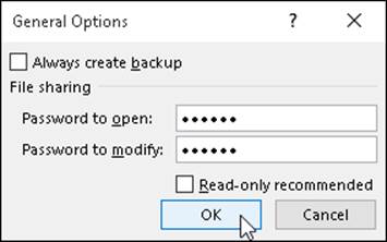
Figure 1-1: Setting a password to open and modify the workbook in the General Options dialog box.

Select the Read-Only Recommended check box in the General Options dialog box instead of assigning a password for editing the workbook in the Password to Modify text box when you never want the user to be able to make and save changes in the same workbook file. When Excel marks a file as read-only, the user must save any modifications in a different file using the Save As command. (See “Entering a password to make editing changes” later in this chapter for more on working with a read-only workbook file.)

Assigning a password to open from the Info screen

Instead of assigning the password to open your workbook at the time you save changes to it, you can do this as well from Excel 2016’s Info screen in the Backstage view by following these simple steps:

1. Choose File  ⇒  Info or press Alt+FI.

Excel opens the Info screen.

2. Click the Protect Workbook button to open its drop-down menu and then choose Encrypt with Password.

Excel opens the Encrypt Document dialog box.

3. Type the password exactly as you entered it in the Password text box and then select OK.

Excel opens the Confirm Password dialog box.

4. Type the password in the Reenter Password text box exactly as you typed it into the Password text box in the Encrypt Document dialog box and then select OK.

Note that if you don’t replicate the password exactly, Excel displays an alert dialog box indicating that the confirmation password is not identical. After you click OK to close this alert dialog box, you’re returned to the Confirm Password dialog box.

After successfully replicating the password, Excel closes the Confirm Password dialog box and returns you to the Info screen, where “A password is required to open this workbook” status message now appears under the Protect Workbook heading.

5. Click the Save option on the Info screen.

Excel closes the Backstage and returns you to the regular worksheet window as the program saves your new password to open as part of the workbook file.

Keep in mind that the drop-down menu attached to the Protect Workbook button in the Info screen in the Backstage does not contain an option for protecting the workbook from further modification after it’s opened in Excel. Instead, it contains a Mark as Final option that assigns read-only status to the workbook file that prevents the user from saving changes to the file under the same filename.

Entering the password to gain access

After you save a workbook file to which you’ve assigned a password for opening it, you must thereafter be able to faithfully reproduce the password in order to open the file (at least until you change or delete the password). When you next try to open the workbook, Excel opens a Password dialog box like the one shown in Figure 1-2, where you must enter the password exactly as it was assigned to the file.

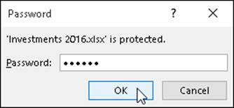
Figure 1-2: Entering the password required to open a protected workbook file.

If you mess up and type the wrong password, Excel displays an alert dialog box letting you know that the password you entered is incorrect. When you click OK to clear the alert, you are returned to the original Excel window where you must repeat the entire file-opening procedure (hoping that this time you’re able to enter the correct password). When you supply the correct password, Excel immediately opens the workbook for viewing and printing (and editing as well, unless you’ve also assigned a password for modifying the file). If you’re unable to successfully reproduce the password, you are unable to open the file and put it to any use!

The last chance you have to chicken out of password-protecting the opening of the file is before you close the file during the work session in which you originally assign the password. If, for whatever reason, you decide that you don’t want to go through the hassle of having to reproduce the password each and every time you open this file, you can get rid of it by choosing File  ⇒  Save As or pressing Alt+FA, choosing General Options from the Tools drop-down menu, and then deleting the password in the Password to Open text box before clicking OK in the General Options dialog box and the Save button in the Save As dialog box. Doing this resaves the workbook file without a password to open it so that you don’t have to worry about reproducing the password the next time you open the workbook for editing or printing.

A password-protected workbook file for which you can’t reproduce the correct password can be a real nightmare (especially if you’re talking about a really important spreadsheet with loads and loads of vital data). So, for heaven’s sake, don’t forget your password, or you’ll be stuck. Excel does not provide any sort of command for overriding the password and opening a protected workbook, nor does Microsoft offer any such utility. If you think that you might forget the workbook’s password, be sure to write it down somewhere and then keep that piece of paper in a secure place, preferably under lock and key. It’s always better to be safe than sorry when it comes to passwords for opening files.

Entering the password to make changes

If you’ve protected your workbook from modifications with the Password to Modify option in the General Options dialog box, as soon as you attempt to open the workbook (and have entered the password to open the file, if one has been assigned), Excel immediately displays the Password dialog box where you must accurately reproduce the password assigned for modifying the file or select the Read Only button to open it as a read-only file.

As when supplying the password to open a protected file, if you type the wrong password, Excel displays the alert dialog box letting you know that the password you entered is incorrect. When you click OK to clear the alert, you are returned to the Password dialog box, where you can try reentering the password in the Password text box.

When you supply the correct password, Excel immediately closes the Password dialog box, and you are free to edit the workbook in any way you wish (unless certain cell ranges or worksheets are protected). If you’re unable to successfully reproduce the password, you can click the Read Only command button, which opens a copy of the workbook file into which you can’t save your changes unless you use the File  ⇒  Save As command and then rename the workbook and/or locate the copy in a different folder.

When you click the Read Only button, Excel opens the file with a [Read-Only] indicator appended to the filename as it appears on the Excel title bar. If you then try to save changes with the Save button on the Quick Access toolbar or File  ⇒  Save command, the program displays an alert dialog box, indicating that the file is read-only and that you must save a copy by renaming the file in the Save As dialog box. As soon as you click OK to clear the alert dialog box, Excel displays the Save As dialog box, where you can save the copy under a new filename and/or location. Note that the program automatically removes the password for modifying from the copy so that you can modify its contents any way you like.

Because password-protecting a workbook against modification does not prevent you from opening the workbook and then saving an unprotected version under a new filename with the Save As command, you can assign passwords for modifying files without nearly as much trepidation as assigning them for opening files. Assigning a password for modifying the file assures you that you’ll always have an intact original of the spreadsheet from which you can open and save a copy, even if you can never remember the password to modify the original itself.

Changing or deleting a password

Before you can change or delete a password for opening a workbook, you must first be able to supply the current password you want to change to get the darned thing open. Assuming you can do this, all you have to do to change or get rid of the password is open the Info screen in the Backstage view (Alt+FI) and then choose the Encrypt with Password option from the Protect Workbook button’s drop-down menu.

Excel opens the Encrypt Document dialog box with your password in the Password text box masked by asterisks. To then delete the password, simply remove all the asterisks from this text box before you click OK.

To reassign the password, replace the current password with the new one you want to assign by typing it over the original one. Then, when you click OK in the Encrypt Document dialog box, reenter the new password in the Confirm Password dialog box and then click its OK button. Finally, after closing the Encrypt Document dialog box, you simply click the Save option on the File menu in the Backstage view to save your changes and return to the regular worksheet window.

To change or delete the password for modifying the workbook, you must do this from the General Options dialog box. Choose File  ⇒  Save As (Alt+FA) and then, after indicating the place to save the file in the Save As screen, choose the General Options item from the Tools drop-down menu in the Save As dialog box. You then follow the same procedure for changing or deleting the password that’s entered into the Password to Modify text box in the General Options dialog box.

Protecting the Worksheet

After you have the worksheet the way you want it, you often need the help of Excel’s Protection feature to keep it that way. Nothing’s worse than having an inexperienced data entry operator doing major damage to the formulas and functions that you’ve worked so hard to build and validate. To keep the formulas and standard text in a spreadsheet safe from any unwarranted changes, you need to protect the worksheet.

Before you start using the Protect Sheet and Protect Workbook command buttons on the Review tab of the Ribbon, you need to understand how protection works in Excel. All cells in the workbook are either locked or unlocked for editing and hidden or unhidden for viewing.

Whenever you begin a new spreadsheet, all the cells in the workbook have locked as their editing status and unhidden as their display status. However, this default editing and display status in and of itself does nothing until you turn on protection with the Protect Sheet and Protect Workbook command buttons on the Review tab. At that time, you are then prevented from making any editing changes to all cells with a locked status and from viewing the contents of all cells on the Formula bar when they contain the cell cursor with a hidden status.

What this means in practice is that, prior to turning on worksheet protection, you go through the spreadsheet removing the Locked Protection format from all the cell ranges where you or your users need to be able to do data entry and editing even when the worksheet is protected. You also assign the Hidden Protection format to all cell ranges in the spreadsheet where you don’t want the contents of the cell to be displayed when protection is turned on in the worksheet. Then, when that formatting is done, you activate protection for all the remaining Locked cells and block the Formula bar display for all the Hidden cells in the sheet.

When setting up your own spreadsheet templates, you will want to unlock all the cells where users need to input new data and keep locked all the cells that contain headings and formulas that never change. You may also want to hide cells with formulas if you’re concerned that their display might tempt the users to waste time trying to fiddle with or finesse them. Then, turn on worksheet protection prior to saving the file in the template file format. (See Book II, Chapter 1, for details.) You are then assured that all spreadsheets generated from that template automatically inherit the same level and type of protection as you assigned in the original spreadsheet.

Changing a cell’s Locked and Hidden Protection formatting

To change the status of cells from locked to unlocked or from unhidden to hidden, you use the Locked and Hidden check boxes found on the Protection tab of the Format Cells dialog box (Ctrl+1).

To remove the Locked protection status from a cell range or nonadjacent selection, you follow these two steps:

1. Select the range or ranges to be unlocked.

To select multiple ranges to create a nonadjacent cell selection, hold down the Ctrl key as you drag through each range.

2. Click the Format command button on the Ribbon’s Home tab and then choose the Lock option near the bottom of its drop-down menu or press Alt+HOL.

Excel lets you know that the cells that contain formulas in the selected range are no longer locked by adding tiny green triangles to the upper-left corner of each cell in the range that, when clicked, display an alert drop-down button whose tool tip reads, “This cell contains a formula and is not locked to protect it from being changed inadvertently.” When you click this alert button, a drop-down menu with Lock Cell as one of its menu items appears. Note that as soon as you turn on protection in the sheet, these indicators disappear.

You can also change the protection status of a selected range of cells with the Locked check box on the Protection tab of the Format Cells dialog box. Simply open the Format Cells dialog box (Ctrl+1), click the Protection tab, and then click the Locked check box to remove the check mark before you click OK.

To hide the display of the contents of the cells in the current selection, you click the Hidden check box instead of the Locked check box on the Protection tab of the Format Cells dialog box before you click OK.

Remember that changing the protection formatting of cell ranges in the worksheet (as described above) does nothing in and of itself. It’s not until you turn on the protection for your worksheet (as outlined in the next section) that your unlocked and hidden cells work or appear any differently from the locked and unhidden cells. At that time, only unlocked cells accept edits, and only unhidden cells display their contents on the Formula bar when they contain the cell cursor.

Protecting the worksheet

When you’ve gotten all cell ranges that you want unlocked and hidden correctly formatted in the worksheet, you’re ready to turn on protection. To do this, you click the Protect Sheet command button on the Ribbon’s Review tab or press Alt+RPS to open the Protect Sheet dialog box, shown in Figure 1-3.

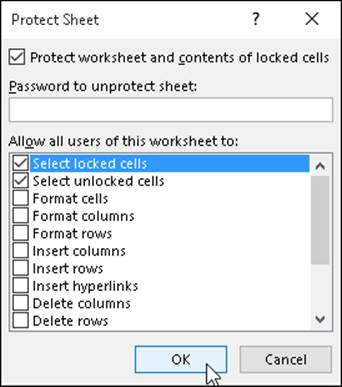
Figure 1-3: Selecting the protection options in the Protect Sheet dialog box.

When you first open this dialog box, only the Protect Worksheet and Contents of Locked Cells check box at the very top and the Select Locked Cells and Select Unlocked Cells check boxes in the Allow All Users of This Worksheet To list box are selected. All the other check box options (including some that are not visible without scrolling up the Allow All Users of This Worksheet To list box) are deselected.

This means that if you click OK at this point, the only things that you’ll be permitted to do in the worksheet are edit unlocked cells and select cell ranges (of any type: both locked and unlocked alike).

If you really want to keep other users out of all the locked cells in a worksheet, clear the Select Locked Cells check box in the Allow All Users of This Worksheet To list box to remove its check mark. That way, your users are completely restricted to just those unlocked ranges where you permit data input and content editing.

Don’t, however, deselect the Select Unlocked Cells check box as well as the Select Locked Cells check box, because doing this makes the cell pointer disappear from the worksheet, making the cell address in the Name Box on the Formula bar the sole way for you and your users to keep track of their position in the worksheet (which is, believe me, the quickest way to drive you and your users stark-raving mad).

Selecting what actions are allowed in a protected sheet

In addition to enabling users to select locked and unlocked cells in the worksheet, you can enable the following actions in the protected worksheet by selecting their check boxes in the Allow All Users of This Worksheet To list box of the Protect Sheet dialog box:

· Format Cells: Enables the formatting of cells (with the exception of changing the locked and hidden status on the Protection tab of the Format Cells dialog box).

· Format Columns: Enables formatting so that users can modify the column widths and hide and unhide columns.

· Format Rows: Enables formatting so that users can modify the row heights and hide and unhide rows.

· Insert Columns: Enables the insertion of new columns in the worksheet.

· Insert Rows: Enables the insertion of new rows in the worksheet.

· Insert Hyperlinks: Enables the insertion of new hyperlinks to other documents, both local and on the web. (See Book IV, Chapter 2, for details.)

· Delete Columns: Enables the deletion of columns in the worksheet.

· Delete Rows: Enables the deletion of rows in the worksheet.

· Sort: Enables the sorting of data in unlocked cells in the worksheet. (See Book VI, Chapter 1, for details.)

· Use AutoFilter: Enables the filtering of data in the worksheet. (See Book VI, Chapter 2, for more information.)

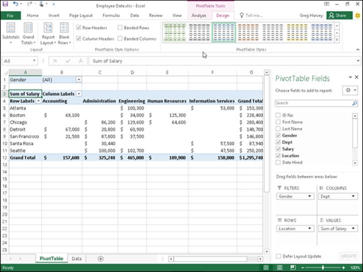
· Use PivotTable & PivotChart: Enables the manipulation of pivot tables and pivot charts in the worksheet. (For more about pivot tables, see Book VII, Chapter 2.)

· Edit Objects: Enables the editing of graphic objects, such as text boxes, embedded images, and the like, in the worksheet. (See Book V, Chapter 2, for details.)

· Edit Scenarios: Enables the editing of what-if scenarios, including modifying and deleting them. (For details of what-if scenarios, see Book VII, Chapter 1.)

Assigning a password to unprotect the sheet

In addition to enabling particular actions in the protected worksheet, you can also assign a password that’s required in order to remove the protections from the protected worksheet. When entering a password in the Password to Unprotect Sheet text box of the Protect Sheet dialog box, you observe the same guidelines as when assigning a password to open or to make changes in the workbook (255 characters maximum that can consist of a combination of letters, numbers, and spaces, with the letters being case-sensitive).

As with assigning a password to open or make changes to a workbook, when you enter a password (whose characters are masked with asterisks) in the Password to Unprotect Sheet text box and then click OK, Excel displays the Confirm Password dialog box. Here, you must accurately reproduce the password you just entered (including upper- and lowercase letters) before Excel turns on the sheet protection and assigns the password for removing protection.

If you don’t successfully reproduce the password, when you click OK in the Confirm Password dialog box, Excel replaces it with an alert dialog box indicating that the confirmation password is not identical to the one you entered in the Protect Sheet dialog box. When you click OK to clear this alert dialog box, you are returned to the Protect Sheet dialog box, where you may modify the password in the Password to Unprotect Sheet text box before you click OK and try confirming the password again.

As soon as you accurately reproduce the password in the Confirm Password dialog box, Excel closes the Protect Sheet dialog box and enables protection for that sheet, using whatever settings you designated in that dialog box.

If you don’t assign a password to unprotect the sheet, any user with a modicum of Excel knowledge can lift the worksheet protection and make any manner of changes to its contents, including wreaking havoc on its computational capabilities by corrupting its formulas. Keep in mind that it makes little sense to turn on the protection in a worksheet if you’re going to permit anybody to turn it off by simply clicking the Unprotect Sheet command button on the Review tab (which automatically replaces the Protect Sheet command button as soon as you turn on protection in the worksheet).

Removing protection from a worksheet

When you assign protection to a sheet, your input and editing are restricted solely to unlocked cells in the worksheet, and you can perform only those additional actions that you enabled in the Allow Users of this Worksheet To list box. If you try to replace, delete, or otherwise modify a locked cell in the protected worksheet, Excel displays an alert dialog box with the following message:

The cell or chart you’re trying to change is on a protected sheet.

The message then goes on to tell you

To make changes, click Unprotect Sheet in the Review tab (you might need a password).

If you’ve assigned a password to unprotect the sheet, when you click the Unprotect Sheet button, the program displays the Unprotect Sheet dialog box, where you must enter the password exactly as you assigned it. As soon as you remove the protection by entering the correct password in this dialog box and clicking OK, Excel turns off the protection in the sheet, and you can once again make any kinds of modifications to its structure and contents in both the locked and unlocked cells.

Keep in mind that when you protect a worksheet, only the data and graphics on that particular worksheet are protected. This means that you can modify the data and graphics on other sheets of the same workbook without removing protection. If you have data or graphics on other sheets of the same workbook that also need protecting, you need to activate that sheet and then repeat the entire procedure for protecting it as well (including unlocking cells that need to be edited and selecting which other actions, if any, to enable in the worksheet, and whether to assign a password to unprotect the sheet) before distributing the workbook. When assigning passwords to unprotect the various sheets of the workbook, you may want to stick with a single password rather than have to worry about remembering a different password for each sheet, which is a bit much, don’t you think?

Enabling cell range editing by certain users

You can use the Allow Users to Edit Ranges command button in the Changes group on the Review tab of the Ribbon to enable the editing of particular ranges in the protected worksheet by certain users. When you use this feature, you give certain users permission to edit particular cell ranges, provided that they can correctly provide the password you assign to that range.

To give access to particular ranges in a protected worksheet, you follow these steps:

1. Click the Allow Users to Edit Ranges command button on the Ribbon’s Review tab or press Alt+RU.

Note that the Allow Users to Edit Ranges command button is grayed out and unavailable if the worksheet is currently protected. In that case, you must remove protection by clicking the Unprotect Sheet command button on the Review tab before you retry Step 1.

Excel opens the Allow Users to Edit Ranges dialog box, where you can add the ranges you want to assign, as shown in Figure 1-4.

2. Click the New button.

Doing this opens the New Range dialog box where you give the range a title, define its cell selection, and provide the range password, as shown in Figure 1-5.

3. If you wish, type a name for the range in the Title text box; otherwise, Excel assigns a name such as Range1, Range2, and so on.

Next, you designate the cell range or nonadjacent cell selection to which access is restricted.

4. Click the Refers to Cells text box and then type in the address of the cell range (without removing the = sign) or select the range or ranges in the worksheet.

Next, you need to enter a password that’s required to get access to the range. Like all other passwords in Excel, this one can be up to 255 characters long, mixing letters, numbers, and spaces. Pay attention to the use of upper- and lowercase letters because the range password is case-sensitive.

5. Type in the password for accessing the range in the Range Password dialog box.

You need to use the Permissions button in the New Range dialog box to open the Permissions dialog box for the range you’re setting.

6. Click the Permissions button in the Range Password dialog box.

Next, you need to add the users who are to have access to this range.

7. Click the Add button in the Permissions dialog box.

Doing this opens the Select Users or Groups dialog box, where you designate the names of the users to have access to the range.

8. Click the name of the user in the Enter the Object Names to Select list box at the bottom of the Select Users or Groups dialog box. To select multiple users from this list, hold down the Ctrl key as you click each username.

If this list box is empty, click the Advanced button to expand the Select Users or Groups dialog box and then click the Find Now button to locate all users for your location. You can then click the name or Ctrl+click the names you want to add from this list, and then when you click OK, Excel returns you to the original form of the Select Users or Groups dialog box and adds these names to its Enter the Object Names to Select list box.

9. Click OK in the Select Users or Groups dialog box.

Doing this returns you to the Permissions dialog box where the names you’ve selected are now listed in the Group or User Names list box. Now you need to set the permissions for each user. When you first add users, each one is permitted to edit the range without a password. To restrict the editing to only those who have the range password, you need to click each name and then select the Deny check box.

10. Click the name of the first user who must know the password and then select the Deny check box in the Permissions For list box.

You need to repeat this step for each person in the Group or User Names list box that you want to restrict in this manner. (See Figure 1-6.)

11. Repeat Step 10 for each user who must know the password and then click OK in the Permissions dialog box.

As soon as you click OK, Excel displays a warning alert dialog box, letting you know that you are setting a deny permission that takes precedence over any allowed entries, so that if the person is a member of two groups, one with an Allow entry and the other with a Deny entry, the deny entry permission rules (meaning that the person has to know the range password).

12. Click the Yes button in the Security alert dialog box.

Doing this closes this dialog box and returns you to the New Range dialog box.

13. Click OK in the New Range dialog box.

Doing this opens the Confirm Password dialog box where you must accurately reproduce the range password.

14. Type the range password in the Reenter Password to Proceed text box and then click the OK button.

Doing this returns you to the Allow Users to Edit Ranges dialog box where the title and cell reference of the new range are displayed in the Ranges Unlocked by a Password When Sheet Is Protected list box, as shown in Figure 1-7.

If you need to define other ranges available to other users in the worksheet, you can do so by repeating Steps 2 through 14.

When you finish adding ranges to the Allow Users to Edit Ranges dialog box, you’re ready to protect the worksheet. If you want to retain a record of the ranges you’ve defined, go to Step 15. Otherwise, skip to Step 16.

15. (Optional) Select the Paste Permissions Information Into a New Workbook check box if you want to create a new workbook that contains all the permissions information.

When you select this check box, Excel creates a new workbook whose first worksheet lists all the ranges you’ve assigned, along with the users who may gain access by providing the range password. You can then save this workbook for your records. Note that the range password is not listed on this worksheet — if you want to add it, be sure that you password-protect the workbook so that only you can open it.

Now, you’re ready to protect the worksheet. If you want to do this from within the Allow Users to Edit Ranges dialog box, you click the Protect Sheet button to open the Protect Sheet dialog box. If you want to protect the worksheet later on, you click OK to close the Allow Users to Edit Ranges dialog box and then click the Protect Sheet command button on the Review tab of the Ribbon (or press Alt+RPS) when you’re ready to activate the worksheet protection.

16. Click the Protect Sheet button to protect the worksheet; otherwise, click the OK button to close the Allow Users to Edit Ranges dialog box.

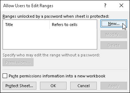
Figure 1-4: Designating the range to be unlocked by a password in a protected worksheet.

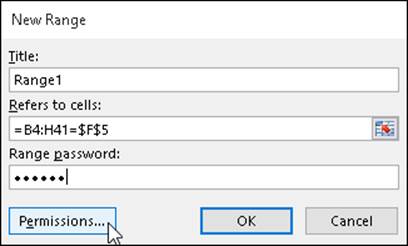
Figure 1-5: Assigning the range title, address, and password in the New Range dialog box.

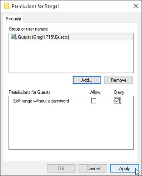
Figure 1-6: Setting the permissions for each user in the Permissions dialog box.

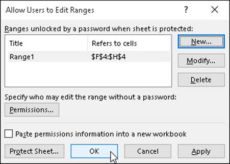
Figure 1-7: Getting ready to protect the sheet in the Allow Users to Edit Ranges dialog box.

If you click the Protect Sheet button, Excel opens the Protect Sheet dialog box, where you can set a password to unprotect the sheet. This dialog box is also where you select the actions that you permit all users to perform in the protected worksheet (as outlined earlier in this chapter).

After you turn on protection in the worksheet, only the users you’ve designated are able to edit the cell range or ranges you’ve defined. Of course, you need to supply the range password to all the users allowed to do editing in the range or ranges at the time you distribute the workbook to them.

Be sure to assign a password to unprotect the worksheet at the time you protect the worksheet if you want to prevent unauthorized users from being able to make changes to the designated editing ranges in the worksheet. If you don’t, any user can make changes by turning off the worksheet protection and thereby gaining access to the Allow Users to Edit Ranges command by clicking the Unprotect Sheet command button on the Review tab of the Ribbon.

Doing data entry in the unlocked cells of a protected worksheet

The best part of protecting a worksheet is that you and your users can jump right to unlocked cells and avoid even dealing with the locked ones (that you can’t change, anyway) by using the Tab and Shift+Tab keys to navigate the worksheet. When you press the Tab key in a protected worksheet, Excel jumps the cell cursor to the next unlocked cell to the right of the current one in that same row. When you reach the last unlocked cell in that row, the program then jumps to the first unlocked cell in the rows below. To move back to a previous unlocked cell, you press Shift+Tab. When Excel reaches the last unlocked cell in the spreadsheet, it automatically jumps back to the very first unlocked cell on the sheet.

Of course, provided that you haven’t changed the behavior of the Enter key in the Editing Options section on the Advanced tab of the Excel Options dialog box (File  ⇒  Options or Alt+FI), you can also use the Enter key to move down the columns instead of across the rows. However, pressing the Enter key to progress down a column selects locked cells in that column as well as the unlocked ones, whereas pressing the Tab key skips all those cells with the Locked protection format.

Figure 1-8 illustrates how you can put the Tab key to good use in filling out and navigating a protected worksheet. This figure shows a worksheet created from a Spa Holiday Hot Tubs invoice template. Because this invoice worksheet in the original template is protected, all worksheets generated from the template will be protected as well. The only cells that are unlocked in this sheet are the cells in the following ranges:

· F4:F6 with the invoice number, date, and customer ID fields

· C9:C13 with the name, company name, street address, city, state and zip, and phone number fields

· C16:D16 with the salesperson and job fields

· Cell G16 with the due date field

· C19:F38 with the quantity, description, and unit price fields

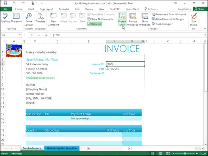
Figure 1-8: Using the Tab key to move from unlocked cell to unlocked cell in a protected worksheet.

All the rest of the cells in this worksheet are locked and off limits.

To fill in the data for this new invoice, you can press the Tab key to complete the data entry in each field such as Invoice No., Date, Customer ID, Name, Company Name, Street Address, and so on. By pressing Tab, you don’t have to waste time moving through the locked cells that contain headings that you can’t modify anyway. If you need to back up and return to the previous field in the invoice, you just press Shift+Tab to go back to the previous unlocked cell.

To make it impossible for the user to select anything but the unlocked cells in the protected worksheet, you clear the Select Locked Cells check box in the Allow All Users of This Worksheet To list box of the Protect Sheet dialog box.

Protecting the workbook

There is one last level of protection that you can apply to your spreadsheet files, and that is protecting the entire workbook. When you protect the workbook, you ensure that its users can’t change the structure of the file by adding, deleting, or even moving and renaming any of its worksheets. To protect your workbook, you click the Protect Workbook command button on the Ribbon’s Review tab and then select the Protect Structure and Windows option from its drop-down menu (or press Alt+RPW).

Excel displays a Protect Structure and Windows dialog box like the one shown in Figure 1-9. This dialog box contains two check boxes: Structure (which is automatically selected) and Windows (which is not selected). This dialog box also contains a Password (Optional) text box where you can enter a password that must be supplied before you can unprotect the workbook. Like every other password in Excel, the password to unprotect the workbook can be up to 255 characters maximum, consisting of a combination of letters, numbers, and spaces, with all the letters being case-sensitive.

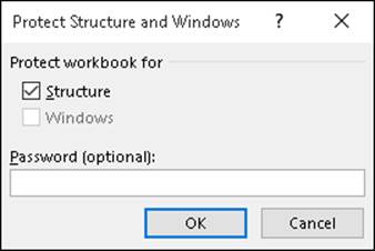
Figure 1-9: Protecting a workbook in the Protect Structure and Windows dialog box.

When you protect a workbook with the Structure check box selected, Excel prevents you or your users from doing any of the following tasks to the file:

· Inserting new worksheets

· Deleting existing worksheets

· Renaming worksheets

· Hiding or viewing hidden worksheets

· Moving or copying worksheets to another workbook

· Displaying the source data for a cell in a pivot table or displaying a table’s Report Filter fields on separate worksheets (see Book VII, Chapter 2, for details)

· Creating a summary report with the Scenario Manager (see Book VII, Chapter 1, for details)

When you turn on protection for a workbook after selecting the Windows check box in the Protect Structure and Windows dialog box, Excel prevents you from changing the size or position of the workbook’s windows (not usually something you need to control).

After you’ve enabled protection in a workbook, you can then turn it off by choosing the Protect Structure and Windows option on the Unprotect Workbook command button’s drop-down menu or by pressing Alt+RPW again. If you’ve assigned a password to unprotect the workbook, you must accurately reproduce it in the Password text box in the Unprotect Workbook dialog box that then appears.

Protecting a shared workbook

Many times you will want to protect a workbook that you intend to share on a network. That way, you can allow simultaneous editing of the contents of its worksheets (assuming that you don’t also protect individual sheets), while at the same time preventing anybody but you from removing the Change tracking (and thus deleting the Change History log — see Book IV, Chapter 3).

If the workbook is not currently shared, you can both protect the workbook and share it by clicking the Protect and Share Workbook command button on the Ribbon’s Review tab or by pressing Alt+RO. Note that if the workbook is already shared, you must stop sharing the file before you can use this command. (See Book IV, Chapter 4, for details on how to do this.)

When you click the Protect and Share Workbook command button, Excel opens the Protect Shared Workbook dialog box, similar to the one shown in Figure 1-10. In this dialog box, you select the Sharing with Track Changes check box to enable file sharing and to turn on the Change tracking. As soon as you select this check box, Excel makes available the Password (Optional) text box, where you can enter a password that must be supplied before you can stop sharing the workbook.

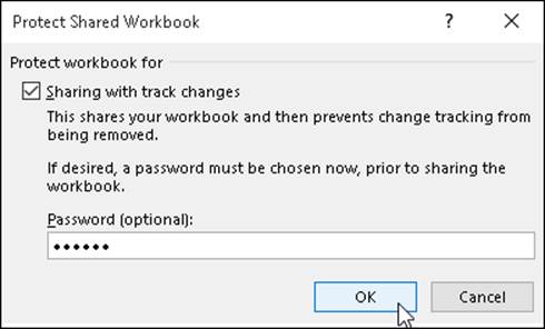
Figure 1-10: Setting up protection for a shared workbook in the Protect Shared Workbook dialog box.

If you enter a password in this text box (and you should — otherwise, there’s little reason to use this option, because anyone can remove the protection from the shared workbook and thus stop the file sharing), Excel immediately displays the Confirm Password dialog box, where you must accurately reproduce the password.

When you do this, Excel displays an alert dialog box that informs you that it will now save the workbook, and when you click the Yes button, the program saves the workbook as a shared file and protects it from being made exclusive without the password. The program also adds a [Shared] indicator to the filename at the top of the Excel program window to let you know that the workbook is being shared.

To remove the protection from the shared workbook and, at the same time, stop sharing it, you choose the Unprotect Shared Workbook command button (that replaces the Protect Sharing button) in the Changes group on the Review tab of the Ribbon. After you enter the password to unprotect the file in the Unprotect Sharing dialog box and click OK, Excel displays an alert dialog box, informing you that your action is about to remove the file from shared use and erase the Change History log file. If you click Yes, you prevent users who are currently editing the workbook from saving their changes. If you’re sure that no one else is using the workbook, you can continue and remove the file sharing by clicking the Yes button.