Excel 2016 All-in-One For Dummies (2016)
Book IV
Worksheet Collaboration and Review
Chapter 2
Using Hyperlinks
In This Chapter
![]() Linking your spreadsheet to other Excel workbooks, Office documents, and web pages
Linking your spreadsheet to other Excel workbooks, Office documents, and web pages
![]() Linking to e-mail addresses
Linking to e-mail addresses
![]() Following the links that you create in the worksheet
Following the links that you create in the worksheet
![]() Editing hyperlinks in a worksheet
Editing hyperlinks in a worksheet
![]() Creating formulas that use the HYPERLINK function
Creating formulas that use the HYPERLINK function
The subject of this chapter is linking your worksheet with other documents through the use of hyperlinks. Hyperlinks are the kinds of links used on the web to take you immediately from one web page to another or from one website to another. Such links can be attached to text (thus the term, hypertext) or to graphics such as buttons or pictures. The most important aspect of a hyperlink is that it immediately takes you to its destination whenever you click the text or button to which it is attached.
In an Excel worksheet, you can create hyperlinks that take you to a different part of the same worksheet, to another worksheet in the same workbook, to another workbook or other type of document on your hard drive, or to a web page on your company’s intranet or on the World Wide Web.
Hyperlinks 101
To add hyperlinks in an Excel worksheet, you must define two things:
· The object to which you want to anchor the link and then click to activate
· The destination to which the link takes you when activated
The objects to which you can attach hyperlinks include any text that you enter into a cell or any graphic object that you draw or import into the worksheet. (See Book V, Chapter 2, for details on adding graphics to your worksheet.) The destinations that you can specify for links can be a new cell or range, the same workbook file, or another file outside the workbook.
The destinations that you can specify for hyperlinks that take you to another place in the same workbook file include
· The cell reference of a cell on any of the worksheets in the workbook that you want to go to when you click the hyperlink.
· The range name of the group of cells that you want to select when you click the hyperlink. The range name must already exist at the time you create the link.
The destinations that you can specify for hyperlinks that take you outside the current workbook include
· The filename of an existing file that you want to open when you click the hyperlink. This file can be another workbook file or any other type of document that your computer can open.
· The URL address of a web page that you want to visit when you click the hyperlink. This page can be on your company’s intranet or on the World Wide Web and is opened in your web browser.
· A new document that you want to create in Excel or some other program on your computer when you click the hyperlink. You must specify the filename and file extension (which indicates what type of document to create and what program to launch).
· An e-mail address for a new message that you want to create in your e-mail program when you click the hyperlink. You must specify the recipient’s e-mail address and the subject of the new message when you create the link.
Adding hyperlinks
The steps for creating a new hyperlink in the worksheet are very straightforward. The only thing you need to do beforehand is to add the jump text in the cell where you want the link or to draw or import the graphic object to which the link is to be attached (as described in Book V,Chapter 2). Then, to add a hyperlink to the text in this cell or the graphic object, follow these steps:
1. Position the cell pointer in the cell containing the text or click the graphic object to which you want to anchor the hyperlink.
After you have selected the cell with the text or the graphic object, you’re ready to open the Insert Hyperlink dialog box.
2. Click the Hyperlink command button on the Ribbon’s Insert tab or press Alt+NI or Ctrl+K.
The Insert Hyperlink dialog box opens (similar to the one shown in Figure 2-1). If you selected a graphic object or a cell that contains some entry besides text before opening this dialog box, you notice that the Text to Display text box contains <<Selection in Document>> and that this box is grayed out (because there isn’t any text to edit when anchoring a link to a graphic). If you selected a cell with a text entry, that entry appears in the Text to Display text box. You can edit this text in this box; however, be aware that any change that you make to it here is reflected in the current cell when you close the Insert Hyperlink dialog box.
The ScreenTip button located to the immediate right of the Text to Display text box enables you to add text describing the function of the link when you position the mouse pointer over the cell or graphic object to which the link is attached. To add a ScreenTip for your link, follow Step 3. Note that if you don’t add your own ScreenTip, Excel automatically creates its own ScreenTip that lists the destination of the new link when you position the mouse pointer on its anchor.
3. (Optional) Click the ScreenTip button and then type the text that you want to appear next to the mouse pointer in the Set Hyperlink ScreenTip dialog box before you click OK.
By default, Excel selects the Existing File or Web Page button in the Link To area on the left side of the Insert Hyperlink dialog box, thus enabling you to assign the link destination to a file on your hard drive or to a web page. To link to a cell or cell range in the current workbook, click the Place in This Document button. To link to a new document, click the Create New Document button. To link to a new e-mail message, click the E-Mail Address button.
4. Select the type of destination for the new link by clicking its button in the Link To panel on the left side of the Insert Hyperlink dialog box.
Now all that you need to do is to specify the destination for your link. How you do this depends on which type of link you’re adding; see the following instructions for details.
· Linking to a cell or named range in the current workbook: After clicking the Place in This Document button in the Link To panel, enter the address of the cell to link to in the Type the Cell Reference text box and then click the name of the sheet that contains this cell listed under the Cell Reference range in the Or Select a Place in This Document list box. To link to a named range, simply click its name under Defined Names in the Or Select a Place in This Document list box.
· Linking to an existing file: After clicking the Existing File or Web Page button in the Link To panel, open its folder in the Look In drop-down list box and then click its file icon in the list box that appears immediately below this box. If you’re linking to a web page, click the Address text box and enter the URL address (as in http:// and so on) there. If the file or web page that you select contains bookmarks (or range names, in the case of another Excel workbook) that name specific locations in the file to which you link, click the Bookmark button and then click the name of the location (bookmark) in the Select Place in Document dialog box before you click OK.
· Creating a new document: After clicking the Create New Document button in the Link To panel, enter a filename for the new document in the Name of New Document text box. Include the three-letter filename extension if this new document is not an Excel workbook, such as .doc to create a new Word document or .txt to create a new text file. To specify a different folder in which to create the new document, click the Change button to the right of the current path and then select the appropriate drive and folder in the Create New Document dialog box and click OK. If you want to edit the contents of the new document right away, leave the Edit the New Document Now option button selected. If you prefer to edit the new document at a later time, click the Edit the New Document Later option button.
· Creating a new e-mail message: After clicking the E-Mail Address button in the Link To panel, enter the e-mail address (as in gharvey@mindovermedia.com) in the E-Mail Address text box and then click the Subject text box and enter the subject of the new e-mail message.
5. Specify the destination for the new hyperlink by using the text boxes and list boxes that appear for the type of link destination that you selected.
Now you’re ready to create the link.
6. Click the OK button in the Insert Hyperlink dialog box.
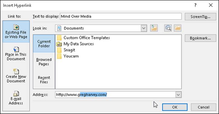
Figure 2-1: Creating a new hyperlink in the Insert Hyperlink dialog box.
As soon as you click OK, Excel closes the Insert Hyperlink dialog box and returns you to the worksheet with the new link (unless you specified that the new link is to create a new document and you left the Edit New Document Now option button selected, in which case, you’re in a new document — possibly in another application program such as Microsoft Word). If you anchored your new hyperlink to a graphic object, that object is still selected in the worksheet. (To deselect the object, click a cell outside its boundaries.) If you anchored your hyperlink to text in the current cell, the text now appears in blue and is underlined. (You may not be able to see the underlining until you move the cell cursor out of the cell.)
When you position the mouse pointer over the cell with the hypertext or the graphic object with the hyperlink, the mouse or Touch pointer changes from a thick, white cross to a hand with the index finger pointing upward. The ScreenTip that you assigned appears below and to the right of the hand mouse pointer.
If you didn’t assign your own ScreenTip to the hyperlink when creating it, Excel adds its own message that shows the URL destination of the link. If the link is a hypertext link (that is, if it’s anchored to a cell containing a text entry), the message in the ScreenTip also adds the following message:
Click once to follow. Click and hold to select this cell.
Follow that link!
To follow a hyperlink (assuming that your tablet or computer can connect to the Internet), click the link text or graphic object with the hand mouse or Touch pointer. Excel then takes you to the destination. If the destination is a cell in the workbook, Excel makes that cell current. If the destination is a cell range, Excel selects the range and makes the first cell of the range current. If this destination is a document created with another application program, Excel launches the application program (assuming that it’s available on the current computer). If this destination is a web page on the World Wide Web, Excel launches your web browser, connects you to the Internet, and then opens the page in the browser.
After you follow a hypertext link to its destination, the color of its text changes from the traditional blue to a dark shade of purple (without affecting its underlining). This color change indicates that the hyperlink has been followed. (Note, however, that graphic hyperlinks don’t show any change in color after you follow them.) Followed hypertext links regain their original blue color when you reopen their workbooks in Excel.
Editing hyperlinks
 Excel makes it easy to edit any hyperlink that you’ve added to your spreadsheet. The only trick to editing a link is that you have to be careful not to activate the link during the editing process. This means that you must always remember to right-click the link’s hypertext or graphic to select the link that you want to edit because clicking results only in activating the link.
When you right-click a link, Excel displays its shortcut menu. If you want to modify the link’s destination or ScreenTip, click Edit Hyperlink on this shortcut menu. This action opens the Edit Hyperlink dialog box with the same options as the Insert Hyperlink dialog box (shown previously in Figure 2-1). You can then use the Link To buttons on the left side of the dialog box to modify the link’s destination or the ScreenTip button to add or change the ScreenTip text.
Removing a hyperlink
If you want to remove the hyperlink from a cell entry or graphic object without getting rid of the text entry or the graphic, right-click the cell or graphic and then click the Remove Hyperlink item on the cell’s or object’s shortcut menu.
If you want to clear the cell of both its link and text entry, click the Delete item on the cell’s shortcut menu. To get rid of a graphic object along with its hyperlink, right-click the object (this action opens its shortcut menu) and then immediately click the object to remove the shortcut menu without either deselecting the graphic or activating the hyperlink. At this point, you can press the Delete key to delete both the graphic and the associated link.
Copying and moving a hyperlink
When you need to copy or move a hyperlink to a new place in the worksheet, you can use either the drag-and-drop or the cut-and-paste method. Again, the main challenge to using either method is selecting the link without activating it because clicking the cell or graphic object containing the link results in catapulting you over to the link’s destination point.
To select a cell that contains hypertext, use the arrow keys to position the cell cursor in that cell or use the Go To feature (F5 or Ctrl+G) and enter the cell’s address in the Go To dialog box to move the cell cursor there. To select a graphic object that contains a hyperlink, right-click the graphic to select it as well as to display its shortcut menu, and then immediately click the graphic (with the left mouse button) to remove the shortcut menu while keeping the object selected.
After you have selected the cell or graphic with the hyperlink, you can move the link by clicking the Cut command button on the Home tab of the Ribbon (Ctrl+X) or copy it by clicking the Copy command button (Ctrl+C) and then paste it into its new position by clicking the Paste command button (Ctrl+V). When moving or copying hypertext from one cell to another, you can just click the cell where the link is to be moved or copied and then press the Enter key.
To move the selected link by using the drag-and-drop method, drag the cell or object with the mouse pointer (in the shape of a white arrowhead pointing to a black double-cross) and then release the mouse button to drop the hypertext or graphic into its new position. To copy the link, be sure to hold down the Ctrl key (which changes the pointer to a white arrowhead with a plus sign to its right) as you drag the outline of the cell or object.
When attempting to move or copy a cell by using the drag-and-drop method, remember that you have to position the thick, white-cross mouse pointer on one of the borders of the cell before the pointer changes to a white arrowhead pointing to a black double-cross. If you position the pointer anywhere within the cell’s borders, the mouse changes to the hand with the index finger pointing upward, indicating that the hyperlink is active.
Using the HYPERLINK Function
Instead of using the Hyperlink command button on the Insert tab of the Ribbon, you can use Excel’s HYPERLINK function to create a hypertext link. (You can’t use this function to attach a hyperlink to a graphic object.) The HYPERLINK function uses the following syntax:
HYPERLINK(link_location,[friendly_name])
The link_location argument specifies the name of the document to open on your local hard drive, on a network server (designated by a UNC address), or on the company’s intranet or the World Wide Web (designated by the URL address — see the sidebar, “How to tell a UNC from a URL address and when to care,” for details). The optional friendly_name argument is the hyperlink text that appears in the cell where you enter the HYPERLINK function. If you omit this argument, Excel displays the text specified as the link_location argument in the cell.
How to tell a UNC from a URL address and when to care
The address that you use to specify a remote hyperlink destination comes in two basic flavors: UNC (Universal Naming Convention) and the more familiar URL (Universal Resource Locator). The type of address that you use depends on whether the destination file resides on a server on a network (in which case, you use a UNC address) or on a corporate intranet or the Internet (in which case, you use a URL address). Note that URLs also appear in many flavors, the most popular being those that use the Hypertext Transfer Protocol (HTTP) and begin with http:// and those that use the File Transfer Protocol (FTP) and start with ftp://.
The UNC address for destination files on network servers start with two backslash characters (\\), following this format:
\\server\share\path\filename
In this format, the name of the file server containing the file replaces server, the name of the shared folder replaces share, the directory path specifying any subfolders of the shared folder replaces path, and the file’s complete filename (including any filename extension, such as .xls for Excel worksheet) replaces filename.
The URL address for files published on websites follows this format:
internet service//internet address/path/filename
In this format, internet service is replaced with the Internet protocol to be used (either HTTP or FTP in most cases), internet address is replaced with the domain name (such as www.dummies.com) or the number assigned to the internet server, path is the directory path of the file, and filename is the complete name (including filename extensions such as .htm or .html for web pages).
When specifying the arguments for a HYPERLINK function that you type on the Formula bar (as opposed to one that you create by using the Insert Function feature by filling in the text boxes in the Function Arguments dialog box), you must remember to enclose both the link_locationand friendly_name arguments in closed double quotes. For example, to enter a HYPERLINK function in a cell that takes you to the home page of the For Dummies website and displays the text “Dummies Home Page” in the cell, enter the following in the cell:
=HYPERLINK("http://www.dummies.com","Dummies Home Page")