Excel 2016 All-in-One For Dummies (2016)

Book II

Worksheet Design

Chapter 2

Formatting Worksheets

In This Chapter

Selecting cell ranges and adjusting column widths and row heights

Formatting cell ranges as tables

Assigning number formats

Making alignment, font, border, and pattern changes

Using the Format Painter to quickly copy formatting

Formatting cell ranges with Cell Styles

Applying conditional formatting

Formatting — the subject of this chapter — is the process by which you determine the final appearance of the worksheet and the data that it contains. Excel’s formatting features give you a great deal of control over the way the data appears in your worksheet.

For all types of cell entries, you can assign a new font, font size, font style (such as bold, italics, underlining, or strikethrough), or color. You can also change the alignment of entries in the cells in a variety of ways, including the horizontal alignment, the vertical alignment, or the orientation; you can also wrap text entries in the cell or center them across the selection. For numerical values, dates, and times, you can assign one of the many built-in number formats or apply a custom format that you design. For the cells that hold your entries, you can apply different kinds of borders, patterns, and colors. And to the worksheet grid itself, you can assign the most suitable column widths and row heights so that the data in the formatted worksheet is displayed at its best.

With the FORMATTING and TABLES options on the Quick Analysis tool and the readily available mini-bar with its commonly used formatting buttons, formatting selected data tables in an Excel worksheet has never been easier or quicker. If those features are not enough, you still have access to the Table Styles and Cell Styles galleries and all the command buttons in the Font, Alignment, and Number groups on the Home tab of the Ribbon to get your spreadsheet data looking just right.

This is because Excel’s Live Preview feature enables you to see how a new font, font size, or table or cell style would look on your selected data before you actually apply it (saving you tons of time otherwise wasted applying format after format until you finally select the right one). And thanks to having buttons for all the most commonly used formatting commands right up front on the Home tab, you can now readily fine-tune the formatting of a cell in a worksheet by making almost all needed changes right from the Ribbon.

A range by any other name

Cell ranges are always noted in formulas by the first and last cell that you select, separated by a colon (:); therefore, if you select cell A1 as the first cell and cell H10 as the last cell and then use the range in a formula, the cell range appears as A1:H10. This same block of cells can just as well be noted as H10:A1 if you selected cell H10 before cell A1. Likewise, the same range can be equally noted as H1:A10 or A10:H1, depending upon which corner cell you select first and which opposite corner you select last. Keep in mind that despite the various range notations that you can use (A1:H10, H10:A1, H1:A10, and A10:H1), you are working with the same block of cells, the main difference being that each has a different active cell whose address appears in the Name box on the Formula bar (A1, H10, H1, and A10, respectively).

Making Cell Selections

Although you have to select the cells of the worksheet that you want to work with before you can accomplish many tasks used in building and editing a typical spreadsheet, perhaps no task requires cell selection like that of formatting. With the exception of the special Format as Table feature (which automatically selects the table to which its multiple formats are applied), selecting the cells whose appearance you want to enhance or modify is always your first step in their formatting.

In Excel, you can select a single cell, a block of cells (known as a cell range), or various discontinuous cell ranges (also known as a nonadjacent selection). Figure 2-1 shows a nonadjacent selection that consists of several different cell ranges (the smallest range is the single cell I9).

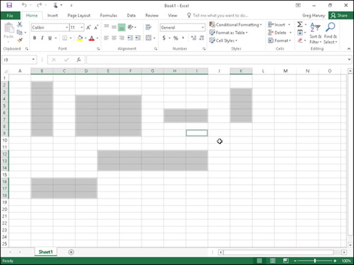
Figure 2-1: Worksheet with a nonadjacent cell selection made up of several different sized ranges.

Note that a simple cell selection consisting of a single cell range is denoted in the worksheet both by highlighting the selected cells in a light blue color as well as by extending the border of the cell cursor so that it encompasses all the highlighted cells. In a nonadjacent cell selection, however, all selected cells are highlighted but only the active cell (the one whose address is displayed in the Name Box on the Formula bar) contains the cell cursor (whose borders are quite thin when compared to the regular cell cursor).

Selecting cells with the mouse

Excel offers several methods for selecting cells with the mouse. With each method, you start by selecting one of the cells that occupies the corner of the range that you want to select. The first corner cell that you click becomes the active cell (indicated by its cell reference in the Formula bar), and the cell range that you then select becomes anchored on this cell.

After you select the active cell in the range, drag the pointer to extend the selection until you have highlighted all the cells that you want to include. Here are some tips:

· To extend a range in a block that spans several columns, drag left or right from the active cell.

· To extend a range in a block that spans several rows, drag up or down from the active cell.

· To extend a range in a block that spans several columns and rows, drag diagonally from the active cell in the most logical directions (up and to the right, down and to the right, up and to the left, or down and to the left).

If you ever extend the range too far in one direction, you can always reduce it by dragging in the other direction. If you’ve already released the mouse button and you find that the range is incorrect, click the active cell again. (Clicking any cell in the worksheet deselects a selected range and activates the cell that you click.) Then select the range of cells again.

You can always tell which cell is the active cell forming the anchor point of a cell range because it is the only cell within the range that you’ve selected that isn’t highlighted and is the only cell reference listed in the Name box on the Formula bar. As you extend the range by dragging the thick white-cross mouse pointer, Excel indicates the current size of the range in columns and rows in the Name box (as in 5R x 2C when you’ve highlighted a range of five rows long and two columns wide). However, as soon as you release the mouse button, Excel replaces this row and column notation with the address of the active cell.

You can also use the following shortcuts when selecting cells with the mouse:

· To select a single-cell range, click the thick white-cross mouse pointer somewhere inside the cell.

· To select all cells in an entire column, position the mouse pointer on the column letter in the column header and then click the mouse button. To select several adjacent columns, drag through their column letters in the column header.

· To select all cells in an entire row, position the mouse pointer on the row number in the row header and then click the mouse button. To select several adjacent rows, drag through the row numbers in the row header.

· To select all the cells in the worksheet, click the box in the upper-left corner of the worksheet at the intersection of row and column headers with the triangle in the lower-right corner that makes it look like the corner of a dog-eared or folded down book page. (You can also do this from the keyboard by pressing Ctrl+A.)

· To select a cell range composed of partial columns and rows without dragging, click the cell where you want to anchor the range, hold down the Shift key, and then click the last cell in the range and release the Shift key. (Excel selects all the cells in between the first and the last cell that you click.) If the range that you want to mark is a block that spans several columns and rows, the last cell is the one diagonally opposite the active cell. When using this Shift+click technique to mark a range that extends beyond the screen, use the scroll bars to display the last cell in the range. (Just make sure that you don’t release the Shift key until after you’ve clicked this last cell.)

· To select a nonadjacent selection comprised of several discontinuous cell ranges, drag through the first cell range and then hold down the Ctrl key as you drag through the other ranges. After you have marked all the cell ranges to be included in the nonadjacent selection, you can release the Ctrl key.

Selecting cells by touch

If you’re running Excel 2016 on a touchscreen device such as a Windows tablet or smartphone without the benefit of a mouse or physical keyboard, you can use your finger or stylus to make your cell selections:

· To use your finger, tap the first cell in the selection (the equivalent of clicking with a mouse). Selection handles (with the circle icons) appear in the upper-left and lower-right corner of the selected cell. Simply drag or swipe one of the selection handles through the rest of the adjacent cells to extend the cell selection and select the entire range.

· To use your tablet’s stylus, tap the first cell and then drag the white-cross pointer to the last cell in the selection.

Selecting cells with the keyboard

Excel also makes it easy for you to select cell ranges with a physical or Touch keyboard by using a technique known as extending a selection. To use this technique, you move the cell cursor to the active cell of the range; then press F8 to turn on Extend Selection mode (indicated by Extend Selection on the Status bar) and use the direction keys to move the pointer to the last cell in the range. Excel selects all the cells that the cell cursor moves through until you turn off Extend Selection mode (by pressing F8 again).

You can use the mouse as well as the keyboard to extend a selection when Excel is in Extend Selection mode. All you do is click the active cell, press F8, and then click the last cell to mark the range.

You can also select a cell range with the keyboard without turning on Extend Selection mode. Here, you use a variation of the Shift+click method by moving the cell pointer to the active cell in the range, holding down the Shift key, and then using the direction keys to extend the range. After you’ve highlighted all the cells that you want to include, release the Shift key.

To mark a nonadjacent selection of cells with the keyboard, you need to combine the use of Extend Selection mode with that of Add to Selection mode. To turn on Add to Selection mode (indicated by Add to Selection on the status bar), you press Shift+F8. To mark a nonadjacent selection by using Extend Selection and Add to Selection modes, follow these steps:

1. Move the cell cursor to the first cell of the first range you want to select.

2. Press F8 to turn on Extend Selection mode.

3. Use the arrow keys to extend the cell range until you’ve highlighted all its cells.

4. Press Shift+F8 to turn off Extend Selection mode and turn on Add to Selection mode instead.

5. Move the cell cursor to the first cell of the next cell range you want to add to the selection.

6. Press F8 to turn off Add to Selection mode and turn Extend Selection mode back on.

7. Use the arrow keys to extend the range until all cells are highlighted.

8. Repeat Steps 4 through 7 until you’ve selected all the ranges that you want included in the nonadjacent selection.

9. Press F8 to turn off Extend Selection mode.

You AutoSelect that range!

Excel’s AutoSelect feature provides a particularly efficient way to select all or part of the cells in a large table of data. AutoSelect automatically extends a selection in a single direction from the active cell to the first nonblank cell that Excel encounters in that direction.

You can use the AutoSelect feature with the mouse and a physical keyboard. The general steps for using AutoSelect to select a table of data with the mouse are as follows:

1. Click the first cell to which you want to anchor the range that you are about to select.

In a typical data table, this cell may be the blank cell at the intersection of the row of column headings and the column of row headings.

2. Position the mouse pointer on the edge of the cell in the direction you want to extend the range.

To extend the range up to the first blank cell to the right, position the mouse or Touch pointer on the right edge of the cell. To extend the range left to the first blank cell, position the pointer on the left edge of the cell. To extend the range down to the first blank cell, position the pointer on the bottom edge of the cell. And to extend the range up to the first blank cell, position the pointer on the top edge of the cell.

3. When the pointer changes shape from a cross to an arrowhead, hold down the Shift key and then double-click the mouse.

As soon as you double-click the mouse or Touch pointer, Excel extends the selection to the first occupied cell that is adjacent to a blank cell in the direction of the edge that you double-clicked.

To get an idea of how AutoSelect works, consider how you use it to select all the data in the table (cell range A3:J8) shown in Figures 2-2 and 2-3. With the cell cursor in cell A3 at the intersection of the row with the Date column headings and the column with the Part row headings, you can use the AutoSelect feature to select all the cells in the table in two operations:

· In the first operation, hold down the Shift key and then double-click the bottom edge of cell A2 to highlight the cells down to A6, selecting the range A2:A6. (See Figure 2-2.)

· In the second operation, hold down the Shift key and then double-click the right edge of cell range A2:A6 to extend the selection to the last column in the table (selecting the entire table with the cell range A2:J6, as shown in Figure 2-3).

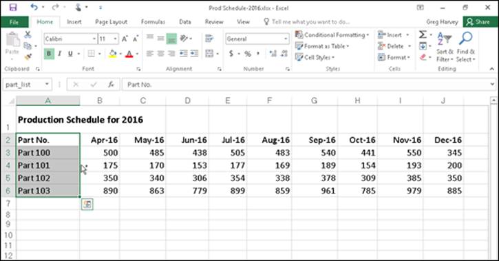
Figure 2-2: Selecting the cells in the first column of the table with AutoSelect.

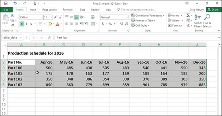
Figure 2-3: Selecting all the remaining columns of the table with AutoSelect.

If you select the cells in the first row of the table (range A2:J2) in the first operation, you can then extend this range down the remaining rows of the table by double-clicking the bottom edge of one of the selected cells. (It doesn’t matter which one.)

To use the AutoSelect feature with the keyboard, press the End key and one of the four arrow keys as you hold down the Shift key. When you hold down Shift and press End and an arrow key, Excel extends the selection in the direction of the arrow key to the first cell containing a value that is bordered by a blank cell.

In terms of selecting the table of data shown in Figures 2-2 and 2-3, this means that you would have to complete four separate operations to select all of its cells:

1. With A2 as the active cell, hold down Shift and press End+↓ to select the range A2:A6.

Excel stops at A6 because this is the last occupied cell in that column. At this point, the cell range A2:A6 is selected.

2. Hold down Shift and then press End+→.

Excel extends the range all the way to column J (because the cells in column J contain entries bordered by blank cells). Now all the cells in the table (the cell range A2:J6) are selected.

Selecting cells with Go To

Although you usually use the Go To feature to move the cell cursor to a new cell in the worksheet, you can also use this feature to select a range of cells. When you choose the Go To option from the Find & Select button’s drop-down menu on the Home tab of the Ribbon (or press Ctrl+G or F5), Excel displays a Go To dialog box similar to the one shown in Figure 2-4. To move the cell cursor to a particular cell, enter the cell address in the Reference text box and click OK. (Excel automatically lists the addresses of the last four cells or cell ranges that you specified in the Go To list box.)

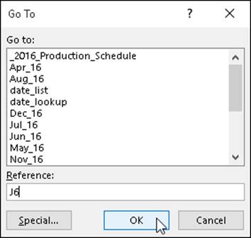
Figure 2-4: Selecting a cell range with the Go To dialog box.

Instead of just moving to a new section of the worksheet with the Go To feature, you can select a range of cells by taking these steps:

1. Select the first cell of the range.

This becomes the active cell to which the cell range is anchored.

2. On the Ribbon, click the Find & Select command button in the Editing group on the Home tab and then choose Go To from its drop-down menu or press Alt+HFDG, Ctrl+G or F5.

The Go To dialog box opens.

3. Type the cell address of the last cell in the range in the Reference text box.

If this address is already listed in the Go To list box, you can enter this address in the text box by clicking it in the list box.

4. Hold down the Shift key as you click OK or press Enter to close the Go To dialog box.

By holding down Shift as you click OK or press Enter, you select the range between the active cell and the cell whose address you specified in the Reference text box.

Instead of selecting the anchor cell and then specifying the last cell of a range in the Reference text box of the Go To dialog box, you can also select a range simply by typing in the address of the cell range in the Reference text box. Remember that when you type a range address, you enter the cell reference of the first (active) cell and the last cell in the range separated by a colon. For example, to select the cell range that extends from cell B2 to G10 in the worksheet, you would type the range address B2:G10 in the Reference text box before clicking OK or pressing Enter.

Name that range!

One of the easiest ways to select a range of data is to assign a name to it and then choose that name on the pop-up menu attached to the Name box on the Formula bar or in the Go To list box in the Go To dialog box. Of course, you reserve this technique for cell ranges that you work with on a somewhat regular basis; for example, ranges with data that you print regularly, consult often, or have to refer to in formula calculations. It’s probably not worth your while to name a range of data that doesn’t carry any special importance in the spreadsheet.

To name a cell range, follow three simple steps:

1. Select all the cells in the range that you intend to name.

You can use any of the cell selection techniques that you prefer. When selecting the cells for the named range, be sure to include all the cells that you want selected each time you select its range name.

2. Click the Name box on the Formula bar.

Excel automatically highlights the address of the active cell in the selected range.

3. Type the range name in the Name box and then press Enter.

As soon as you start typing, Excel replaces the address of the active cell with the range name that you’re assigning. As soon as you press the Enter key, the name appears in the Name box instead of the cell address of the active cell in the range.

When naming a cell range, however, you must observe the following naming conventions:

· Begin the range name with a letter of the alphabet rather than a number or punctuation mark.

· Don’t use spaces in the range name; instead, use an underscore between words in a range name (as in Qtr_1).

· Make sure that the range name doesn’t duplicate any cell reference in the worksheet by using either the standard A1 or R1C1 notation system.

· Make sure that the range name is unique in the worksheet.

After you’ve assigned a name to a cell range, you can select all its cells simply by clicking the name on the pop-up menu attached to the Name box on the Formula bar. The beauty of this method is that you can use it from anywhere in the same sheet or a different worksheet in the workbook because as soon as you click its name on the Name box pop-up menu, Excel takes you directly to the range, while at the same time automatically selecting all its cells.

Range names are also very useful when building formulas in your spreadsheet. For more on creating and using range names, see Book III, Chapter 1.

If you’re using a touchscreen device without access to a mouse or physical keyboard, I can’t recommend highly enough naming cell ranges that you regularly select for editing or printing in Excel 2016. Tapping the range name on the Name box’s drop-down menu to select a large and distant cell range in a worksheet on the normally very small and cramped screen of a Windows tablet is so far superior to futzing with the cell’s selection handles to select the range that it’s just not funny!

Adjusting Columns and Rows

Along with knowing how to select cells for formatting, you really also have to know how to adjust the width of your columns and the heights of your rows. Why? Because often in the course of assigning different formatting to certain cell ranges (such as new font and font size in boldface type), you may find that data entries that previously fit within the original widths of their column no longer do and that the rows that they occupy seem to have changed height all on their own.

In a blank worksheet, all the columns and rows are the same standard width and height. The actual number of characters or pixels depends upon the aspect ratio of the device upon which you’re running Excel 2016. On most computer monitors, all Excel 2016 worksheet columns start out 8.43 characters wide (or 64 pixels) and all rows start out 15 points high (or 20 pixels). On a smaller touchscreen such as the Microsoft Surface 3 tablet, Excel worksheet columns start out at 8.09 characters wide (or 96 pixels, given their distinctive aspect ratio) with rows at 13.50 characters or 27 pixels high.

As you build your spreadsheet, you end up with all sorts of data entries that can’t fit within these default settings. This is especially true as you start adding formatting to their cells to enhance and clarify their contents.

Most of the time, you don’t need to be concerned with the heights of the rows in your worksheet because Excel automatically adjusts them up or down to accommodate the largest font size used in a cell in the row and the number of text lines (in some cells, you may wrap their text on several lines). Instead, you’ll spend a lot more time adjusting the column widths to suit the entries for the formatting that you assign to them.

Remember what happens when you put a text entry in a cell whose current width isn’t long enough to accommodate all its characters. If the cells in columns to the right are empty, Excel lets the display of the extra characters spill over into the empty cells. If these cells are already occupied, however, Excel cuts off the display of the extra characters until you widen the column sufficiently. Likewise, remember that if you add formatting to a number so that its value and formatting can’t both be displayed in the cell, those nasty overflow indicators appear in the cell as a string of pound signs (#####) until you widen the column adequately.

You AutoFit the column to its contents

The easiest way to adjust the width of a column to suit its longest entry is to use the AutoFit feature. AutoFit determines the best fit for the column or columns selected at that time, given their longest entries.

· To use AutoFit on a single column: Position the mouse pointer on the right edge of that column in the column header and then, when the pointer changes to a double-headed arrow, double-click the mouse or double-tap your finger or stylus.

· To use AutoFit on multiple columns at one time: Select the columns by dragging through them in the column header or by Ctrl+clicking the column letters, and then double-clicking the right edge of one of the selected columns when the pointer changes to a double-headed arrow.

These AutoFit techniques work well for adjusting all columns except for those that contain really long headings (such as the spreadsheet title that often spills over several blank columns in row 1), in which case AutoFit makes the columns far too wide for the bulk of the cell entries.

For those situations, use the AutoFit Selection command, which adjusts the column width to suit only the entries in the cells of the column that you have selected. This way, you can select all the cells except for any really long ones in the column that purposely spill over to empty cells on the right, and then have Excel adjust the width to suit. After you’ve selected the cells in the column that you want the new width to fit, click the Format button in the Cells group on the Home tab and then choose AutoFit Selection from the drop-down menu.

Adjusting columns the old fashioned way

AutoFit is nothing if not quick and easy. If you need more precision in adjusting your column widths, you have to do this manually either by dragging its border with the mouse or by entering new values in the Column Width dialog box.

· To manually adjust a column width with the mouse: Drag the right edge of that column onto the Column header to the left (to narrow) or to the right (to widen) as required. As you drag the column border, a ScreenTip appears above the mouse pointer indicating the current width in both characters and pixels. When you have the column adjusted to the desired width, release the mouse button to set it.

· To manually adjust a column width by touch: Tap the right edge of the column header with your finger or stylus to select the column and make the black, double-header pointer appear. Then swipe the pointer left or right as needed. As you swipe, the Name box on the Formula bar indicates the current width in characters and pixels. When you have the column adjusted to the desired width, remove your finger or stylus from the touchscreen.

To make this operation easier, remember that you can instantly zoom in on the column border by stretching your forefinger and thumb on the touchscreen — doing this makes the column letter area larger, making it a lot easier to tap and swipe the border left and right with your finger or stylus.

· To adjust a column width in the Column Width dialog box: Position the cell pointer in any one of the cells in the column that you want to adjust, click the Format button in the Cells group on the Home tab of the Ribbon, and then choose Column Width on the drop-down menu to open the Column Width dialog box. Here, you enter the new width (in the number of characters between 0 and 255) in the Column Width text box before clicking OK.

You can apply a new column width that you set in the Column Width dialog box to more than a single column by selecting the columns (either by dragging through their letters on the Column header or holding down Ctrl as you click them) before you open the Column Width dialog box.

Setting a new standard width

You can use the Default Standard Width command to set all the columns in a worksheet to a new uniform width (other than the default 8.43 or 8.09 characters). To do so, simply click the Format button in the Cells group on the Home tab of the Ribbon and then choose Default Width from the drop-down menu (Alt+HOD). Doing this opens the Standard Width dialog box, where you can replace the default value in the Standard Column Width text box with your new width (in characters), and then click OK or press Enter.

Note that when you set a new standard width for the columns of your worksheet, this new width doesn’t affect any columns whose width you’ve previously adjusted either with AutoFit or in the Column Width dialog box.

Hiding out a column or two

You can use the Hide command to temporarily remove columns of data from the worksheet display. When you hide a column, you’re essentially setting the column width to 0 (and thus making it so narrow that, for all intents and purposes, the sucker’s gone). Hiding columns enables you to remove the display of sensitive or supporting data that needs to be in the spreadsheet but may not be appropriate in printouts that you distribute (keeping in mind that only columns and rows that are displayed in the worksheet get printed).

To hide a column, put the cell pointer in a cell in that column, click the Format button in the Cells group on the Home tab, and then choose Hide & Unhide  ⇒  Hide Columns from the drop-down menu (or you can just press Alt+HOUC).

To hide more than one column at a time, select the columns either by dragging through their letters on the Column header or by holding down Ctrl as you click them before you choose this command sequence.

Excel lets you know that certain columns are missing from the worksheet by removing their column letters from the Column header so that if, for example, you hide columns D and E in the worksheet, column C is followed by column F on the Column header.

To restore hidden columns to view, select the visible columns on either side of the hidden one(s) — indicated by the missing letter(s) on the column headings — and then click the Format button in the Cells group on the Home tab. Then choose Hide & Unhide  ⇒  Unhide Columns from the drop-down menu (or you can just press Alt+HOUL).

Because Excel also automatically selects all the redisplayed columns, you need to deselect the selected columns before you select any more formatting or editing commands that will affect all their cells. You can do this by clicking a single cell anywhere in the worksheet or by dragging through a particular cell range that you want to work with.

Keep in mind that when you hide a column, the data in the cells in all its rows (1 through 1,048,576) are hidden (not just the ones you can see on your computer screen). This means that if you have some data in rows of a column that need printing and some in other rows of that same column that need concealing, you can’t use the Hide command to remove their display until you’ve moved the cells with the data to be printed into a different column. (See Book II, Chapter 5 for details.)

Rambling rows

The controls for adjusting the height of the rows in your worksheet parallel those that you use to adjust its columns. The big difference is that Excel always applies AutoFit to the height of each row so that even though you find an AutoFit Row Height option under Cell size on the Format button’s drop-down menu, you won’t find much use for it. (Personally, I’ve never had any reason to use it.)

Instead, you’ll probably end up manually adjusting the heights of rows with the mouse or by entering new height values in the Row Height dialog box (opened by choosing Row Height from the Format button’s drop-down menu on the Home tab) and occasionally hiding rows with sensitive or potentially confusing data. Follow these instructions for each type of action:

· To adjust the height of a row with the mouse: Position the mouse on the lower edge of the row’s border in the Row header and then drag up or down when the mouse pointer changes to a double-headed, vertical arrow. As you drag, a ScreenTip appears to the side of the pointer, keeping you informed of the height in characters and also in pixels. (Remember that 15 points or 20 pixels is the default height of all rows in a new worksheet.)

· To manually adjust the height of a row by touch: Tap the lower edge of the row border with your finger or stylus to select the row and make the black, double-header pointer appear. Then swipe the pointer up or down as needed. As you swipe, the Name box on the Formula bar indicates the current row height in characters and pixels. When you have the row adjusted to the desired height, remove your finger or stylus from the touchscreen.

To make this operation easier, remember that you can instantly zoom in on the row border by stretching your forefinger and thumb on the touchscreen — doing this makes the row number area larger, making it a lot easier to tap and swipe the border up and down with your finger or stylus.

· To change the height of a row in the Row Height dialog box: Choose Row Height from the Format button’s drop-down menu in the Cells group of the Ribbon’s Home tab and then enter the value for the new row height in the Row Height text box before you click OK or press Enter.

· To hide a row: Position the cell cursor in any one of the cells in that row and then click the Format button in the Cells group on the Home tab before you choose Hide & Unhide  ⇒  Hide Rows from the drop-down menu (or press Alt+HOUR). To then restore the rows that you currently have hidden in the worksheet, click the Format button and then choose Hide & Unhide  ⇒  Unhide Rows from the drop-down menu (or just press Alt+HOUO instead).

As with adjusting columns, you can change the height of more than one row and hide multiple rows at the same time by selecting the rows before you drag one of their lower borders, open the Row Height dialog box, or choose Format  ⇒  Hide & Unhide  ⇒  Hide Rows on the Home tab, or press Alt+HOUR.

Formatting Tables from the Ribbon

Excel 2016’s Format as Table feature enables you to both define an entire range of data as a table and format all its data all in one operation. After you define a cell range as a table, you can completely modify its formatting simply by clicking a new style thumbnail in the Table Styles gallery. Excel also automatically extends this table definition — and consequently its table formatting — to all the new rows you insert within the table and add at the bottom as well as any new columns you insert within the table or add to either the table’s left or right end.

The Format as Table feature is so automatic that, to use it, you only need to position the cell pointer somewhere within the table of data prior to clicking the Format as Table command button on the Ribbon’s Home tab. Clicking the Format as Table command button opens its rather extensive Table Styles gallery with the formatting thumbnails divided into three sections — Light, Medium, and Dark — each of which describes the intensity of the colors used by its various formats. (See Figure 2-5.)

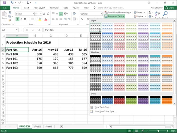
Figure 2-5: Selecting a format for the new data table in the Table Styles gallery.

As soon as you click one of the table formatting thumbnails in this Table Styles gallery, Excel makes its best guess as to the cell range of the data table to apply it to (indicated by the marquee around its perimeter), and the Format As Table dialog box similar to the one shown in Figure 2-6 appears.

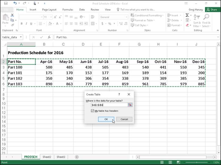
Figure 2-6: Indicating the range of the table in the Format As Table dialog box after selecting the style of table format.

This dialog box contains a Where Is the Data for Your Table? text box that shows the address of the cell range currently selected by the marquee and a My Table Has Headers check box (selected by default).

If Excel does not correctly guess the range of the data table you want to format, drag through the cell range to adjust the marquee and the range address in the Where Is the Data for Your Table? text box. If your data table doesn’t use column headers, click the My Table Has Headers check box to deselect it before you click the OK button — Excel will then add its own column headings (Column1, Column2, Column3, and so forth) as the top row of the new table.

Keep in mind that the table formats in the Table Styles gallery are not available if you select multiple nonadjacent cells before you click the Format as Table command button on the Home tab. You can convert only one range of cell data into a table at a time.

After you click the OK button in the Format As Table dialog box, Excel applies the format of the thumbnail you clicked in the gallery to the data table, and the command buttons on the Design tab of the Table Tools contextual tab appear on the Ribbon. (See Figure 2-7.)

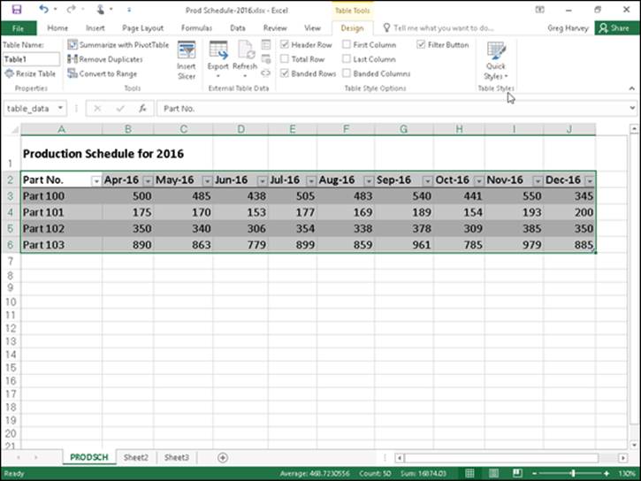
Figure 2-7: After you select an initial table format, the Design tab under Table Tools appears.

As you can see in Figure 2-7, when Excel defines a range as a table, it automatically adds AutoFilter drop-down buttons to each of the column headings (the little buttons with a triangle pointing downward in the lower-right corner of the cells with the column labels). To hide these AutoFilter buttons, click the Filter button on the Data tab or press Alt+AT. (You can always redisplay them by clicking the Filter button on the Data tab or by pressing Alt+AT a second time.)

The Design contextual tab enables you to use the Live Preview feature to see how your table data would appear in other table styles. Simply select the Quick Styles button and then highlight any of the format thumbnails in the Table Style group with the mouse or Touch pointer to see the data in your table appear in that table format, using the vertical scroll bar to scroll the styles in the Dark section into view in the gallery.

In addition to enabling you to select a new format from the Table gallery in the Table Styles group, the Design tab contains a Table Style Options group you can use to further customize the look of the selected format. The Table Style Options group contains the following check boxes:

· Header Row: Add Filter buttons to each of the column headings in the first row of the table.

· Total Row: Add a Total row to the bottom of the table that displays the sum of the last column of the table (assuming that it contains values). To apply a Statistical function other than Sum to the values in a particular column of the new Total row, click the cell in that column’s Total row. Doing this displays a drop-down list — None, Average, Count, Count Numbers, Max, Min, Sum, StdDev (Standard Deviation), or Var (Variation) — on which you click the new function to use.

· Banded Rows: Apply shading to every other row in the table.

· First Column: Display the row headings in the first row of the table in bold.

· Last Column: Display the row headings in the last row of the table in bold.

· Banded Columns: Apply shading to every other column in the table.

Keep in mind that whenever you assign a format in the Table Styles gallery to one of the data tables in your workbook, Excel automatically assigns that table a generic range name (Table1, Table2, and so on). You can use the Table Name text box in the Properties group on the Design tab to rename the data table by giving it a more descriptive range name.

When you finish selecting and/or customizing the formatting of your data table, click a cell outside of the table to remove the Design contextual tab from the Ribbon. If you later decide that you want to further experiment with the table’s formatting, click any of the table’s cells to redisplay the Design contextual tab at the end of the Ribbon.

Formatting Tables with the Quick Analysis Tool

You can use Excel’s handy Quick Analysis tool to quickly format your data as a new table. Simply select all the cells in the table, including the cells in the first row with the column headings. As soon as you do, the Quick Analysis tool appears in the lower-right corner of the cell selection (the outlined button with the lightning bolt striking the selected data icon). When you click this tool, the Quick Analysis options palette appears with five tabs (Formatting, Charts, Totals, Tables, and Sparklines).

Click the Tables tab in the Quick Analysis tool’s option palette to display its Table and Pivot Table buttons. When you highlight the Table button on the Tables tab, Excel’s Live Preview shows you how the selected data will appear formatted as a table. (See Figure 2-8.) To apply this previewed formatting and format the selected cell range as a table, you have only to click the Table button.

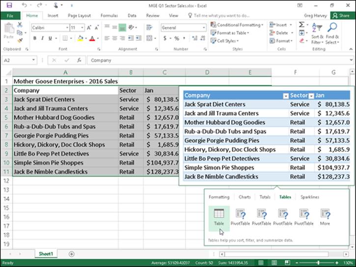
Figure 2-8: Previewing the selected data formatted as a table with the Quick Analysis tool.

As soon as you click the Table button, the Quick Analysis options palette disappears and the Design contextual table appears on the Ribbon. You can then use its Table Styles drop-down gallery to select a different formatting style for your table. (The Tables button on the Quick Analysis tool’s Tables tab offers only the one blue medium style shown in the Live Preview.)

Formatting Cells from the Ribbon

Some spreadsheet tables require a lighter touch than formatting as a table offers. For example, you may have a data table where the only emphasis you want to add is to make the column headings bold at the top of the table and to underline the row of totals at the bottom (done by drawing a borderline along the bottom of the cells).

The formatting buttons that appear in the Font, Alignment, and Number groups on the Home tab enable you to accomplish just this kind of targeted cell formatting. See Table 2-1 for a complete rundown on the use of each of these formatting buttons.

Table 2-1 The Formatting Command Buttons in the Font, Alignment, and Number Groups on the Home Tab

Don’t forget about the shortcut keys: Ctrl+B for toggling on and off bold in the cell selection, Ctrl+I for toggling on and off italics, and Ctrl+U for toggling on and off underlining for quickly adding or removing these attributes from the entries in the cell selection.

Formatting Cell Ranges with the Mini-Toolbar

Excel 2016 makes it easy to apply common formatting changes to a cell selection right within the Worksheet area thanks to its mini-toolbar feature — nicknamed the mini-bar.

To display the mini-toolbar, select the cells that need formatting and then right-click somewhere in the cell selection. The mini-toolbar then appears immediately below or above the cell selection’s shortcut menu. (See Figure 2-9.)

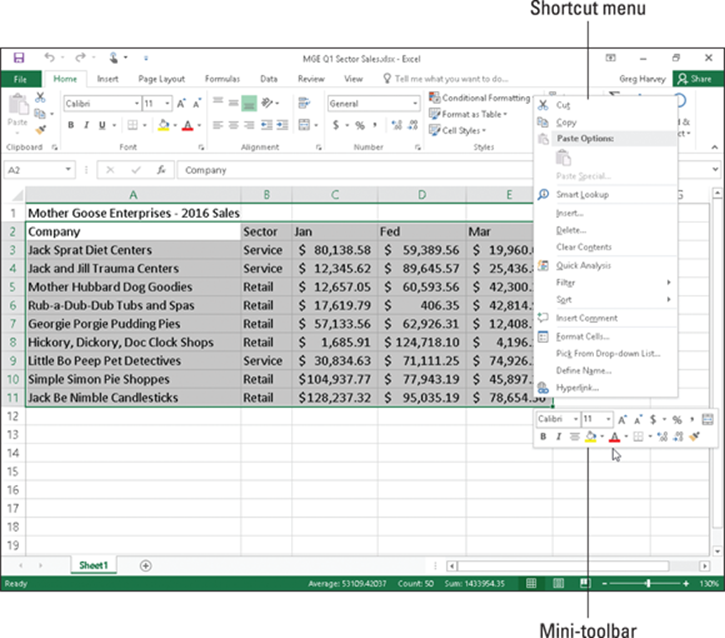
Figure 2-9: Right-click your cell selection to display its shortcut menu along with the mini-bar, whose buttons you can use to format the selection.

The mini-toolbar contains most of the buttons from the Font group of the Home tab (with the exception of the Underline button). It also contains the Center & Merge and Center buttons from the Alignment group (see “Altering the alignment” later in this chapter) and the Accounting Number Format, Percent Style, Comma Style, Increase Decimal, and Decrease Decimal buttons from the Number group. Simply click these buttons to apply their formatting to the current cell selection.

In addition, the mini-toolbar contains the Format Painter button from the Clipboard group of the Home tab, which you can use to copy the formatting in the active cell to a cell selection you make. (See “Hiring Out the Format Painter” later in this chapter for details.)

To display the mini-toolbar on a touchscreen device, tap and hold any cell in the selected range with your finger. Note that the mini-toolbar that appears is a little different from the one you see when you right-click a cell selection with a physical mouse. This one contains a single row of command buttons that combine editing and formatting functions — Paste, Cut, Copy, Clear, Fill Color, Font Color, and AutoFill followed by a Show Context Menu button (with a black triangle pointing downward). Tap the Show Context Menu button to display a pop-up menu of other editing and formatting options. Tap the Format Cells button on this menu to get access to all sorts of formatting options (see section that follows for details).

Note that if your device has a stylus, tapping and holding a cell in the selected cell range displays the standard mini-toolbar just as though you were using a mouse.

Using the Format Cells Dialog Box

Although the command buttons in the Font, Alignment, and Number groups on the Home tab give you immediate access to the most commonly used formatting commands, they do not represent all of Excel’s formatting commands by any stretch of the imagination.

To have access to all the formatting commands, you need to open the Format Cells dialog box either by clicking the Dialog Box launcher in the Number group on the Ribbon’s Home tab, choosing the More Number Formats option at the bottom of the Number Format button’s drop-down menu in the same Number group, or by simply pressing Ctrl+1.

The Format Cells dialog box contains six tabs: Number, Alignment, Font, Border, Fill, and Protection. (In this chapter, I show you how to use them all except the Protection tab; for information on that tab, see Book IV, Chapter 1.)

The keystroke shortcut that opens the Format Cells dialog box — Ctrl+1 — is one worth knowing. Just keep in mind that the keyboard shortcut is pressing the Ctrl key plus the number 1 key, and not the function key F1.

Assigning number formats

When you enter numbers in a cell or a formula that returns a number, Excel automatically applies the General number format to your entry. The General format displays numeric entries more or less as you enter them. However, the General format does make the following changes to your numeric entries:

· Drops any trailing zeros from decimal fractions so that 4.5 appears when you enter 4.500 in a cell.

· Drops any leading zeros in whole numbers so that 4567 appears when you enter 04567 in a cell.

· Inserts a zero before the decimal point in any decimal fraction without a whole number so that 0.123 appears when you enter .123 in a cell.

· Truncates decimal places in a number to display the whole numbers in a cell when the number contains too many digits to be displayed in the current column width. It also converts the number to scientific notation when the column width is too narrow to display all integers in the whole number.

Remember that you can always override the General number format when you enter a number by entering the characters used in recognized number formats. For example, to enter the value 2500 and assign it the Currency number format that displays two decimal places, you enter$2,500.00 in the cell.

Note that although you can override the General number format and assign one of the others to any numeric value that you enter into a cell, you can’t do this when you enter a formula into a cell. To apply another format to a calculated result, select its cell and then assign the Currency number format that displays two decimal places by clicking Accounting Number Format in the Number group on the Ribbon’s Home tab or by selecting Currency or Accounting on the Number tab of the Format Cells dialog box (Ctrl+1).

Using one of the predefined number formats

Any time you apply a number format to a cell selection (even if you do so with a command button in the Number group on the Ribbon’s Home tab instead of selecting the format from the Number tab of the Format Cells dialog box), you’re telling Excel to apply a particular group of format codes to those cells.

When you first open the Format Cells dialog box with a range of newly entered data selected, the General category of number formats is highlighted in the Category list box with the words “General format cells have no specific number format” showing in the area to the right. Directly above this cryptic message (which is Excel-speak for “We don’t care what you’ve put in your cell; we’re not changing it!”) is the Sample area. This area shows how the number in the active cell appears in whatever format you choose. (This is blank if the active cell is blank or if it contains text instead of a number.)

What you see is not always what you get

The number format that you assign to cells with numeric entries in the worksheet affects only the way they are displayed in their cells, and not their underlying values. For example, if a formula returns the value 3.456789 in a cell and you apply a number format that displays only two decimal places, Excel will display the value 3.46 in the cell. If you then refer to the cell in a formula that multiplies its value by 2, Excel returns the result 6.913578 instead of the result 6.92, which would be the result if Excel was actually multiplying 3.46 by 2. If you want to modify the underlying value in a cell, you use the ROUND function. (See Book III, Chapter 5 for details.)

When you click the Number, Currency, Accounting, or Percentage category in the Category list box, more options appear in the area just to the right of the Category list box in the form of different check boxes, list boxes, and spinner buttons. (Figure 2-10 shows the Format Cells dialog box when Currency is selected in the Category list box.) These options determine how you want items such as decimal places, dollar signs, comma separators, and negative numbers to be used in the format category that you’ve chosen.

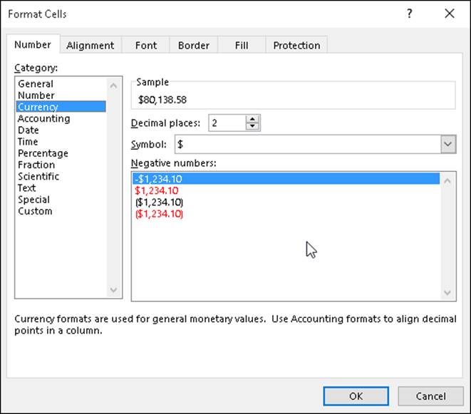
Figure 2-10: Options for customizing the formatting assigned by the Currency number format.

When you choose the Date, Time, Fraction, Special, or Custom category, a large Type list box appears that contains handfuls of predefined category types, which you can apply to your value to change its appearance. Just like when you’re selecting different formatting categories, the Sample area of the Format Cells dialog box shows you how the various category types will affect your selection.

I should note here that Excel always tries to choose an appropriate format category in the Category list box based on the way you entered your value in the selected cell. If you enter 3:00 in a cell and then open the Number tab of the Format Cells dialog box (Ctrl+1), Excel highlights the h:mm time format in the Custom category in the Type list box.

Deciphering the Custom number formats

You probably noticed while playing around selecting different formats in the Category list box that, for the most part, the different categories and their types are pretty easy — if not a breeze — to comprehend. For most people, that self-assured feeling goes right out the window as soon as they click the Custom category and get a load of its accompanying Type list box, shown in Figure 2-11. It starts off with the nice word General, then 0, then 0.00, and after that, all hell breaks loose! Codes with 0s and #s (and other junk) start to appear, and it only goes downhill from there.

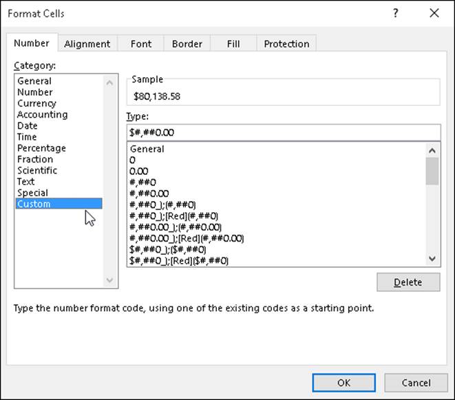
Figure 2-11: Creating your own number format using the Custom category in the Format Cells dialog box.

As you move down the list, the longer codes are divided into sections separated by semicolons and enclosed within square brackets. Although at first glance these codes appear as gibberish, you’ll actually find that they’re quite understandable. (Well, would you believe useful, then?)

And these codes can be useful, especially after you understand them. You can use them to create number formats of your own design. The basic keys to understanding number format codes are as follows:

· Excel number formats use a combination of 0, ?, and # symbols with such punctuation as dollar signs, percent signs, and commas to stand for the formatted digits in the numbers that you format.

· The 0 is used to indicate how many decimal places (if any) are allowed in the format. The format code 0.00 indicates that two decimal places are used in the number. The format code 0 alone indicates that no decimal places appear. (The display of all values is rounded up to whole numbers.)

· The ? is used like the 0 except that it inserts spaces at the end as needed to make sure that values line up on the decimal point. For example, by entering the number format 0.??, such values as 10.5 and 24.71 line up with each other in their cells because Excel adds an extra space after the 5 to push it over to the left so that it’s in line with the 7 of 71. If you used the number format 0.00 instead, these two values would not line up on the decimal point when they are right-aligned in their cells.

· The # symbol is used with a comma to indicate that you want thousands, hundred thousands, millions, zillions, and so on in your numbers, with each group of three digits to be separated with a comma.

· The $ (dollar sign) symbol is added to the beginning of a number format if you want dollar signs to appear at the beginning of every formatted number.

· The % (percent sign) symbol is added to the end of the number format if you want Excel to actually transform the value into a percentage (multiplying it by 100 and adding a percent sign).

Number formats can specify one format for positive values, another for negative values, a third for zero values, and even a fourth format for text in the cells. In such complex formats, the format codes for positive values come first, followed by the codes for negative values, and a semicolon separates each group of codes. Any format codes for how to handle zeros and text in a cell come third and fourth, respectively, in the number format, again separated by semicolons. If the number format doesn’t specify special formatting for negative or zero values, these values are automatically formatted like positive values. If the number format doesn’t specify what to do with text, text is formatted according to Excel’s default values. For example, look at the following number format:

#,##0_);(#,##0)

This particular number format specifies how to format positive values (the codes in front of the semicolon) and negative values (the codes after the semicolon). Because no further groups of codes exist, zeros are formatted like positive values, and no special formatting is applied to text.

If a number format puts negative values inside parentheses, the positive number format portion often pads the positive values with a space that is the same width as a right parenthesis. To indicate this, you add an underscore (by pressing Shift and the hyphen key) followed immediately by a closed parenthesis symbol. By padding positive numbers with a space equivalent to a right parenthesis, you ensure that digits of both positive and negative values line up in a column of cells.

You can assign different colors to a number format. For example, you can create a format that displays the values in green (the color of money!) by adding the code [GREEN] at the beginning of the format. A more common use of color is to display just the negative numbers in red (ergo the saying “in the red”) by inserting the code [RED] right after the semicolon separating the format for positive numbers from the one for negative numbers. Color codes include [BLACK], [BLUE], [CYAN], [GREEN], [MAGENTA], [RED], [WHITE], and [YELLOW].

Date number formats use a series of abbreviations for month, day, and year that are separated by characters, such as a dash (—) or a slash (/). The code m inserts the month as a number; mmm inserts the month as a three-letter abbreviation, such as Apr or Oct; and mmmm spells out the entire month, such as April or October. The code d inserts the date as a number; dd inserts the date as a number with a leading zero, such as 04 or 07; ddd inserts the date as a three-letter abbreviation of the day of the week, such as Mon or Tue; and dddd inserts the full name of the day of the week, such as Monday or Tuesday. The code yy inserts the last two digits of the year, such as 05 or 07; yyyy inserts all four digits of the year, such as 2005, 2007, and so on.

Time number formats use a series of abbreviations for the hour, minutes, and seconds. The code h inserts the number of the hour; hh inserts the number of the hour with leading zeros, such as 02 or 06. The code m inserts the minutes; the code mm inserts the minutes with leading zeros, such as 01 or 09. The code s inserts the number of seconds; ss inserts the seconds with leading zeros, such as 03 or 08. Add AM/PM or am/pm to have Excel tell time on a 12-hour clock, and add either AM (or am) or PM (or pm) to the time number depending on whether the date is before or after noon. Without these AM/PM codes, Excel displays the time number on a 24-hour clock, just like the military does. (For example, 2:00 PM on a 12-hour clock is expressed as 14:00 on a 24-hour clock.)

So that’s all you really need to know about making some sense of all those strange format codes that you see when you select the Custom category on the Number tab of the Format Cells dialog box.

Designing your own number formats

Armed with a little knowledge on the whys and wherefores of interpreting Excel number format codes, you are ready to see how to use these codes to create your own custom number formats. The reason for going through all that code business is that, in order to create a custom number format, you have to type in your own codes.

To create a custom format, follow this series of steps:

1. Open a worksheet and enter a sample of the values or text to which you will be applying the custom format.

If possible, apply the closest existing format to the sample value as you enter it in its cell. (For example, if you’re creating a derivative of a Currency format, enter it with the dollar sign, commas, and decimal points that you know you’ll want in the custom format.)

2. Open the Format Cells dialog box and use its categories to apply the closest existing number format to the sample cell.

3. Select Custom in the Category list box and then edit the codes applied by the existing number format that you chose in the Type list box until the value in the Sample section appears exactly as you want it.

What could be simpler? Ah, but Step 3, there’s the rub: editing weird format codes and getting them just right so that they produce exactly the kind of number formatting that you’re looking for!

Actually, creating your own number format isn’t as bad as it first sounds, because you “cheat” by selecting a number format that uses as many of the codes as possible that you need in the new custom number that you’re creating. Then you use the Sample area to keep a careful eye on the results as you edit the codes in the existing number format. For example, suppose that you want to create a custom date format to use on the current date that you enter with Excel’s built-in NOW function. (See Book III, Chapter 3 for details.) You want this date format to display the full name of the current month (January, February, and so on), followed by two digits for the date and four digits for the year, such as November 06, 2016.

To do this, use the Function Wizard to insert the current date into a worksheet cell; then with this cell selected, open the Format Cells dialog box and scroll down through the Custom category Type list box on the Number tab until you see the date codes m/d/yyyy h:mm. Highlight these codes and then edit them as follows in the Type text box directly above:

mmmm dd, yyyy

The mmmm format code inserts the full name of the month in the custom format; dd inserts two digits for the day (including a leading zero, like 02 and 03); the yyyy code inserts the year. The other elements in this custom format are the space between the mmmm and dd codes and a comma and a space between the dd and yyyy codes (these being purely “punctuational” considerations in the custom format).

What if you want to do something even fancier and create a custom format that tells you something like “Today is Sunday, November 06, 2016” when you format a cell containing the NOW function? Well, you select your first custom format and add a little bit to the front of it, as follows:

"Today is" dddd, mmmm dd, yyyy

In this custom format, you’ve added two more elements: Today is and dddd. The Today is code tells Excel to enter the text between the quotation marks verbatim; the dddd code tells the program to insert the whole name of the day of the week. And you thought this was going to be a hard section!

Next, suppose that you want to create a really colorful number format — one that displays positive values in blue, negative values in red (what else?), zero values in green, and text in cyan. Further suppose that you want commas to separate groups of thousands in the values, no decimal places to appear (whole numbers only, please), and negative values to appear inside parentheses (instead of using that tiny little minus sign at the start). Sound complex? Hah, this is a piece of cake.

Take four blank cells in a new worksheet and enter 1200 in the first cell, -8000 in the second cell, 0 in the third cell, and the text Hello There! in the fourth cell. Then select all four cells as a range (starting with the one containing 1200 as the first cell of the range). Open the Format Cells dialog box and select the Number tab and Number in the Category list. Then select the #,##0_);[Red](#,##0) code in the Custom category Type list box (it’s the seventh set down from the top of the list box) and edit it as follows:

[Blue]#,##0_);[Red](#,##0);[Green];[Cyan]

Click OK. That’s all there is to that. When you return to the worksheet, the cell with 1200 appears in blue as 1,200, the -8000 appears in red as (8,000), the 0 appears in green, and the text “Hello There!” appears in a lovely cyan.

Before you move on, you should know about a particular custom format because it can come in really handy from time to time. I’m referring to the custom format that hides whatever has been entered in the cells. You can use this custom format to temporarily mask the display of confidential information used in calculating the worksheet before you print and distribute the worksheet. This custom format provides an easy way to avoid distributing confidential and sensitive information while protecting the integrity of the worksheet calculations at the same time.

To create a custom format that masks the display of the data in a cell selection, you simply create an “empty” format that contains just the semicolon separators in a row:

;;;

This is one custom format that you can probably type by yourself!

After creating this format, you can blank out a range of cells simply by selecting them and then selecting this three-semicolon custom format in the Format Cells dialog box. To bring back a cell range that’s been blanked out with this custom format, simply select what now looks like blank cells and then select one of the other (visible) formats that are available. If the cell range contains text and values that normally should use a variety of different formats, first use General to make them visible. After the contents are back on display, format the cells in smaller groups or individually, as required.

Altering the alignment

You can use Excel’s Alignment options by using command buttons in the Alignment group of the Ribbon’s Home tab and by using options on the Alignment tab of the Format Cells dialog box to change the way cell entries are displayed within their cells.

Alignment refers to both the horizontal and vertical placement of the characters in an entry with regard to its cell boundaries as well as the orientation of the characters and how they are read. Horizontally, Excel automatically right-aligns all numeric entries and left-aligns all text entries in their cells (referred to as General alignment). Vertically, Excel aligns all types of cell entries with the bottom of their cells.

In the Horizontal drop-down list on the Alignment tab of the Format Cells dialog box, Excel offers you the following horizontal text alignment choices:

· General (the default) right-aligns a numeric entry and left-aligns a text entry in its cell.

· Left (Indent) left-aligns the entry in its cell and indents the characters from the left edge of the cell by the number of characters entered in the Indent combo box (which is 0 by default).

· Center centers any type of cell entry in its cell.

· Right (Indent) right-aligns the entry in its cell and indents the characters from the right edge of the cell by the number of characters entered in the Indent combo box (which is 0 by default).

· Fill repeats the entry until its characters fill the entire cell display. When you use this option, Excel automatically increases or decreases the repetitions of the characters in the cell as you adjust the width of its column.

· Justify spreads out a text entry with spaces so that the text is aligned with the left and right edges of its cell. If necessary to justify the text, Excel automatically wraps the text onto more than one line in the cell and increases the height of its row. If you use the Justify option on numbers, Excel left-aligns the values in their cells just as if you had selected the Left align option.

· Center Across Selection centers a text entry over selected blank cells in columns to the right of the cell entry.

· Distributed (Indent) indents the text in from the left and right cell margins by the amount you enter in the Indent text box or select with its spinner buttons (which appear when you select this option from the Horizontal drop-down list) and then distributes the text evenly in the space in between.

For text entries in the worksheet, you can also add the Wrap Text check box option to any of the horizontal alignment choices. (Note that you can also access this option by clicking the Wrap Text button in the Alignment group of the Home tab on the Ribbon.) When you select the Wrap Text option, Excel automatically wraps the text entry to multiple lines within its cells while maintaining the type of alignment that you’ve selected (something that automatically happens when you select the Justify alignment option).

Instead of wrapping text that naturally increases the row height to accommodate the additional lines, you can use the Shrink to Fit check box option on the Alignment tab of the Format Cells dialog box to have Excel reduce the size of the text in the cell sufficiently so that all its characters fit within their current column widths.

In addition, Excel offers the following vertical text alignment options from the Vertical drop-down list:

· Top (the default) aligns any type of cell entry with the top edge of its cell.

· Center centers any type of cell entry between the top and bottom edges of its cell.

· Bottom aligns any type of cell entry with the bottom edge of its cell.

· Justify wraps the text of a cell entry on different lines spread out with blank space so that they are vertically aligned between the top and bottom edges of the cell.

· Distributed wraps the text of the cell entry on different lines distributed evenly between the top and bottom edges of its cell.

Finally, as part of its alignment options, Excel lets you alter the orientation (the angle of the characters in an entry in its cell) and text direction (the way the characters are read). The direction is left-to-right for European languages and right-to-left for some languages, such as Hebrew and Arabic. (Chinese characters can also sometimes be read from right to left, as well.)

Wrapping text entries to new lines in their cells

You can use the Wrap Text button on the Ribbon’s Home tab or the Wrap Text check box in the Text Control section of the Alignment tab to have Excel create a multi-line entry from a long text entry that would otherwise spill over to blank cells to the right. In creating a multi-line entry in a cell, the program also automatically increases the height of its row if that is required to display all the text.

To get an idea of how text wrap works in cells, compare Figures 2-12 and 2-13. Figure 2-12 shows you a row of long text entries that spill over to succeeding blank cells in columns to the right. Figure 2-13 shows you these same entries after they have been formatted with the Wrap Text option. The first long text entry is in cell A8 and the last in cell I8. They all use General alignment (same as Left for text) with the Wrap Text option.

Figure 2-12: Worksheet with long text entries that spill over into blank cells on the right.

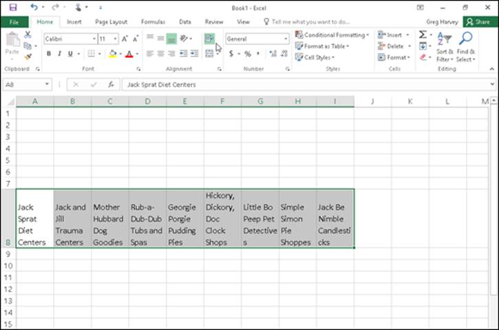
Figure 2-13: Worksheet after wrapping long text entries in their cells, increasing the height of their rows.

When you create multi-line text entries with the Wrap Text option, you can decide where each line breaks by inserting a new paragraph. To do this, you put Excel in Edit mode by clicking the insertion point in the Formula bar at the place where a new line should start and pressing Alt+Enter. When you press the Enter key to return to Ready mode, Excel inserts an invisible paragraph marker at the insertion point that starts a new line both on the Formula bar and within the cell with the wrapped text.

If you ever want to remove the paragraph marker and rejoin text split on different lines, click the insertion point at the beginning of the line that you want to join on the Formula bar and press the Backspace key.

Reorienting your entries

Excel makes it easy to change the orientation (that is, the angle of the baseline on which the characters rest) of the characters in a cell entry by rotating up or down the baseline of the characters.

The Orientation command button in the Alignment group on the Ribbon’s Home tab contains the following options on its drop-down menu:

· Angle Counterclockwise rotates the text in the cell selection up 45 degrees from the baseline.

· Angle Clockwise rotates the text in the cell selection down 45 degrees from the baseline.

· Vertical Text aligns the text in the cell selection in a column where one letter appears over the other.

· Rotate Text Up rotates the text in the cell selection up 90 degrees from the baseline.

· Rotate Text Down rotates the text in the cell selection down 90 degrees from the baseline.

· Format Cell Alignment opens the Alignment tab on the Format Cells dialog box.

You can also alter the orientation of text in the cell selection on the Alignment tab of the Format Cells dialog box (Ctrl+1) using the following options in its Orientation area:

· Enter the value of the angle of rotation for the new orientation in the Degrees text box or click the spinner buttons to select this angle. Enter a positive value (such as 45) to have the characters angled above the normal 90-degree line of orientation and a negative value (such as -45) to have them angled above this line.

· Click the point on the sample Text box on the right side of the Orientation area that corresponds to the angle of rotation that you want for the characters in the selected cells.

· Click the sample Text box on the left side of the Orientation area to have the characters stacked one on top of the other (as shown in the orientation of the word “Text” in this sample box).

After changing the orientation of entries in a selection, Excel automatically adjusts the height of the rows in the cell selection to accommodate the rotation up or down of the cell entries. Figure 2-14 shows the top part of a worksheet after rotating the column headings for a new data table up 90 degrees. Note how Excel increased the height of row 10 to accommodate this change.

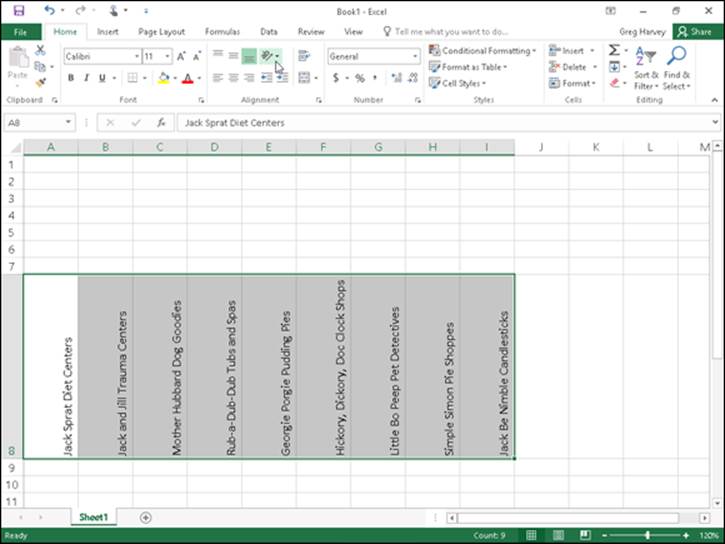
Figure 2-14: Worksheet after rotating a table’s column headings up 90 degrees.

Fancy fonts and colors

You can assign any of the fonts that you’ve installed for your printer to cells in a worksheet. Along with selecting a new font (also known as a typeface), you can choose a new font size (in points), assign a font style (such as bold, italic, underline, or strikethrough), as well as change the color of the font.

Note that you can always tell the font and font size of the cell entry in the active cell by looking at the font name displayed in the Font combo box and the point size displayed in the Font Size combo box in the Font group on the Home tab of the Ribbon. You can also tell which, if any, text attributes are assigned to the entry by looking at the Bold, Italic, and Underline buttons in this group. Excel indicates which of these attributes have been assigned to the cell by highlighting the B, I, or U button in the standard beige highlight color.

Selecting fonts and colors from the Ribbon

You can change the font, font size, font style, and font color using the command buttons in the Font group on the Home tab of the Ribbon. The only aspects you can’t change or assign are the type of the underlining (besides single or double) and special font styles including strikethrough, superscript, and subscript.

To change the font with the command buttons in the Font group on the Ribbon’s Home tab, select the cell, cell range, or nonadjacent selection to which you want to assign the new font, size, style, or color, and then do one of the following:

· To assign a new font to the selection, click the Font drop-down button and then select the font from the drop-down list.

· To assign a new point size to the selection, click the Font Size drop-down button and then select the size from the drop-down list. (You can also do this by clicking the Font text box, typing the point size, and pressing Enter.)

· To increase the font size a single point at a time, click the Increase Font Size button.

· To decrease the font size a single point at a time, click the Decrease Font Size button.

· To assign a new font style to a selection, click the appropriate tool in the Formatting toolbar: Click the Bold button (the one with B) to bold the selection, the Italic button (the one with I) to italicize the selection, and the Underline button (the one with the U) to underline the selection. To assign double underlining to the cell selection, click the drop-down button attached to the Underline button and then choose Double Underline from its drop-down menu.

· To assign a new font color, click the Font Color pop-up button and then click the new color in the drop-down palette.

Live Preview enables you to see how the cell selection looks in a font or font size that you highlight on the Font or Font Size drop-down list — provided, of course, that the selection in the columns and rows is not obscured when these drop-down lists are displayed.

Note that you can immediately remove any font change that you make by clicking the Undo button on the Quick Access toolbar (or by pressing Ctrl+Z). You can also remove boldface, italics, and underlining assigned to a cell selection by clicking the appropriate button (Bold, Italic, and Underline) on the Formatting toolbar. This action removes the shading that outlines the button’s B, I, or U icon.

Selecting fonts and colors in the Format Cells dialog box

You can also select a new font, font size, font style, and font color for your selection on the Font tab of the Format Cells dialog box (Ctrl+1). Figure 2-15 shows the Font tab of the Format Cells dialog box that appears when an empty cell that uses the Normal style is active. In this figure, the current Font is Calibri (Body), the Font Style is Regular, the Font Size is 11 (points), the Underline is None, and the Color is Automatic.

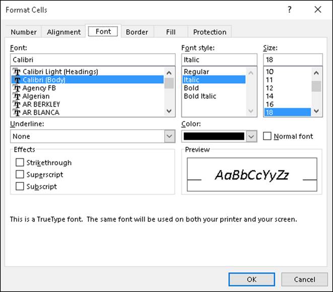
Figure 2-15: You can assign new fonts, font sizes, attributes, and colors on the Font tab of the Format Cells dialog box.

To select a new font color from the Font Color drop-down palette in the Font group on the Ribbon’s Home tab or from the Color drop-down palette on the Font tab of the Format Cells dialog box, click its drop-down button. Both drop-down palettes contain color swatches arranged in two groups: Theme colors to select one of the colors used in Excel’s themes (see Book V, Chapter 2) and Standard colors to select one of the primary Windows colors. To select a font color from either of these two groups, click its color swatch.

If none of the preset colors will do, click the More Colors option at the bottom of the drop-down palette to open the Colors dialog box. This dialog box contains a Standard tab where you can select a new color by clicking its hexagram swatch in the color honeycomb or shade of gray hexagram below. The Custom tab enables you to select a custom color by changing the RGB (Red, Green, and Blue) or HSL (Hue, Saturation, and Luminosity) values. You can do this either by dragging through the color grid and tint slider at the top of the Custom tab or by entering new values in the Red, Green, and Blue (when the RGB Color Model is selected) or the Hue, Sat, and Lum (when the HSL Color Model is selected) text boxes below or by selecting them with their spinner buttons.

Note that Excel adds a swatch for each custom color you select or define to a Recent Colors section that then appears on both the Font Color and Fill Color buttons’ drop-down palettes, making it easy to apply these custom colors to the text and fills of other cells in the worksheet.

Changing the Automatic color in Windows 7

When running Excel 2016 under Windows 7, you can change the Automatic color from the default of black to some other color. To do this, you open the Window Color and Appearance dialog box by right-clicking the Windows 7 desktop and then choosing Personalize from the shortcut menu; click the Window Color button and then click the Advanced Appearance Settings link.

In the Window Color and Appearance dialog box, select Window at the very bottom of the Item drop-down list and then click a new color on the Color drop-down palette in the last row (opposite Font) immediately above the OK and Cancel buttons. Click OK.

Basic borders, fills, and patterns

Excel makes it easy to add borders as well as to assign new background fill colors, gradients, and shading patterns to cells in the worksheet. You can use the borders to outline tables of data — particularly important cells — or to underscore rows of key data. You can also apply various color gradients and shading patterns to cells to draw attention to significant aspects of the spreadsheet.

When adding borders and shading, you can make your job a great deal easier by removing the gridlines used in the Worksheet area to indicate the borders of the cells in the worksheet. To remove these gridlines, deselect the Gridlines check box on the View tab of the Ribbon (or press Alt+WVG) to remove its check mark. After you’ve dispensed with a worksheet’s gridlines, you can immediately tell whether you’ve added the kind of borders that you want and better judge the effect of the color and shading changes that you make.

Note that removing the display of the gridlines in the Workbook window has no effect on the appearance of gridlines in a printed copy of the spreadsheet. If you turn on gridlines for a printout by selecting the Print check box in the Gridlines column of the Sheet Options group on the Page Layout tab (or press Alt+PPG), Excel prints these lines on the printed version of the worksheet even when they do not appear onscreen.

Right on the borderline

When applying borderlines to a cell selection, you have a choice between using the options on the drop-down menu that’s attached to the Borders button in the Font group on the Home tab and using the options on the Border tab of the Format Cells dialog box. You can compare the options offered by each in Figures 2-16 and 2-17. Figure 2-16 shows the border options on the drop-down menu, and Figure 2-17 shows the options on the Border tab of the Format Cells dialog box.

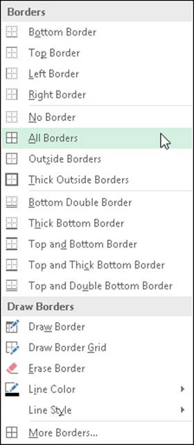
Figure 2-16: The border options available on the Home tab’s Borders button’s drop-down menu.

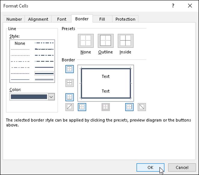
Figure 2-17: The border options available on the Border tab of the Format Cells dialog box.

To apply borders to the cell selection by using the options on the Borders button’s drop-down menu, choose the option on the menu with the type of border you want drawn. To remove a borderline that you select in error, simply choose the No Border option at the top of this drop-down menu.

While defining the borderlines to apply in the Border tab, you can select a new style for the borderlines by clicking the Line style in the Style sample area. To select a new color (besides boring old black) for the borderlines that you’re about to apply, click the swatch of the new color you want to use in the Color drop-down palette.

When using the Borders palettes to assign borderlines to a cell selection, your options are limited to just the Border buttons displayed on the palette. This means that you don’t have as much choice in terms of line style and type of borderlines. (In other words, you can’t be applying any dashed diagonal borderlines from this palette.) You also can’t change the color of the borderlines from the Borders palette.

Keep in mind that the Borders button’s drop-down menu includes a couple of options that enable you to literally draw borders around a cell selection in your worksheet by dragging the mouse pointer through the cells. Choose the Draw Border option to draw a border just outlining the cells you select or Draw Border Grid to draw borders around each and every cell you select with the mouse.

To get rid of borderlines that you’ve added to a cell range, no matter which method you used to add them, select the range and then choose the No Border option from the Borders button’s drop-down menu.

Fun fills, great-looking gradients, and pretty patterns

In Excel 2016, you can not only select new background colors (referred to as fill colors) for the cell selection but you can also assign gradients (fills that gradually go from one color to another) and new dotted and crosshatched patterns to them.

When simply assigning a new fill color to the current cell selection, you can do this either by clicking a new color swatch on the Fill Color button’s drop-down palette (located in the Font group on the Ribbon’s Home tab) or by clicking the swatch in the Background Color area of the Fill tab in the Format Cells dialog box (Ctrl+1) shown in Figure 2-18.

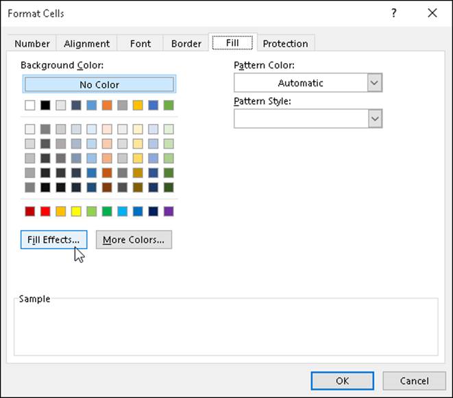
Figure 2-18: Using the options on the Fill tab to select a new fill color, gradient, or shading pattern for your cell selection.

· To assign a gradient to the cell selection, click the Fill Effects button to open the Fill Effects dialog box. (See Figure 2-19.) Select the beginning gradient color by clicking its swatch on the Color 1 drop-down color palette and the ending gradient color by clicking its swatch on the Color 2 drop-down palette. Note that you can then further refine the gradient by selecting a new shading style option button that determines the direction of the gradient pattern before you click OK.

· To add a dotted or crosshatched shading pattern to the cell selection (instead of a gradient — they don’t go together), click the pattern square on the Pattern Style’s drop-down palette. To change the color of the shading pattern (which is by default the black Automatic color), click a color swatch on the Pattern Color’s drop-down palette.

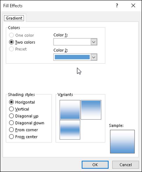
Figure 2-19: Selecting a new gradient for your cell selection in the Fill Effects dialog box.

Check the Sample area at the bottom of the Fill tab of the Format Cells dialog box to check out the shading pattern and make sure that it’s the one you want to use before you click OK to apply it to the cell selection. If you don’t like the effect after you’ve applied it to the cell selection, click the Undo button on the Quick Access toolbar or press Ctrl+Z immediately to remove it.

To get rid of all fill colors, gradients, and shading patterns used in a cell selection, click the No Fill option at the bottom of the Fill Color button’s drop-down palette on the Home tab.

Hiring Out the Format Painter

The Format Painter button (with paintbrush icon) in the Clipboard group of the Home tab takes formatting from the current cell and applies it to cells that you “paint” by dragging its special thick-white cross-plus-paintbrush mouse pointer through them. This tool, therefore, provides a quick-and-easy way to take a bunch of different formats (such as a new font, font size, bold, and italics) that you applied individually to a cell in the spreadsheet and then turn around and use them as the guide for formatting a new range of cells.

To use the Format Painter, follow these steps:

1. Position the cell cursor in a cell that contains the formatting that you want copied to another range of cells in the spreadsheet.

This cell becomes the sample cell whose formatting is taken up by Format Painter and copied in the cells that “paint” with its special mouse pointer.

2. Click the Format Painter button (with the paintbrush icon) in the Clipboard group on the Home tab of the Ribbon.

As soon as you click this button, Excel adds a paintbrush icon to the standard thick white-cross mouse pointer, indicating that the Format Painter is ready to copy the formatting from the sample cell.

3. Drag the mouse pointer through the range of cells that you want formatted identically to the sample cell.

The moment that you release the mouse button, the cells in the range that you just selected with the Format Painter become formatted the same way as the sample cell.

Normally, using the Format Painter is a one-shot deal because as soon as you release the mouse button after selecting a range of cells with the Format Painter, it turns off, and the mouse pointer reverts back to its normal function of just selecting cells in the worksheet (indicated by the return of the regular thick white-cross icon). If you ever want to keep the Format Painter turned on so that you can use it to format more than one range of cells in the worksheet, you need to double-click the Format Painter button on the Home tab instead of just single-clicking it. When you do this, the Format Painter button remains depressed (indicated by the shading) on the Home tab until you click its command button again. During this time, you can “paint” as many different cell ranges in the worksheet as you desire.

Using Cell Styles

Cell styles combine a number of different formatting aspects that can include number format, text alignment, font and font size, borders, fills, and protection status. (See Book IV, Chapter 1.)

In Excel 2016, cell styles really come alive in the form of the Cell Styles gallery that you open by clicking the Cell Styles button in the Styles group on the Ribbon’s Home tab.

The Cell Styles gallery contains loads of ready-made styles you can immediately apply to the current cell selection. These predefined cell styles are arranged into various sections: Good, Bad, and Neutral; Data and Model; Titles and Headings; Themed Cell Styles; and Number Format. (See Figure 2-20.)

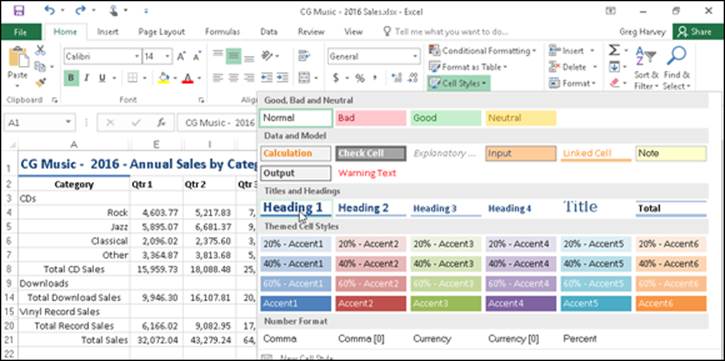
Figure 2-20: Selecting a new style for a cell selection from the Cell Styles gallery.

To apply one of the styles on the Cell Styles gallery, simply click the thumbnail of the desired style in the gallery after using the Live Preview feature to determine which style looks best on the data in your cell selection.

Using the Number Format cell styles

The Number Format section near the bottom of the Cell Styles gallery (see Figure 2-20) contains the following five predefined styles that you can use to format the values entered into the cell selection as follows:

· Comma sets the number format to the Comma Style (same as clicking the Comma Style command button in the Number group of the Home tab).

· Comma (0) sets the number format to the Comma Style format without any decimal places.

· Currency sets the number format to the Currency style format (same as clicking the Accounting Number Format command button in the Number group of the Home tab).

· Currency (0) sets the number format to the Currency style format without any decimal places (making your financial figures all dollars and no cents).

· Percent sets the number format to Percent style (same as clicking the Percent Style command button in the Number group of the Home tab).

You can combine the number formatting assigned from one of the Number Format cell styles with the other cell formatting assigned by the cell styles in the other three cell style groups: the Good, Bad, and Neutral (except for Normal, which applies the General number format); Data and Model; and Themed Cell Styles. To do this, however, assign the number formatting by clicking its style in the Number Format section of the Cell Styles gallery before you assign the other formatting by clicking its style in one of the other three sections of the Cell Styles gallery.

Click Normal, the first style in the Good, Bad, and Neutral section, in the Cell Styles gallery to return the formatting in the cell selection to its original state: General number format, left or right (depending on the contents), horizontal and bottom vertical alignment, Calibri (body), 11-point font size (unless you’ve changed the default font and size), no borders, no fill, and locked protection status.

Defining a custom cell style by example

You don’t have to live with just the predefined styles that Excel gives you on the Cell Styles gallery because you can readily create custom cell styles of your own.

By far the easiest way to create a new custom cell style is by example. When you create a cell style by example, you choose a cell that already displays all the formatting attributes (applied separately using the techniques discussed previously in this chapter) that you want included in the new cell style. Then, you follow these simple steps to create the new style by using the formatting in the sample cell:

1. Position the cell pointer in the cell with the formatting that you want in the new style.

2. Click the New Cell Style option at the bottom of the Cell Styles drop-down gallery (opened by clicking the Cell Styles button in the Styles group on the Ribbon’s Home tab).

This action opens the Style dialog box with a generic style name (Style 1, Style 2, and so on), and the formatting attributes applied to the cell are listed in the Style Includes (By Example) section of the dialog box.

3. Type the name for the new style in the Style Name text box (replacing the Style 1, Style 2, generic style name).

4. Click OK to close the Style dialog box.

When defining a style by example, select only one cell that you know contains all the formatting characteristics that you want in the new style. This way, you avoid the potential problem of selecting cells that don’t share the same formatting. If you select cells that use different formatting when defining a style by example, the new style will contain only the formatting that all cells share in common.

After you close the Style dialog box, Excel adds a thumbnail for the new style to a Custom section at the top of the Cell Styles gallery. To apply this new custom cell style to other cell selections in the worksheet, all you have to do is click its thumbnail in the Custom section of the gallery.

Creating a new cell style from scratch

You can also create a custom cell style from scratch by defining each of its formatting characteristics in the Style dialog box as follows:

1. Position the cell pointer in a cell that doesn’t have only the Excel default formatting applied to it and then click the New Cell Style option at the bottom of the Cell Styles drop-down gallery (opened by clicking the Cell Styles button in the Styles group on the Ribbon’s Home tab).

This action opens the Style dialog box with a generic style name (Style 1, Style 2, and so on), and with the attributes for the Normal style listed in the Style Includes (By Example) section of the dialog box.

2. Type a name for the new style that you are defining in the Style Name text box (replacing Style 1, Style 2, generic style name).

Now you need to select the formatting settings for the new style.

3. (Optional) Remove the check mark from the check box for any attribute (Number, Alignment, Font, Border, Fill, or Protection) that you don’t want included in the new style.

They are all selected by default.

4. Click the Format button in the Style dialog box.

This action opens the standard Format Cells dialog box, where you can use the options on its six tabs (Number, Alignment, Font, Border, Fill, and Protection) to select all the formatting attributes that you do want used when you apply the new style to a cell selection.

5. After you finish assigning the formatting attributes that you want in the new style in the Format Cells dialog box, click OK to return to the Style dialog box.

The Style Includes (By Example) section now lists all the attributes that you assigned in the Format Cells dialog box.

6. Click OK to close the Style dialog box.

As soon as you click OK, Excel applies the formatting in your newly defined custom style to the current cell and adds the new style to the Custom section of the Cell Styles gallery. To apply this new custom cell style to other cell selections in the worksheet, all you have to do is click its thumbnail in the Custom section of the gallery.

To remove a custom style from the Cell Styles gallery that you’ve defined by example or from scratch, you have to right-click its thumbnail in the gallery and then click Delete on its shortcut menu.

Merging styles into other workbooks

All custom cell styles that you create are saved, along with the data and formatting in the worksheet, when you save the file. The only styles, however, that are available when you begin a new worksheet are those predefined styles provided by Excel.

If you’ve created custom styles in another workbook that you want to use in a new workbook or in an existing one that you’ve opened for editing, you have to merge them into that workbook as follows:

1. Open the workbook file containing the custom styles that you want to copy and use.

You must have the workbook containing the custom styles to merge open, along with the workbook into which these custom styles will be copied.

2. Click the button on the Windows taskbar for the workbook file into which the custom styles will be merged.

This action makes the workbook into which the custom styles are to be copied the active one.

3. Click the Merge Styles option at the bottom of the Cell Styles drop-down gallery (opened by clicking the Cell Styles button in the Styles group on the Ribbon’s Home tab).

Excel opens the Merge Styles dialog box with a list box that displays the filenames of the all the workbooks that currently open in the program.

4. Click the name of the workbook that contains the custom styles you want merged into the active workbook and then click OK.

This action closes the Merge Styles dialog box. If the worksheet file that you selected contains custom styles with the same names as the custom styles defined in the active worksheet, Excel displays an alert box that asks whether you want to merge the styles that have the same names. Click Yes to replace all styles in the active workbook with those that have the same name in the workbook file that you’re copying from. Click No if you don’t want the styles in the active workbook to be overwritten, in which case Excel merges the styles with unique names from the other worksheet.

After merging styles from another open workbook, you can close that workbook by clicking its button on the Windows taskbar and then clicking its Close Window. You can then begin applying the merged custom styles, which now appear in the Custom section at the top of the Cell Styles gallery, to cell selections by clicking their thumbnails in the gallery.

Conditional Formatting

Excel 2016’s Conditional Formatting feature enables you to format a range of values so that unusual or unwanted values, or values outside certain limits, are automatically formatted in such a way as to call attention to them.

When you click the Conditional Formatting button in the Styles group on the Ribbon’s Home tab, a drop-down menu appears with the following options:

· Highlight Cells Rules opens a continuation menu with various options for defining formatting rules that highlight the cells in the cell selection that contain certain values, text, or dates, or that have values greater or less than a particular value, or that fall within a certain ranges of values.

· Top/Bottom Rules opens a continuation menu with various options for defining formatting rules that highlight the top and bottom values, percentages, and above and below average values in the cell selection.

· Data Bars opens a palette with different color data bars that you can apply to the cell selection to indicate their values relative to each other by clicking the data bar thumbnail.

· Color Scales opens a palette with different three- and two-colored scales that you can apply to the cell selection to indicate their values relative to each other by clicking the color scale thumbnail.

· Icon Sets opens a palette with different sets of icons that you can apply to the cell selection to indicate their values relative to each other by clicking the icon set.

· New Rule opens the New Formatting Rule dialog box, where you define a custom conditional formatting rule to apply to the cell selection.

· Clear Rules opens a continuation menu, where you can remove conditional formatting rules for the cell selection by clicking the Selected Cells option, for the entire worksheet by clicking the Entire Sheet option, or for just the current data table by clicking the This Table option.

· Manage Rules opens the Conditional Formatting Rules Manager dialog box, where you edit and delete particular rules as well as adjust their rule precedence by moving them up or down in the Rules list box.

Graphical conditional formatting

Perhaps the coolest (and certainly easiest) conditional formatting that you can apply to a cell range is with the sets of graphical markers pop-up palettes attached to the Data Bars, Color Scales, and Icon Sets options on the Conditional Formatting button’s drop-down menu:

· Data Bars represents the relative values in the cell selection by the length of the color bar in each cell — data bars are a great way to quickly pinpoint the lower and higher values within a large range of data.

· Color Scales classify the relative values in a cell selection with a color gradation using a one-, two-, or three-color scale — color scales are great for identifying the distribution of values across a large range of data.

· Icon Sets classify the values in the cell selection into three to five categories and each icon within the set represents a range of values that go from high to low — icon sets are great for quickly identifying the different ranges of values in a range of data.

Figure 2-21 shows how the initial Color Scales option and Directional Icon Set appear when applied to two cell selections that both contain a simple series of whole numbers, ranging from 6 to 1 and 1 to 6. The cell range A2:A12 is formatted with Color Scales, and Live Preview shows how these values in cell range B2:B12 appear when formatted with the first Directional Icon Set.

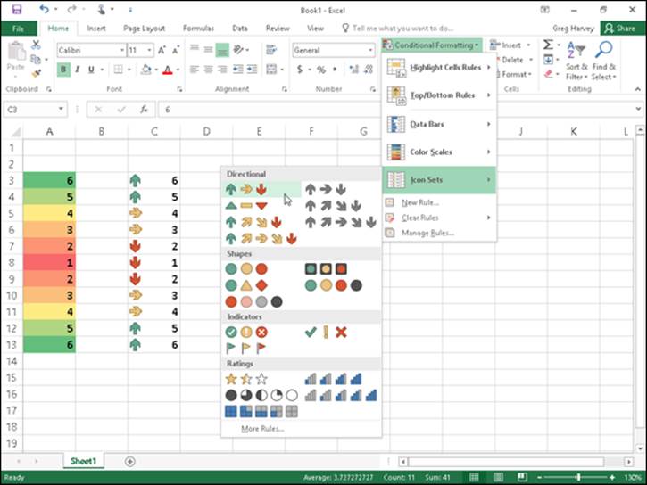
Figure 2-21: Conditionally formatting a sequence of numeric entries with the initial color scales and directional icons that graphically indicate their relative values.

If you want to hide the values in a cell range and only display a type of graphical conditional formatting, apply the desired graphical conditional formatting to the range of numeric entries and then hide the underlying values by formatting the same cell range with the custom numeric format that masks the numeric entries (;;;), as described in “Designing your own number formats,” earlier in this chapter.

Formatting with the Quick Analysis tool

Excel 2016’s Quick Analysis tool enables you to apply various types of conditional formatting to selected cell ranges. Figure 2-22 illustrates how this works. For this figure, I selected the cell range E3:E13 containing a copy of the range of values from 6 to 1 and 1 to 6 before clicking the Quick Analysis tool that routinely appears in the lower-right below the last selected cell.

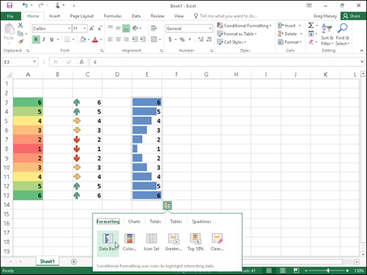
Figure 2-22: Using the Formatting tab’s options on the Quick Analysis tool’s palette to preview conditional formatting applied to a cell selection.

As soon as you select the Quick Analysis tool, the Formatting tab is automatically selected with its conditional formatting option buttons (Data Bars, Color Scale, Icon Set, Greater Than, Top 10%, and Clear Format) displayed. You can then use Live Preview to sample how the selected data would appear in different conditional formats. When you see one you like, you can then apply it by clicking the particular conditional formatting option button.

Identifying particular values or text entries in a cell range

The options attached to the Highlight Cell Rules and Top/Bottom Rules items on the Conditional Formatting button’s drop-down menu enable you to specify a particular type of formatting when certain conditions are met.

The rules that you set up for meeting these formatting conditions can vary widely. You can set up a rule whereby a particular type of formatting is applied when a cell in the range contains a certain text entry (such as Fixed or Variable). You set up a rule whereby a particular type of formatting is applied when a cell in the range is exactly a particular value or exceeds or falls below a particular value. So too, you can set up a rule whereby a particular type of formatting is applied when the value is one of the top ten in the range, is below the average value in the range, or falls into the lower ten percent.

For example, to set up the rule that Excel formats any cell within a range with a light red fill color and dark red font color whenever it contains the word Fixed, you follow these steps:

1. Select the range of cells in the worksheet to which this conditional formatting rule is to be applied.

2. Click the Conditional Formatting button on the Ribbon’s Home tab and then choose Highlight Cell Rules  ⇒  Text That Contains from the drop-down menu.

Excel opens the Text That Contains dialog box with a text box on the left where you enter or select in the worksheet the text that tells Excel when to apply the conditional formatting and a drop-down list box on the right where you select or define the conditional formatting the program is to apply.

3. Type Fixed in the Format Cells That Contain the Text box.

In this case, you don’t have to change the formatting in the drop-down list box, as Light Red Fill with Dark Red Text is the default formatting.

4. Click OK to apply the conditional formatting rule to the selected cell range.

Say you wanted to apply three different types of conditional formatting to the cells in a single range of the worksheet: one type of formatting whenever a cell in the range contains a target value, another when it exceeds this target value, and third when it falls below the target value.

Here are the steps for setting up the rules to apply a yellow fill with a dark yellow font to cells in a range when they contain 100,000, a green fill with dark green text when they’re greater than 100,000, and a light red fill with dark red text when they’re less than 100,000:

1. Select the range of cells in the worksheet to which the three conditional formatting rules are to be applied.

Start by defining the rule that applies yellow fill with dark yellow font to all values in the range that are equal to 100,000.

2. Click the Conditional Formatting button on the Home tab and then choose Highlight Cell Rules  ⇒  Equal To from the drop-down menu.

Excel opens the Equal To dialog box, where you define the formatting rule when a cell contains 100,000.

3. Type 100,000 in the Format Cells That Are EQUAL TO text box and then select Yellow Fill with Dark Yellow Text from the drop-down list box to the right before you click OK.

Next, you define the rule that applies green fill with dark green font to all values that are greater than 100,000.

4. Click the Conditional Formatting button on the Home tab and then choose Highlight Cell Rules  ⇒  Greater Than from the drop-down menu.

Excel opens the Greater Than dialog box, where you define the formatting rule when a cell contains a value higher than 100,000.

5. Type 100,000 in the Format Cells That Are GREATER THAN text box and then click Green Fill with Dark Green Text in the drop-down list box to the right before you click OK.

Finally, you define the rule that applies red fill with dark red font to all values that are less than 100,000.

6. Click the Conditional Formatting button on the Home tab and then choose Highlight Cell Rules  ⇒  Less Than from the drop-down menu

Excel opens the Less Than dialog box, where you define the formatting rule when a cell contains a value below 100,000.

7. Type 100,000 in the Format Cells That Are LESS THAN text box and then leave the default Light Red Fill with Dark Red Text selected in the drop-down list box to the right when you click OK.

As you define the three rules, Excel applies them to the range selected in the worksheet. If the cell range is blank at the time you set up these three rules, all the blank cells in the range are given a red fill. As you enter values into the cells, their text takes on the color assigned to their values: dark red font for values below 100,000, dark yellow for all values of 100,000, and dark green for all values above 100,000. In addition, when the values are equal to 100,000, Excel fills the cell with a light yellow background color and when values are above 100,000, a light green background color.

Finally, here are the steps you’d follow to create a rule that formats all values in a cell range that are below the average value in the range with a custom conditional format that applies bold italic to the font and a bright yellow fill color:

1. Select the range of cells in the worksheet to which this conditional formatting rule is to be applied.

2. Click the Conditional Formatting button on the Home tab and then choose Top/Bottom Rules  ⇒  Below Average from the drop-down menu.

Excel opens the Below Average dialog box that contains a single drop-down list box where you define the formatting to be used when a value is below the calculated average for the cell range.

3. Select Custom Format at the bottom of the Format Cells That Are BELOW AVERAGE drop-down list box.

Excel opens the Format Cells dialog box where you define all the attributes to be part of the custom conditional formatting.

4. Click the Font tab in the Format Cells dialog box and then click Bold Italic in the Font Style list box.

5. Click the Fill tab in the Format Cells dialog box and then click the bright yellow swatch in the Background Color section before you click OK.

Excel closes the Format Cells dialog box, returning you to the Below Average dialog box, which now displays Custom Format in the Format Cells That Are BELOW AVERAGE drop-down list box.

6. Click OK to close the Below Average dialog box.

Excel then applies the custom formatting of bold italic text with bright yellow fill color to all values in the cell selection that are below the calculated average (displayed after the Average heading on the status bar at the bottom of the Excel program window).

Highlighting duplicate values in a cell range

The Duplicate Values option on the Highlight Cell Rules continuation menu enables you to highlight duplicate values within a selected cell range.

To highlight duplicate values in a cell range, follow these steps:

1. Select the range of cells in the worksheet where you want duplicates formatted in a special way.

2. Click the Conditional Formatting button in the Styles group of the Home tab of the Ribbon; then choose Highlight Cell Rules  ⇒  Duplicate Values from the drop-down menu.

Excel opens the Duplicate Values Columns dialog box containing two drop-down lists: the first where you indicate whether Excel is to format identical values (Duplicate, the default) in the range or the standalone values (Unique) in the range, and the second where you indicate the type of formatting applied to either the duplicates or one-of-a-kind values.

3. Click the type of preset formatting (Red Fill with Dark Red Text, Yellow Fill with Dark Yellow Text, Green Fill with Dark Green Text, and so forth) or click the Custom Format option and select the custom formatting in the Format Cells dialog box.

If you define a custom format rather than select one of the preset formats, use the options on the Number, Font, Border, and Fill tabs of the Format Cells dialog box to designate all the formatting to be applied, and then click OK to close the Format Cells dialog box and return to the Compare Columns dialog box (where Custom Format appears in the third drop-down list box).

4. Click OK to close the Duplicate Values dialog box.

Excel then formats all the cells in the selected cell range whose values are exact duplicates with the conditional formatting you selected.

Creating your own conditional formatting rules

Although Excel 2016 gives you a ton of ready-made Highlight Cell Rules and Top/Bottom Rules to define, you may still find that you need to create your own rules for conditional formatting. To do this, you choose the New Rule option near the bottom of the Conditional Formatting button’s drop-down menu or you click the New Rule button in the Conditional Formatting Rules Manager dialog box. (See the “Managing conditional formatting rules” section that immediately follows.)

Figure 2-23 shows you the New Formatting Rule dialog box as it first appears after clicking the New Rule option or button. To create a new conditional formatting rule, you first click the type of rule to create in the Select a Rule Type list box and then specify the criteria and define the formatting using the various options that appear in the Edit the Rule Description section below — note that these options vary greatly depending on the type of rule you click in the Select a Rule Type list box above.

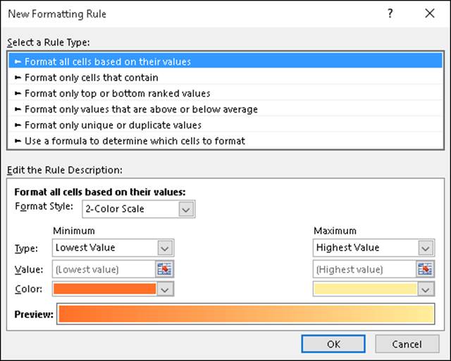
Figure 2-23: Define a new conditional formatting rule using the options in the New Formatting Rule dialog box.

Select the Use a Formula to Determine Which Cells to Format rule type when you want to build a formula as the rule that determines when a particular type of conditional formatting is applied. Note that this formula can refer to cells outside the current cell selection to which the conditional formatting is applied, but it must be a logical formula, meaning that it uses comparison operators (see Book III, Chapter 1) and/or Logical functions (see Book III, Chapter 2) that when calculated return either a logical TRUE or FALSE value.

Managing conditional formatting rules

The Conditional Formatting Rules Manager dialog box, which you open by choosing the Manage Rules option at the very bottom of the Conditional Formatting button’s drop-down menu, enables you to do all of the following:

· Create new rules by clicking the New Rule button to open the New Formatting Rule dialog box. (See the “Creating your own conditional formatting rules” section immediately preceding.)

· Edit existing rules by selecting the rule in the Rule list box and clicking the Edit Rule button in the Editing Formatting Rule dialog box (which looks just like the New Formatting Rule dialog box except it contains the rule type, criteria, and formatting for the particular rule you selected).

· Delete rules by clicking the rule in the Rule list box and then clicking the Delete Rule button — click the Apply button to remove formatting from the worksheet that was applied to the rule you just deleted.

· Change the order of precedence in which multiple conditional formatting rules assigned to the same cell selection or table are applied by promoting or demoting individual rules in the Rule list box by clicking the rules and then clicking either the Move Up button (with the thick arrow pointing upward) or Move Down button (with the thick arrow pointing downward) until the rules appear in the desired order of precedence.

By default, the Conditional Formatting Rules Manager dialog box shows all the rules assigned only to the current cell selection or table. To see all the conditional formatting rules in a particular worksheet or table, select its name from the Show Formatting Rules For drop-down list at the top of the dialog box.

A rule that appears higher in the Rule list box of the Conditional Formatting Rules Manager dialog box has a higher precedence and is therefore applied before one lower in the list. When more than one rule is true, what happens depends on whether or not the formatting applied by those rules conflict. When they don’t conflict (as when one rule formats the cells in bold italic and the other formats the cells with a light red fill), both formats are applied. However, when the formats conflict (as when one rule formats the cells with black fill and bright yellow text and the other formats the cells with yellow fill and black text), the rule with the higher precedence wins, and only its conditional formatting is applied.