Microsoft Excel 2016 BIBLE (2016)

IN THIS CHAPTER

1. Getting an overview of custom number formatting

2. Creating a custom number format

3. Listing all custom number format codes

4. Looking at examples of custom number formats

When you enter a number into a cell, you can display that number in a variety of different formats. Excel has quite a few built-in number formats, but sometimes none of them is exactly what you need.

This chapter describes how to create custom number formats and provides many examples that you can use as is or adapt to your needs.

About Number Formatting

By default, all cells use the General number format. This format is basically “what you type is what you get.” But if the cell isn't wide enough to show the entire number, the General format rounds numbers with decimals and uses scientific notation for large numbers. In many cases, the General number format works just fine, but most people prefer to specify a different number format for consistency.

The key thing to remember about number formatting is that it affects only how a value is displayed. The actual number remains intact, and any formulas that use a formatted number use the actual number.

Note

An exception to this rule occurs if you specify the Set Precision as Displayed option on the Advanced tab in the Excel Options dialog box. If that option is in effect, formulas use the values that are actually displayed in the cells as the result of a number format applied to the cells. In general, using this option is not a good idea because it changes the underlying values in your worksheet.

One more thing to keep in mind: if you use the Find and Replace dialog box (Home Editing Find & Select Find), characters that are displayed as a result of number formatting (for example, a currency symbol) are not searchable by default. To be able to locate information based on formatting, use the Look In Values option in the Find and Replace dialog box. If the Look In Values option is not visible, click the Options button to expand the dialog box.

Automatic number formatting

Excel is smart enough to perform some formatting for you automatically. For example, if you enter 12.3% into a cell, Excel assumes that you want to use a percentage format and applies it automatically. If you use commas to separate thousands (such as 123,456), Excel applies comma formatting for you. And if you precede your value with a currency symbol, Excel formats the cell for currency.

Note

You have an option when it comes to entering values into cells formatted as percentages. Access the Excel Options dialog box and click the Advanced tab. If the Enable Automatic Percent Entry check box is selected (the default setting), you can simply enter a normal value into a cell that has been formatted to display as a percent. (For example, enter 12.5 for 12.5%.) If this check box isn't selected, you must enter the value as a decimal (for example, .125 for 12.5%).

Excel automatically applies a built-in number format to a cell based on the following criteria:

· If a number contains a slash (/), it may be converted to a date format or a fraction format.

· If a number contains a hyphen (-), it may be converted to a date format.

· If a number contains a colon (:) or is followed by a space and the letter A or P (uppercase or lowercase), it may be converted to a time format.

· If a number contains the letter E (uppercase or lowercase), it may be converted to scientific notation (also known as exponential format). If the number doesn't fit into the column width, it may also be converted to this format.

Tip

At times, automatic number formatting can be frustrating. For example, if you enter a part number 10-12 into a cell, Excel converts it to a date. To avoid automatic number formatting when you enter a value, preformat the data input range with the desired number format or format the cell as text. Another option is to precede your entry with an apostrophe. The apostrophe makes the entry text, so number formatting is not applied to the cell.

Formatting numbers by using the Ribbon

The Number group on the Home tab of the Ribbon contains several controls for applying common number formats quickly. The Number Format drop-down control gives you quick access to 11 common number formats. In addition, the Number group contains some buttons. When you click one of these buttons, the selected cells take on the specified number format. Table 25.1 summarizes the formats that these buttons perform in the U.S. English version of Excel.

Table 25.1 Number-Formatting Buttons on the Ribbon

Note

Some of these buttons actually apply predefined styles to the selected cells. Access Excel's styles by using the Style gallery, in the Styles group on the Home tab. You can modify the styles by right-clicking the style name and choosing Modify from the shortcut menu. See Chapter 6, “Worksheet Formatting,” for details.

Using shortcut keys to format numbers

Another way to apply number formatting is to use shortcut keys. Table 25.2 summarizes the shortcut key combinations that you can use to apply common number formatting to the selected cells or range. Notice that these are the shifted versions of the number keys along the top of a typical keyboard.

Table 25.2 Number-Formatting Keyboard Shortcuts

Using the Format Cells dialog box to format numbers

For maximum control of number formatting, use the Number tab in the Format Cells dialog box. You can access this dialog box in any of several ways:

· Click the dialog box launcher at the bottom right of the Home Number group.

· Choose Home Number Number Format More Number Formats.

· Press Ctrl+1.

The Number tab in the Format Cells dialog box contains 12 categories of number formats from which to choose. When you select a category from the list box, the right side of the dialog box changes to display appropriate options.

Here are the number format categories, along with some general comments:

· General: The default format; it displays numbers as integers, as decimals, or in scientific notation if the value is too wide to fit into the cell.

· Number: Specify the number of decimal places, whether to use your system thousands separator (for example, a comma) to separate thousands, and how to display negative numbers.

· Currency: Specify the number of decimal places, choose a currency symbol, and display negative numbers. This format always uses the system thousands separator symbol (for example, a comma) to separate thousands.

· Accounting: Differs from the Currency format in that the currency symbols always line up vertically, regardless of the number of digits displayed in the value.

· Date: Choose from a variety of date formats and select the locale for your date formats.

· Time: Choose from a number of time formats and select the locale for your time formats.

· Percentage: Choose the number of decimal places; always displays a percent sign.

· Fraction: Choose from among nine fraction formats.

· Scientific: Displays numbers in exponential notation (with an E): 2.00E+05 = 200,000. You can choose the number of decimal places to display to the left of E.

· Text: When applied to a value, causes Excel to treat the value as text (even if it looks like a value). This feature is useful for such items as numerical part numbers and credit card numbers.

· Special: Contains additional number formats. The list varies, depending on the locale you choose. For the English (United States) locale, the formatting options are Zip Code, Zip Code +4, Phone Number, and Social Security Number.

· Custom: Define custom number formats not included in any of the other categories.

Note

If the cell displays a series of hash marks after you apply a number format (such as #########), it usually means that the column isn't wide enough to display the value by using the number format that you selected. Either make the column wider (by dragging the right border of the column header) or change the number format. A series of hash marks also can mean that the cell contains an invalid date or time.

Creating a Custom Number Format

When you create a custom number format, it can be used to format any cells in the workbook. You can create about 200 custom number formats in each workbook.

Figure 25.1 shows the Custom category in the Number tab of the Format Cells dialog box. Here, you can create number formats not included in any of the other categories. Excel gives you a great deal of flexibility in creating custom number formats.

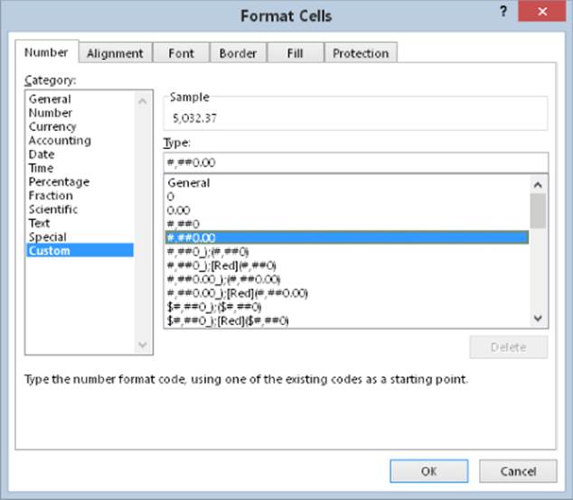
Figure 25.1 The Custom category of the Number tab in the Format Cells dialog box.

Tip

Custom number formats are stored with the workbook in which they are defined. To make the custom format available in a different workbook, you can just copy a cell that uses the custom format to the other workbook.

You construct a number format by specifying a series of codes as a number format string. You enter this code sequence in the Type field after you select the Custom category on the Number tab of the Format Cells dialog box. Here's an example of a simple number format code:

0.000

This code consists of placeholders and a decimal point; it tells Excel to display the value with three digits to the right of the decimal place. Here's another example:

00000

This custom number format has five placeholders and displays the value with five digits (no decimal point). This format is good to use when the cell holds a five-digit zip code. (In fact, this is the code actually used by the Zip Code format in the Special category.) When you format the cell with this number format and then enter a ZIP code, such as 06604, the value is displayed with the leading zero. If you enter this number into a cell with the General number format, it displays 6604 (no leading zero).

Scroll through the list of number formats in the Custom category in the Format Cells dialog box to see many more examples. In many cases, you can use one of these codes as a starting point, and you'll need to customize it only slightly.

The website for this book at www.wiley.com/go/excel2016bible contains a workbook with many custom number format examples (see Figure 25.2). The file is named number formats.xlsx.

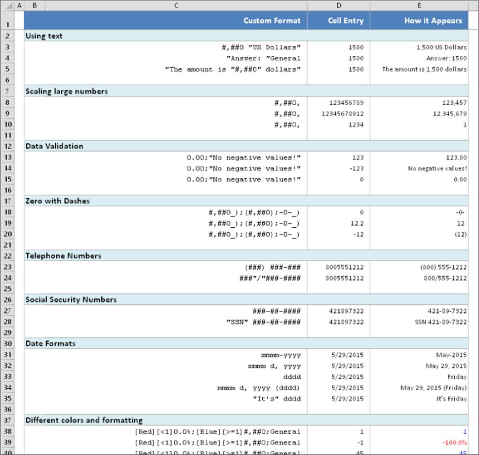
Figure 25.2 Examples of custom number formatting.

Parts of a number format string

A custom format string can have up to four sections, which enables you to specify different format codes for positive numbers, negative numbers, zero values, and text. You do so by separating the codes with a semicolon. The codes are arranged in the following order:

Positive format; Negative format; Zero format; Text format

If you don't use all four sections of a format string, Excel interprets the format string as follows:

· If you use only one section: The format string applies to all numeric types of entries.

· If you use two sections: The first section applies to positive values and zeros, and the second section applies to negative values.

· If you use three sections: The first section applies to positive values, the second section applies to negative values, and the third section applies to zeros.

· If you use all four sections: The last section applies to text stored in the cell.

The following is an example of a custom number format that specifies a different format for each of these types:

[Green]General;[Red]General;[Black]General;[Blue]General

This custom number format example takes advantage of the fact that colors have special codes. A cell formatted with this custom number format displays its contents in a different color, depending on the value. When a cell is formatted with this custom number format, a positive number is green, a negative number is red, a zero is black, and text is blue.

If you want to apply cell formatting automatically (such as text or background color) based on the cell's contents, a much better solution is to use the Excel Conditional Formatting feature. Chapter 21, “Visualizing Data Using Conditional Formatting,” covers conditional formatting.

Changing the Default Number Format for a Workbook

As I mentioned earlier, the default number format is General. If you prefer a different default number format, you have two choices: preformat the cells with the number format of your choice, or change the number format for the Normal style.

You can preformat specific cells, entire rows or columns, or even the entire worksheet. Just select the range and use any of the techniques described in this chapter to apply a number format to the selected cells.

Instead of preformatting an entire worksheet, however, a better solution is to change the number format for the Normal style. Unless you specify otherwise, all cells use the Normal style. Therefore, by changing the number format for the Normal style, you're essentially creating a new default number format for the workbook. The modified style applies to all new worksheets that you insert into the workbook.

Change the Normal style by displaying the Style gallery. Right-click the Normal style icon (in the Home Styles group) and choose Modify to display the Style dialog box. In the Style dialog box, click the Format button and then choose the new number format that you want to use for the Normal style.

Custom number format codes

Table 25.3 lists the formatting codes available for custom formats, along with brief descriptions. I use most of these codes in examples later in this chapter.

Table 25.3 Codes Used to Create Custom Number Formats

Table 25.4 lists the codes used to create custom formats for dates and times.

Table 25.4 Codes Used in Creating Custom Formats for Dates and Times

Where Did Those Number Formats Come From?

Excel may create custom number formats without your realizing it. When you use the Increase Decimal or Decrease Decimal button on the Home Number group of the Ribbon (or on the Mini toolbar), Excel creates new custom number formats, which appear on the Number tab in the Format Cells dialog box. For example, if you click the Increase Decimal button five times, the following custom number formats are created:

0.0

0.000

0.0000

0.000000

A format string for two decimal places is not created because that format string is built in.

Custom Number Format Examples

The remainder of this chapter consists of useful examples of custom number formats. You can use most of these format codes as is. Others may require slight modification to meet your needs.

Scaling values

You can use a custom number format to scale a number. For example, if you work with large numbers, you may want to display the numbers in thousands (that is, display 1,200,000 as 1,200). The actual number, of course, will be used in calculations that involve that cell. The formatting affects only the way it is displayed.

Displaying values in thousands

The following format string displays values without the last three digits to the left of the decimal place and no decimal places. In other words, the value appears as if it's divided by 1,000 and rounded to no decimal places.

#,###,

A variation of this format string follows. A value with this number format appears as if it's divided by 1,000 and rounded to two decimal places.

#,###.00,

Table 25.5 shows examples of these number formats.

Table 25.5 Examples of Displaying Values in Thousands

Displaying values in hundreds

The following format string displays values in hundreds, with two decimal places. A value with this number format appears as if it's divided by 100 and rounded to two decimal places.

0"."00

Table 25.6 shows examples of these number formats.

Table 25.6 Examples of Displaying Values in Hundreds

Displaying values in millions

The following format string displays values in millions with no decimal places. A value with this number appears as if it's divided by 1,000,000 and rounded to no decimal places:

#,###,,

A variation of this format string follows. A value with this number appears as if it's divided by 1,000,000 and rounded to two decimal places:

#,###.00,,

Here's another variation. This format string adds the letter M to the end of the value:

#,###,,M

The following format string is a bit more complex. It adds the letter M to the end of the value, displays negative values in parentheses, and displays zeros:

#,###.0,,"M"_);(#,###.0,,"M)";0.0"M"_)

Table 25.7 shows examples of these format strings.

Table 25.7 Examples of Displaying Values in Millions

Appending zeros to a value

The following format string displays a value with three additional zeros and no decimal places. A value with this number format appears as if it's rounded to no decimal places and then multiplied by 1,000:

#",000"

Examples of this format string, plus a variation that adds six zeros, are shown in Table 25.8.

Table 25.8 Examples of Displaying a Value with Extra Zeros

Displaying leading zeros

To display leading zeros, create a custom number format that uses the 0 character. For example, if you want all numbers to display with ten digits, use the number format string that follows. Values with fewer than ten digits will display with leading zeros:

0000000000

You can force all numbers to display with a fixed number of leading zeros. The format string that follows, for example, appends three zeros to the beginning of each number:

"000"#

Specifying conditions

The following custom number format displays text, based on the value of the cell:

[<10]"Too low";[>10]"Too high";"Just right"

If the value is less than 10, it displays Too low. If the value is greater than 10, it displays Too high. If the value is exactly 10, it displays Just right. Note that you can specify only one or two conditions, plus an “other.”

Generally, using Excel's conditional formatting feature is a better solution for formatting that's based on a value. See Chapter 21 for details.

Displaying fractions

Excel supports quite a few built-in fraction number formats. (Select the Fraction category on the Number tab in the Format Cells dialog box.) For example, to display the value .125 as a fraction with 8 as the denominator, select As Eighths (4/8) from the Type list (see Figure 25.3).

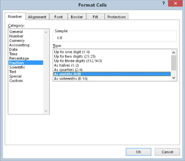
Figure 25.3 Selecting a number format to display a value as a fraction.

You can use a custom format string to create other fractional formats. For example, the following format string displays a value in 50ths:

# ??/50

To display the fraction reduced to its lowest terms, use a question mark after the slash symbol. For example, the value 0.125 can be expressed as 2/16, and 2/16 can be reduced to 1/8. Here's an example of a number format that displays the value as a fraction reduced to its simplest terms:

# ?/?

If you omit the leading hash mark, the value is displayed without a leading value. For example, the value 2.5 would display as 5/2 using this number format code:

?/?

The following format string displays a value in terms of fractional dollars. For example, the value 154.87 is displayed as 154 and 87/100 Dollars:

0 "and "??/100 "Dollars"

The following example displays the value in sixteenths, with a quotation mark appended to the right. This format string is useful when you deal with fractions of inches (for example, 2/16”).

# ??/16\"

Displaying a negative sign on the right

The following format string displays negative values with the negative sign to the right of the number. Positive values have an additional space on the right, so both positive and negative numbers align properly on the right:

#,##0.00_-;#,##0.00-

To make the negative numbers more prominent, you can add a color code to the negative part of the number format string:

#,##0.00_-;[Red]#,##0.00-

Formatting dates and times

When you enter a date into a cell, Excel formats the date using the system short date format. You can change this format by using the Windows Control Panel (Regional and Language Options).

Excel provides many useful, built-in date and time formats. Table 25.9 shows some other date and time formats that you may find useful. The first column of the table shows the date/time serial number.

Table 25.9 Useful Built-In Date and Time Formats

See Chapter 12, “Working with Dates and Times,” for more information about the Excel date and time serial number system.

Displaying text with numbers

The ability to display text with a value is sometimes useful. To add text, just create the number format string as usual (or use a built-in number format as a starting point) and put the text within quotation marks. The following number format string, for example, displays a value with the text (US Dollars) added to the end:

#,##0.00 "(US Dollars)"

Here's another example that displays text before the number:

"Average: "0.00

If you use the preceding number format, you'll find that the negative sign appears before the text for negative values. To display number signs properly, use this variation:

"Average: "0.00;"Average: "-0.00

The following format string displays a value with the words Dollars and Cents. For example, the number 123.45 displays as 123 Dollars and .45 Cents. Technically, the decimal point should not appear in the amount before Cents, but there's no way to eliminate it:

0 "Dollars and" .00 "Cents"

Testing Custom Number Formats

The TEXT function displays a number using a number format string specified as the second argument. The TEXT function uses the same number formatting codes as standard number formatting. Use this to your advantage when creating a custom number format.

The figure shows a worksheet with four entries in column A: a positive value, zero, a negative value, and text. Cell B1 contains a custom formatting string. Cell C1 contains this formula, which was copied to the three cells below:

=TEXT(A1,$B$1)

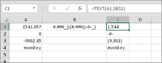
When you modify the number formatting string in cell B1, the cells in column C update.

This technique works well, and editing a number format string in a cell is much easier than doing it directly in the Format Cells dialog box. However, the technique has some limitations:

· The TEXT function does not handle color codes.

· The TEXT function does not handle the asterisk code (used to repeat text)

· Codes in the text string are not translated if you open the workbook in a different language version of Excel.

When you're satisfied, just copy the text in B1 and paste it into the Format Cells dialog box. Then you can apply this custom format for any cells.

Suppressing certain types of entries

You can use number formatting to hide certain types of entries. For example, the following format string displays text but not values:

;;

This format string displays values but not text or zeros:

0.0;-0.0;;

This format string displays everything except zeros:

0.0;-0.0;;@

You can use the following format string to completely hide the contents of a cell:

;;;

Note that when the cell is activated, however, the cell's contents are visible on the Formula bar.

Filling a cell with a repeating character

The asterisk (*) symbol specifies a repeating character in a number format string. The repeating character completely fills the cell and adjusts if the column width changes. The following format string, for example, displays the contents of a cell padded on the right with dashes:

General*-;-General*-;General*-;General*-