Expert Cube Development with SSAS Multidimensional Models (2014)
Chapter 6. Adding Calculations to the Cube
This chapter explains how to enhance the analytical capabilities of our cube with MDX calculations. Calculations, especially calculated members, are very common in cubes as they are a very easy and convenient way to generate new and useful business metrics from the basic values you have imported from your data warehouse.
This chapter does not cover basic MDX concepts, although we will provide several examples of MDX usage. For a complete reference of the MDX language, or for a thorough tutorial, you should refer to other books, such as MDX Solutions, Fast Track to MDX,Microsoft SQL Server 2008 MDX Step by Step, or MDX with SSAS 2012 Cookbook.
Reading this chapter, you will learn about:
· The different kinds of calculated members
· Several ready-to-use examples of calculated members
· The difference between using calculated measures and calculation dimensions
· Defining and using named sets
Different kinds of calculated members
There are three kinds of calculated members:
· Query-scoped calculated members: These are calculated members defined in the WITH clause of an MDX query. They are specific to the query and cannot be referenced outside it. They are very useful to developers for testing, debugging, and ad hoc reporting, but as defining a calculated member requires knowledge of MDX, it is not something a normal end user will be able to do.
· Session-scoped calculated members: These are calculated members that exist in the context of the session created when a user connects to a cube. These calculated members are available for use in all queries executed in a particular session until either the session is closed or the calculated members are dropped. Session calculations are a convenient means for a client tool to simplify the queries it generates, but apart from that, they are rarely used. They are created by the client tool executing a CREATE MEMBER statement.
· Globally-scoped calculated members: These are calculated members defined in the MDX Script of the cube using CREATE MEMBER statements. They are available for use in queries to all users and can be used in the very same way as physical members are. They are the most common kind of calculated members.
At first glance, we might think that the only difference between these three ways to define a calculated member is how long they are available and to whom. However, as we will see in Chapter 8, Query Performance Tuning, the scope of a calculated member determines how long the values it returns can be cached, and this, in turn, can have a significant impact on query performance.
At this stage, though, all we need to understand is that globally-scoped calculated members are best from a performance point of view. Remember also that by defining a calculated member on the cube, we are removing the need for other developers (for example, Reporting Services report authors) to define these calculations in their own queries. If too many calculations end up being defined in queries rather than on the cube it can lead to duplication of effort, confusion when different calculations are given the same name in different queries, and maintenance problems. In fact, fixing a bug in a calculation involves tracking down multiple instances of the same calculation and, possibly, we end up having different calculations in different queries for the same formula. For all of these reasons, we recommend that you should always try to create calculated members on the cube, and only use session-scoped or query-scoped calculations when you have no other choice.
Common calculations
We are now going to show some very common types of calculated members. As stated before, the goal here is not to spend a lot of time explaining how the MDX code actually works, but to show some examples of calculations that can be copied and adapted easily for almost any cube.
Simple calculations
The simplest kind of calculated members are those that perform basic arithmetic on other measures. For example, we might have two real measures in the cube that represent our sales and our costs; to calculate our profit, we just need to subtract costs from sales.
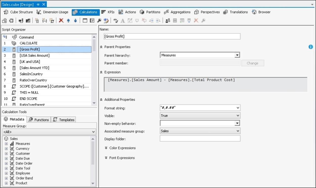
To add a calculation like this to the cube all we need to do is open the Cube Editor in SQL Server Data Tools (SSDT), go to the Calculations tab, and once we're there we have a choice of two options to create a calculated measure. By default, the Calculationstab opens in Form View, and to create a calculated member here we simply need to click on the New Calculated Member button and fill in all of the properties as required; behind the scenes SSDT will generate an MDX CREATE MEMBER statement for us that will create the calculated member.
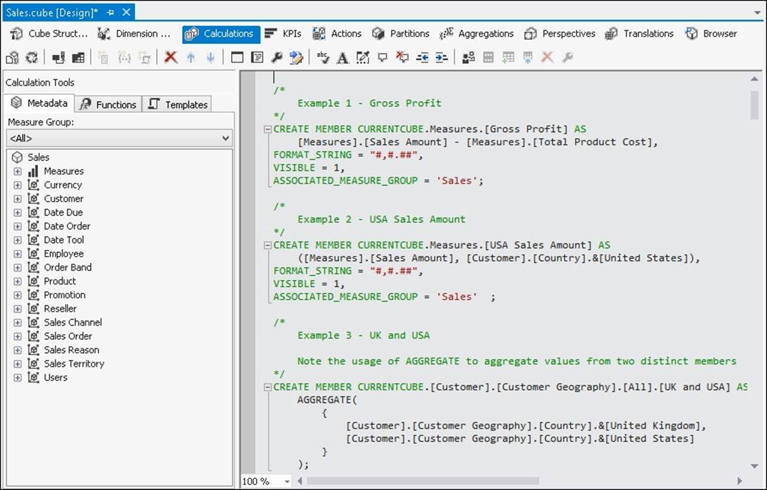
If we click on the Script View button on the toolbar, we are able to see what the MDX generated actually looks like, and we can also write our own code there if need be:
Here is an example of what the CREATE MEMBER statement for a Profit calculated measure looks like:
CREATE MEMBER CURRENTCUBE.Measures.[Gross Profit]
AS [Measures].[Sales Amount] - [Measures].[Total Product Cost],
FORMAT_STRING = "#,#.##",
VISIBLE = 1;
This statement creates a new member on the Measures dimension. As you can see, the expression used to do the calculation is very simple:
[Measures].[Sales Amount] - [Measures].[Total Product Cost]
One point to note here is that we refer to each real measure in the expression using its Unique Name: for example, the Sales Amount measure's unique name is [Measures].[Sales Amount]. A unique name is exactly what you'd expect, a way of uniquely identifying a member among all the members on all the hierarchies in the cube. You can write MDX without using unique names, just using member names instead:
[Sales Amount] - [Total Product Cost]
However, we strongly recommend you always use unique names even if it means your code ends up being much more verbose. This is because there may be situations where Analysis Services takes a long time to resolve a name to a unique name; and there is also the possibility that two members on different hierarchies will have the same name, in which case you won't know which one Analysis Services is going to use.
Referencing cell values
A slightly more complex requirement that is often encountered is to be able to reference not just another measure's value, but the value of another measure in combination with other members on other hierarchies. For example, you might want to create a calculated measure that always displays the sales for a particular country. Here's how you can do this:
CREATE MEMBER CURRENTCUBE.Measures.[USA Sales Amount]
AS
([Measures].[Sales Amount], [Customer].[Country].&[United States]),
FORMAT_STRING = "#,#.##",
VISIBLE = 1 ;
The expression we've used here in our calculated measure definition consists of a single tuple. In MDX, a tuple is a way of referencing the value of any cell in the cube; the definition of a tuple consists of a comma-delimited list of unique names of members from different hierarchies in the cube, surrounded by round brackets. In the preceding example, our tuple fixes the value of the calculated measure to that of the Sales Amount measure and the Customer Country United States.
The behavior of this new calculation can be easily seen when we browse the cube by Customer Country:
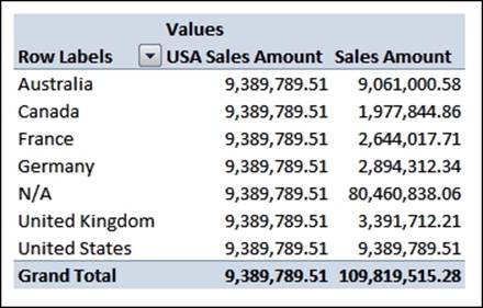
As you can see, while the Sales Amount measure always shows the sales for the country displayed on rows, the new calculated measure always shows sales for the USA. This is always the case no matter what other hierarchies are used in the query or where the measure itself is used:
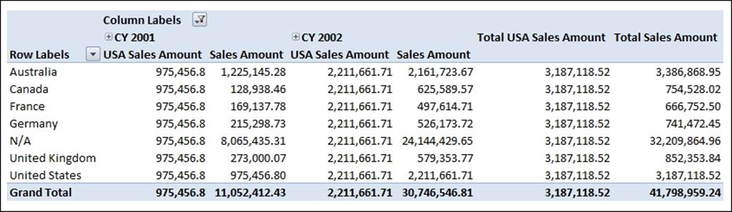
The calculated measure always shows the value of sales for the USA, even when we have broken sales down by Year. If we wanted to fix the value of the calculated measure by one more hierarchy, perhaps to show sales for male customers in the USA, we would just add another member to the list in the tuple as follows:
([Measures].[Sales Amount], [Customer].[Country].&[United States], [Customer].[Gender].&[Male])
Aggregating members
A tuple cannot, however, contain two members from the same hierarchy. If we need to do something like show the sum of sales in the UK and USA, we need to use the AGGREGATE functions on a set containing those two members:
CREATE MEMBER
CURRENTCUBE.[Customer].[Customer Geography].[All].[UK and USA] AS
AGGREGATE(
{[Customer].[Customer Geography].[Country].&[United Kingdom],
[Customer].[Customer Geography].[Country].&[United States]});
The preceding statement creates a new member on the Customer Geography hierarchy of the Customer dimension called UK and USA, and uses the AGGREGATE function to return their combined value.
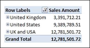
Year-to-date calculations
Year-to-date calculations calculate the aggregation of values from the 1st of January up to the current date. In order to create a year-to-date calculation, we need to use the YTD function, which takes a single date member as a parameter and returns the set of members on the same hierarchy as that member starting from the first day of the year up to and including the selected member. So, for example, if we passed the member 23rd July into the YTD function, we'd get a set containing all of the dates from 1st January to 23rd July; it also works at higher levels, so if we passed in the member Quarter 3, we'd get a set containing Quarter 1, Quarter 2, and Quarter 3.
In order for the YTD function to work properly, you need to have a dimension whose Type property is set to Time, an attribute hierarchy in that dimension whose Type property is set to Years, and a user hierarchy including that attribute hierarchy (see the sectionConfiguring a Time dimension in Chapter 2, Building Basic Dimensions and Cubes, for more details on the Type property). This is because the way the function works is to take the member you pass into it, find its ancestor at the Year level, find the first member of that year on the same level as the original member we passed in, and then return the set of all members between the first member in the year and the member we passed in.
Passing a static member reference into the YTD function is not going to be very useful – what we want is to be able to make it dynamic and return the correct year-to-date set for all of the dates we use in our queries. To do this, we can use the CurrentMember function on our date hierarchy, and use it to pass a reference to the current date member from the context of our query into our calculated member.
Finally, the YTD function only returns a set object, and what we need to do is to return the sum of that set for a given measure. As a result, our first attempt at writing the calculated member, building on what we saw in the previous section, might be something like this:
CREATE MEMBER CURRENTCUBE.Measures.[Sales Amount YTD] AS
SUM (
YTD ([Date Order].[Calendar].CurrentMember),
Measures.[Sales Amount]);
This computes the Sales Amount YTD member as the sum of the sales amount from the first date in the year up to and including the currently selected member in the date order calendar hierarchy.
The formula is correct in this case, but in order to make it work properly for any measure, we should use the following:
CREATE MEMBER CURRENTCUBE.Measures.[Sales Amount YTD] AS
AGGREGATE (
YTD ([Date Order].[Calendar].CurrentMember),
Measures.[Sales Amount]);
Here we replaced the MDX SUM function with AGGREGATE. The result for Sales Amount is the same. However, if we need to use this formula on a measure that does not have its AggegationFunction property set to Sum, AGGREGATE will aggregate values differently for each different AggegationFunction, whereas SUM will always provide the sum. For example, consider a measure that has its AggegationFunction property set to DistinctCount: if we had 5 distinct customers on 1st January, 3 distinct customers on 2nd January, and 4 distinct customers on 3rd January, the total number of distinct customers from the 1st to the 3rd of January would not be 5+3+4=12 because some customers might have sales on more than one day. Using AGGREGATE in this case will provide the correct number of distinct customers in the year-to-date.
Ratios over a hierarchy
Another very common pattern of calculated member is the ratio. A good example of this is when we want to compute the ratio of a measure (for example, sales amount) on a member of a hierarchy against its parent.
Consider, for example, the Customer Geography hierarchy in the Customer dimension. We might want to compute two different kinds of ratios:
· Ratio over Country: This is the ratio of the selected member against the whole of the country. This gives a percentage that shows how much a State or City's sales contribute to the sales of the whole country.
· Ratio over Parent: This is the ratio of the selected member against its parent in the hierarchy rather than the whole country. So, for example, we would see the percentage contribution of a City to the Region it was in, if City was the level immediately underneath Region in the hierarchy.
The difference between the two ratios is evident in the following screenshot:
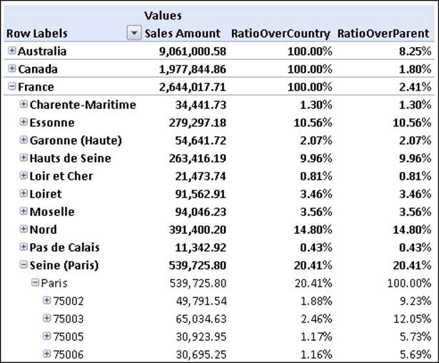
We can easily see that the RatioOverCountry of the ZIP code 75002 in Paris is 1.88% while the RatioOverParent is 9.23%. The difference is in the denominator in the formula: in the RatioOverCountry the denominator is the total of France while in the RatioOverParent the denominator is the total of Paris.
The RatioOverCountry measure is slightly easier to define because the denominator is clearly defined as the Country defined by the selection. The MDX code is pretty simple:
CREATE MEMBER CURRENTCUBE.Measures.RatioOverCountry AS
([Measures].[Sales Amount]) /
(
[Measures].[Sales Amount],
Ancestor (
[Customer].[Customer Geography].CurrentMember,
[Customer].[Customer Geography].Country
)
),
FORMAT_STRING = "Percent";
As the numerator, we put the sales amount; in the denominator we override the Geography hierarchy with the ancestor of the CurrentMember at the level of Country. So, if this measure is evaluated for ZIP code 75002 of Paris, the following will happen: [Customer].[Customer Geography].CurrentMember evaluates to 75002, and its ancestor, at Country level, evaluates to France. In the numerator, the Customer Geography hierarchy evaluates to 75002, while at the denominator, we provide an explicit substitution and the same hierarchy evaluates to Paris. The ratio between those two values for the Sales Amount measure is the percentage required.
We use the format string Percent that transforms decimal numbers into percentages (0.1234 is 12.34 percent, 1 is 100 percent, and 2.5 is 250 percent).
The second version of the ratio is similar, and simply changes the denominator from the fixed ancestor at the Country level to a relative one. The denominator is relative to the CurrentMember: it is its parent. The formula is:
CREATE MEMBER CURRENTCUBE.Measures.RatioOverParent AS
(Measures.[Sales Amount])
/
(
Measures.[Sales Amount],
Customer.[Customer Geography].CurrentMember.Parent
),
FORMAT_STRING = "Percent";
The numerator is the same measure, but the denominator changes each time the CurrentMember changes and is expressed as the parent of the CurrentMember. The Parent function returns the immediate ancestor of a member in its hierarchy. So, when the CurrentMemberevaluates to ZIP code 75002 its parent will be Paris. When the CurrentMember is Paris its parent will be Seine (Paris) and so on.
If we query the cube with these two formulas, we will get this result:
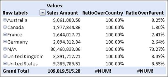
We can easily check that the value is correctly computed, but at the Grand Total level, we get two errors. The reason for this is that the Customer Geography hierarchy is at the All level and so the denominator in the formula has no value because:
· There is no ancestor of the CurrentMember at the country level, as it is already at the top level, so this causes the error in RatioOverCountry
· There is no parent at the top level in the hierarchy, so this causes the error in RatioOverParent
Since we know that the ratio has no meaning at all at the top level, we can use a SCOPE statement to overwrite the value at the top level with NULL.
SCOPE ([Customer].[Customer Geography].[All], Measures.RatioOverParent);
THIS = NULL;
END SCOPE;
SCOPE ([Customer].[Customer Geography].[All], Measures.RatioOverParent);
THIS = NULL;
END SCOPE;
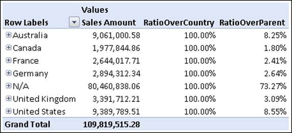
The two SCOPE statements will provide a better user experience, clearing values that should not be computed due to functional limitations on their meaning:
There is still a problem that should be addressed: what if the denominator evaluates to zero in some cases? The evaluation of any number divided by zero will show a value of infinity - which will look like an error to the user - and this is not a situation we would like to happen. For this reason, it is always a good practice to check for a zero denominator just before performing the division.
The function to use to make this check is IIF. It takes three parameters and if the first evaluates to True, it returns the value of the second parameter, otherwise it returns the third one. We can now rephrase the ratio as:
CREATE MEMBER CURRENTCUBE.Measures.RatioOverCountry AS
IIF (
(
[Measures].[Sales Amount],
Ancestor (
[Customer].[Customer Geography].CurrentMember,
[Customer].[Customer Geography].Country
)
) = 0,
NULL,
([Measures].[Sales Amount]) /
(
[Measures].[Sales Amount],
Ancestor (
[Customer].[Customer Geography].CurrentMember,
[Customer].[Customer Geography].Country
)
)
),
FORMAT_STRING = "Percent";
Note
You might be wondering: what happens if we try to divide by NULL instead of zero? In fact the same thing happens in both cases, but the preceding code traps division by NULL as well as division by zero because in MDX, the expression 0=NULL evaluates to true. This behavior can come as a bit of a shock, especially to those people with a background in SQL, but in MDX, it causes no practical problems and is actually quite helpful.
Even if this formula is correct, it still has two problems:
· It is not very easy to understand because of the repetition of the formula to get the sales at the Country level, first in the division-by-zero check and second in the ratio calculation itself.
· The value of the sales at the Country level will not be cached and so it will lead to a double computation of the same value. Analysis Services can only cache the value of an entire calculation, but can't cache the results of expressions used inside a calculation.
Luckily, one simple correction to the formula solves both problems, leading to a much clearer and optimized expression. We define a hidden member, SalesInCountry, that returns the sales in the current country and then substitute it for the expression returning sales at the Country level in the original calculation:
CREATE MEMBER CURRENTCUBE.Measures.SalesInCountry AS
(
[Measures].[Sales Amount],
Ancestor (
[Customer].[Customer Geography].CurrentMember,
[Customer].[Customer Geography].Country
)
),
VISIBLE = 0;
CREATE MEMBER CURRENTCUBE.Measures.RatioOverCountry AS
IIF (
Measures.SalesInCountry = 0,
NULL,
([Measures].[Sales Amount]) / Measures.SalesInCountry
),
FORMAT_STRING = "Percent";
The new intermediate measure has the property VISIBLE set to 0, which means that the user will not see it. Nevertheless, we can use it to make the next formula clearer and to let the formula engine cache its results in order to speed up computation.
With SSAS 2012 SP1, you can easily rewrite the previous code in a more elegant way by using the new DIVIDE function. DIVIDE makes it easier to write divisions without having to worry about the initial IIF to check the denominator for zero or NULL:
CREATE MEMBER CURRENTCUBE.Measures.RatioOverCountry AS
DIVIDE (
[Measures].[Sales Amount],
Measures.SalesInCountry,
NULL
),
FORMAT_STRING = "Percent";
The DIVIDE function accepts three parameters: numerator, denominator, and default value. In case the denominator evaluates to zero or NULL, DIVIDE returns the default value instead of raising an error.
It is worth to note that DIVIDE is useful to avoid the test for the division by zero, but it does not solve the issue of caching the intermediate result. The definition of the SalesInCountry measure is still useful, even if DIVIDE is used.
Previous period growths
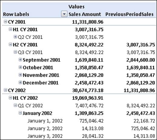
A previous period growth calculation is defined as the growth, either in percentage or absolute value, from the previous time period to the current one. It is very useful when used with a time hierarchy to display the growth of the current month, quarter or year over the previous month, quarter or year.
The key to solving this particular calculation is the PrevMember function, which returns the member immediately before any given member on a hierarchy. For example, if we used PrevMember with the Calendar Year 2003, it would return the Calendar Year 2002. As a first step, let's create a calculated member that returns Sales for the previous period to the current period, again using the Currentmember function to get a relative reference to the current time period:
CREATE MEMBER CURRENTCUBE.Measures.PreviousPeriodSales AS
(Measures.[Sales Amount],
[Date Order].[Calendar].CurrentMember.PrevMember),
FORMAT_STRING = "#,#.00";
Here, we take the CurrentMember on the Calendar hierarchy, and then use PrevMember to get the member before it. In order to get the sales figures for that time period, we've created a tuple, which is simply a comma-delimited list of members from different hierarchies in the cube enclosed in round brackets. You can think of a tuple as a coordinate to a particular cell within the cube; when we use a tuple in a calculation, it will always return the value from the cell it references.
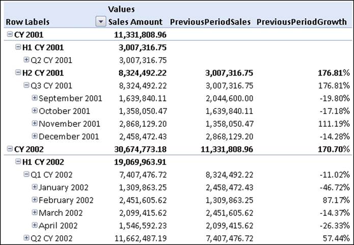
Having calculated the previous member sales, it is now very easy to compute the growth percentage, taking care to handle, as before, division by zero.
CREATE MEMBER CURRENTCUBE.Measures.PreviousPeriodGrowth AS
DIVIDE (,
Measures.[Sales Amount] - Measures.PreviousPeriodSales,
Measures.PreviousPeriodSales
),
FORMAT_STRING = "#,#.00%";
This produces the following output:
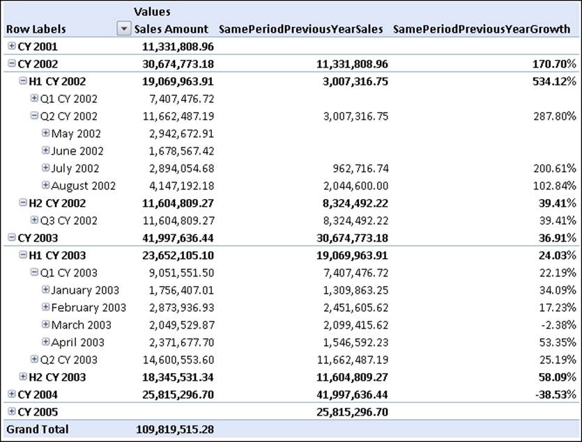
Same period previous year
In a similar way to the previous period calculation, we might want to check the sales of the current month against the same month in the previous year. The function to use here is ParallelPeriod, which takes three parameters: a level, the number of periods to go back, and a member. It takes the ancestor of the member at the specified level, goes back the number of periods specified at that level, and then finds the child of the member at the same level as the original member, in the same relative position as the original member was.
Here's an example of how it can be used in a calculated measure:
CREATE MEMBER CURRENTCUBE.Measures.SamePeriodPreviousYearSales AS
(Measures.[Sales Amount],
ParallelPeriod (
[Date Order].[Calendar].[Calendar Year],
1,
[Date Order].[Calendar].CurrentMember)),
FORMAT_STRING = "#,#.00";
Here we pass to ParallelPeriod the Year level, the fact we want to go back 1 period, and as a starting point, the current member of the Date Order dimension's Calendar hierarchy; the result is that ParallelPeriod returns the same period as the current member onCalendar but in the previous year.
Having calculated the sales in the same period in the previous year, it is straightforward to calculate the percentage growth. Note that here we are handling two different situations where we want to return a NULL value instead of a number: when there were no sales in the previous period (when it would otherwise show a useless 100%) and when there are no sales in the current period (when it would otherwise show a useless -100%).
CREATE MEMBER CURRENTCUBE.Measures.SamePeriodPreviousYearGrowth AS
IIF (
Measures.SamePeriodPreviousYearSales = 0,
NULL,
IIF (
Measures.[Sales Amount] = 0,
NULL,
(Measures.[Sales Amount] - Measures.SamePeriodPreviousYearSales) /
Measures.SamePeriodPreviousYearSales)),
FORMAT_STRING = "Percent";
The final result of this formula is shown here:
Moving averages
Moving averages are another very common and useful kind of calculation. While the calculations we've just seen compare the current period against a fixed point in the past, moving averages are useful in determining the trend over a time range, for example, showing the average sales of the last 12 months.
Depending on our requirements, we'll want to use different time ranges to calculate the average. This is because moving averages are generally used to show long-term trends by reducing seasonal, or random, variations in the data. For example, if we are looking at the sales of ice cream then sales in summer will be much greater than in winter, so we would want to look at an average over 12 months to account for seasonal variations. On the other hand, if we were looking at sales of something like bread where there was much less of a seasonal component, a three month moving average might be more useful.
The following formula we show for a moving average uses a function similar to the YTD function used before to compute Year-to-Date values, but is more flexible: LastPeriods. We can think of YTD as returning a time range that always starts at January 1st, while moving averages need a dynamic range that starts at a given number of periods before the current member. LastPeriods returns a range of time periods of a given size, ending with a given member, which is exactly what we need for our moving average calculation.
In some situations, the number of items in the moving window might be less than we specified. At the start of our time dimension, or before sales for a particular product have been recorded, the number of periods in our range will be smaller because if we use a six month window, we might not have data for a whole six months. It is important to decide what to show in these cases. In our example, we will show empty values since, having fewer months, we consider the average not meaningful.
Let us start with a basic version of the calculation that will work at the month level:
CREATE
MEMBER CURRENTCUBE.Measures.AvgSixMonths AS
IIF (
Count (
NonEmpty (
LastPeriods (6,
[Date Order].[Calendar].CurrentMember
),
Measures.[Sales Amount]
)
) <> 6,
NULL
Avg (
LastPeriods (6,
[Date Order].[Calendar].CurrentMember
),
Measures.[Sales Amount]
)
),
FORMAT_STRING = "#,#.00" ;
The first part of the calculation makes use of two functions, NonEmpty and LastPeriods, to check if the required six months are available to have a meaningful average.
· NonEmpty takes two sets and removes the tuples from the first set that are empty when evaluated across the tuples in the second set. Because our second parameter is a measure, we get only the tuples in the first set where the measure evaluates to a non NULLvalue.
· LastPeriods returns, as we've seen, the previous n members from its second parameter.
So, the calculation takes the set of the last six months then removes the ones where there are no sales and checks if the number of items left in the set is still six. If not, the set contains months without sales and the average will be meaningless, so it returns a NULL value. The last part of the formula computes the average over the same set computed before using the AVG function for Sales Amount.
This version of the calculation works fine for months, but at other levels of the Calendar hierarchy it doesn't – it's a six time period moving average, not a six month moving average. We might decide we want to use completely different logic at the Date or Quarter level; we might even decide that we don't want to display a value at anything other than the Month level. How can we achieve this?
We have two options: use scoped assignments, or add some more conditional logic in the calculation itself. In Analysis Services 2005, scoped assignments were the best choice for performance reasons, but in later releases of Analysis Services, the two approaches are more or less equivalent in this respect; and since adding conditional logic in the calculation itself is much easier to implement, we'll take that approach instead. What we need is another test that will tell us if the CurrentMember on Calendar is at the Month level or not. We can use the Level function to return the level of the CurrentMember; we then need to use the IS operator to compare what the Level function returns with the Month level as follows:
CREATE
MEMBER CURRENTCUBE.Measures.AvgSixMonths AS
IIF (
NOT
[Date Order].[Calendar].CurrentMember.Level
IS
[Date Order].[Calendar].[Month]OR
Count (
NonEmpty (
LastPeriods (6,
[Date Order].[Calendar].CurrentMember
),
Measures.[Sales Amount]
)
) <> 6,
NULL,
Avg (
LastPeriods (
6,
[Date Order].[Calendar].CurrentMember
),
Measures.[Sales Amount]
)
),
FORMAT_STRING = "#,#.00" ;
For more detail on implementing more complex moving averages, such as weighted moving averages, take a look at the following post on Mosha Pasumansky's blog: http://tinyurl.com/moshaavg.
Ranks
Often we'll want to create calculated measures that display rank values, for example, the rank of a product based on its sales. Analysis Services has a function for exactly this purpose: the Rank function, which returns the rank of a member inside a set. It's important to realize that the Rank function does not sort the set it uses, so we'll have to do that ourselves using the Order function as well.
Here's an example calculated measure that displays the rank of the current member on the Products hierarchy within all of the members on the same level, based on the Sales Amount measure:
CREATE
MEMBER CURRENTCUBE.Measures.ProductRank AS
IIF (
Measures.[Sales Amount] = 0,
NULL,
Rank (
Product.Products.CurrentMember,
Order (
Product.Products.CurrentMember.Level.MEMBERS,
Measures.[Sales Amount],
BDESC
)
)
);
As usual, we test to see if the Sales Amount measure is zero or empty; if it is, there's no point displaying a rank. Then, we take the set of all members on the same level of the current member of the Products hierarchy, order that set by Sales Amount in descending order, and return the rank of the CurrentMember inside that set.
Then, we can use the calculated member in reports like this:
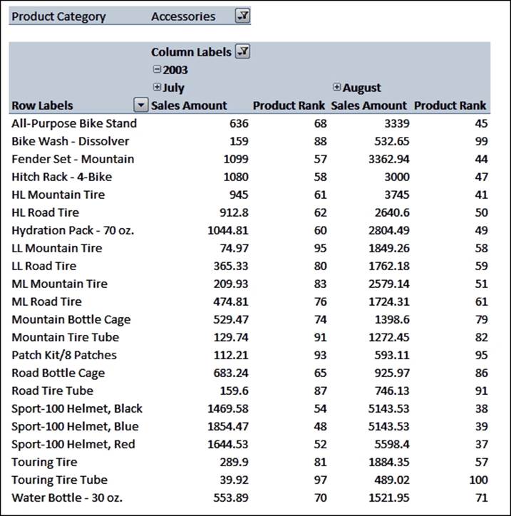
You can see that the rank of a product changes over time. As the calculated measure is evaluated in the context of the query, with the ordering of the set taking place for each cell, it will calculate the rank correctly no matter what is used on the rows, columns, or slicer of the query. Because of that, rank calculations can perform quite poorly, and should be used with caution. In situations where you have control over the MDX queries that are being used, for example, when writing Reporting Services reports, you may be able to optimize the performance of rank calculations by ordering the set just once in a named set, and then referencing the named set from the calculated measure. The following query shows how to do this:
WITH
SET OrderedProducts AS
Order (
[Product].[Product].[Product].MEMBERS,
[Measures].[Sales Amount],
BDesc
)
MEMBER MEASURES.[Product Rank] AS
IIF (
[Measures].[Sales Amount] = 0,
NULL,
Rank (
[Product].[Product].CurrentMember,
OrderedProducts
)
)
SELECT
{
[Measures].[Sales Amount],
[Measures].[Product Rank]
} ON 0,
NON EMPTY
[Product].[Product].[Product].MEMBERS ON 1
FROM [Adventure Works]
As always, Mosha Pasumansky's blog is a goldmine of information on the topic of ranking in MDX, and the following blog entry goes into a lot of detail on it: http://tinyurl.com/mosharank.
Formatting calculated measures
Format strings allow us to apply formatting to the raw numeric values computed in our measures, as we saw in Chapter 5, Handling Transactional-Level Data. They work for calculated measures in exactly the same way as they work for real measures; in some cases a calculated measure will inherit its format string from a real measure used in its definition, but it's always safer to set the FORMAT_STRING property of a calculated measure explicitly.
However, one important point does need to be made here: don't confuse the actual value of a measure with its formatted value. It is very common to see calculated members like this:
CREATE MEMBER CURRENTCUBE.Measures.PreviousPeriodGrowth AS
IIF (Measures.PreviousPeriodSales = 0,
'N/A',
(Measures.[Sales Amount] - Measures.PreviousPeriodSales)
/ Measures.PreviousPeriodSales),
FORMAT_STRING = "#,#.00%";
What is wrong with this calculation? At least four things:
· We are defining one of the return values for the measure as a string, and Analysis Services is not designed to work well with strings – for example it cannot cache them.
· If we use the measure's value in another calculation, it is much easier to check for NULL values than for the N/A string. The N/A representation might also change over time due to customer requests.
· Returning a string from this calculation will result in it performing sub-optimally; on the other hand returning a NULL will allow Analysis Services to evaluate the calculation much more efficiently.
· Most client tools try to filter out empty rows and columns from the data they return by using NON EMPTY in their queries. However the preceding calculation never returns an empty or NULL value; as a result, users might find that their queries return an unexpectedly large number of cells containing N/A.
Always work on the basis that the value of a measure should be handled by the main formula, while the visual representation of the value should be handled by the FORMAT_STRING property. A much better way to define the preceding calculated member is:
CREATE MEMBER CURRENTCUBE.Measures.PreviousPeriodGrowth AS
IIF (Measures.PreviousPeriodSales = 0,
NULL,
(Measures.[Sales Amount] - Measures.PreviousPeriodSales)
/ Measures.PreviousPeriodSales),
FORMAT_STRING = "#,#.00%;-#,#.00%;;\N\/\A";
The formula here returns a NULL value when appropriate, and the format string then formats the NULL value as the string N/A (although, as we noted in Chapter 4, Measures and Measure Groups, this won't work in Excel 2007). The users see the same thing as before but this second approach does not suffer from the four problems listed earlier.
Calculation dimensions
All the calculations we have described so far have been calculated measures – they have resulted in a new member appearing on the Measures dimension to display the result of our calculation. Once created, these calculated measures can be used just like any other measure and even used in the definition of other calculated measures.
In some circumstances, however, calculated measures can be rather inflexible. One example of this is time series calculations. If we want to let our users see, for example, the year-to-date sum of the Sales Amount measure, we can use the technique explained earlier and create a Sales Amount YTD measure. It will be soon clear though that users will want to see the year-to-date sum not only for the Sales Amount measure but on many others. We can define a new calculated measure for each real measure where the YTDfunction might be useful, but doing so, we will soon add too many measures to our cube, making it harder for the user to find the measure they need and making maintenance of the MDX very time-consuming. We need a more powerful approach.
The technique we're going to describe here is that of creating a Calculation Dimension (also known as Time Utility Dimensions or Shell Dimensions); while it may be conceptually difficult, it's an effective way of solving the problems we've just outlined and has been used successfully in the Analysis Services community for many years. It involves creating a new dimension, or a new hierarchy on an existing dimension, in our cube specifically for the purpose of holding calculations. Moreover, because our calculations are no longer on the Measures dimension, when we select one of them in a query, it will be applied to all of the measures in the cube. This means, for example, we could define our year-to-date calculation just once and it would work for all measures.
Trying to describe how this technique works in purely theoretical terms is almost impossible, so let's look at some practical examples of how it can be implemented. First, we provide a simple example albeit flawed in several ways and later we provide details of the best practice in implementation of calculation dimensions.
Implementing a simple calculation dimension
Here is what we need to do to create a simple calculation dimension:
· Add a new hierarchy to the Date dimension. We will call it Date Calculations.
· Ensure that the hierarchy only has one member on it, called Real Value, and set it as the default member. The new hierarchy should also have its IsAggregatable property set to False, so there is no All Member. Since the Real Value member is the only real member on the hierarchy, at this point it will always be selected either implicitly or explicitly for every query we run and will have no impact on what data gets returned. We have not expanded the virtual space of the cube at all at this point.
· Add a new calculated member to the Date Calculations hierarchy called Year To Date.
· Define the Year To Date member so that it calculates the year-to-date value of the current measure for the Real Value member on the Date Calculations hierarchy. By referencing the Real Value member in our calculation, we're simply referencing back to every value for every measure and every other hierarchy in the cube – this is how our new calculation will work for all the measures in the cube.
The first step is easily accomplished by adding a new named calculation to the Date view in the Data Source View. The SQL expression in the named calculation will return the name of the only member on the Date Calculations hierarchy; in our case, the string Real Value. We will then need to use the new column to create a new attribute called Date Calculations in our Time dimension.
The last two steps are the most important ones. We first define the new calculated member as NULL, and then we use a scoped assignment to perform the actual calculation:
CREATE MEMBER CURRENTCUBE.[Date Order].[Date Calculations].[All].[Year To Date] AS NULL;
SCOPE ([Date Order].[Date].MEMBERS,
[Date Order].[Calendar Semester].[Calendar Semester].MEMBERS , [Date Order].[Date Calculations].[Year To Date]);
THIS = AGGREGATE (
(YTD ([Date Order].[Calendar].CurrentMember) *
[Date Order].[Date Calculations].[Real Value]),
Measures.CurrentMember
);
END SCOPE;
The CREATE MEMBER statement is straightforward: it creates the calculated member and gives it a default value of Null. The SCOPE is the part that does the magic: from everything from the Date level up to the Calendar Semester level, when the Year To Date member is selected in the Date Calculations hierarchy, it aggregates the set returned by YTD by the Real Value member and the current Measure.
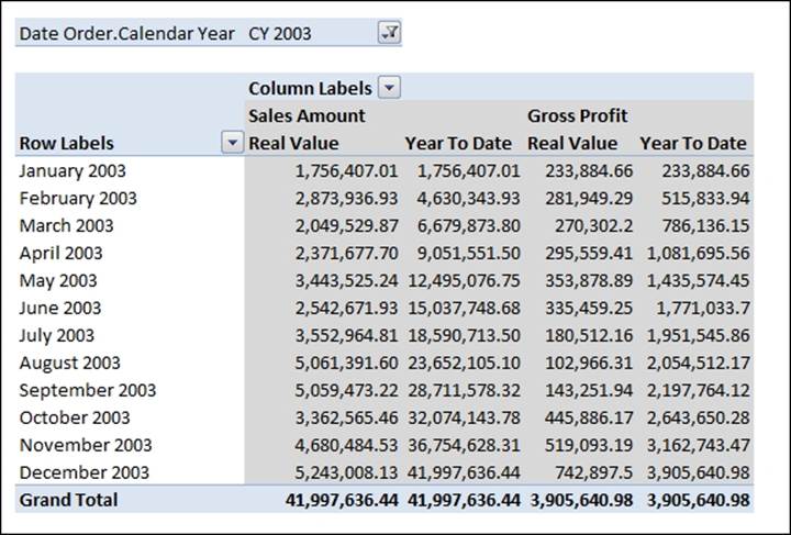
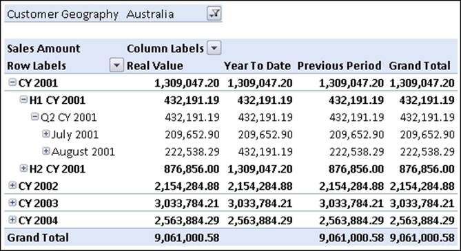
We can see from the screenshot that the Year-To-Date calculation works with both Sales Amount and Gross Profit, even though we did not write any specific code for the two measures. Moreover, the screenshot shows why the Real Value member is needed: it is the reference back to the original physical space of the cube, while Year To Date is the new virtual plane in the multidimensional space that holds the results of our calculation.
The Time Intelligence wizard
SQL Server Data Tools can build a calculation dimension automatically when we run the Add Business Intelligence wizard (found under the Cube menu) and choose the Define Time Intelligence option. Now that we understand the basic technique of how to build a Calculation Dimension – and the wizard uses, essentially, the same technique - we can take a look at what the wizard actually creates and understand its limitations. While Calculation Dimensions are a powerful tool, the way that the Time Intelligence Wizard implements them is seriously flawed and as a result our recommendation is that you do not use the wizard at all. We'll now explain why this is.
Attribute overwrite
The first issue is that the wizard creates a new hierarchy on an existing dimension to hold calculations, and this leads to some unexpected behavior. Once again, though, before trying to understand the theory let's take a look at what actually happens in practice.
Consider the following, very simple query:
SELECT
NON EMPTY {
([Date Order].[Calendar Date Order Calculations].[Current Date Order]),
([Date Order].[Calendar Date Order Calculations].[Previous Period])
} ON 0,
[Date Order].[Calendar].[Date].&[20010712] ON 1
FROM
Sales
WHERE
Measures.[Sales Amount]
The query returns the real member from the hierarchy that the Time Intelligence Wizard creates, Current Date Order, and the Previous Period calculated member, for the Sales Amount measure and July 12, 2001:
|
Current Date Order |
Previous Period |
|
|
July 12, 2001 |
14,134.80 |
14,313.08 |
However, if we rewrite the query using a calculated member, as in:
WITH
MEMBER Measures.SalesPreviousPeriod AS
([Measures].[Sales Amount],
[Date Order].[Calendar Date Order Calculations].[Previous Period])
SELECT
{
Measures.[Sales Amount],
SalesPreviousPeriod
} ON 0,
NON EMPTY
[Date Order].[Calendar].[Date].&[20010712]
ON 1
FROM
Sales
The result seems to be incorrect:
|
Current Date Order |
SalesPreviousPeriod |
|
|
July 12, 2001 |
14,134.80 |
NULL |
As we can see, the value of SalesPreviousPeriod is Null. This isn't a bug, and although it's hard to understand, there is a logical explanation for why this happens; it's certainly not what you or your users would expect to happen, though, and is likely to cause some complaints. This behavior is a result of the way attribute relationships within a dimension interact with each other; this is referred to as 'attribute overwrite', and you can read a full discussion of it here: http://tinyurl.com/AttributeOverwrite. There's also a discussion of how attribute overwrite causes this particular problem in the following blog entry: http://tinyurl.com/chrisattoverwrite.
Note
The easiest way to avoid this problem is to never implement a calculation dimension as a new hierarchy on an existing dimension.
Calculation dimensions should be implemented as new, standalone dimensions, and should not have any relationship with any other dimension.
Limitations of calculated members
As we have seen, a calculation dimension does not need to have a relationship with any fact table. Since all of the values on it will be calculated, there is no need to have any physical records to hold its data. So we might think that it's right that a calculation dimension should be made up of only calculated members.
Nevertheless, even if they appear to the end user exactly as real members, calculated members suffer some limitations in Analysis Services and we need to be well aware of them before trying to build a calculation dimension:
· Drillthrough does not work with calculated members. Even if they can be used to make up a set of coordinates to a cell in the cube, just like real members, Analysis Services will refuse to initiate a drillthrough action on a cell covered by a calculated member. Of course, even when we can do a drillthrough we still have the problem of getting it to return the results we'd expect, but that's a problem we'll deal with later.
· There are severe limitations in the security model for calculated members. These limitations will be described in a later chapter, but basically, you cannot secure a calculated member role. While you can use dimension security to secure a real member, you cannot hide the metadata associated with a calculated member.
· Some clients handle calculated members in a different way compared to real members. Even if this is a client tool limitation, we need to be aware of it because our users will always interact with a cube through a client tool and will not care whether the limitation is on the client or the server. The most important client tool that suffers from this problem is Excel 2007, which does not display calculated members on non-measures dimensions by default, and which in some circumstances forces you to select all or none of the calculated members on a hierarchy, rather than just the ones you need. In later versions of Excel, this issue has been solved.
Therefore, from the point of view of usability and flexibility, calculated members are second class citizens. We need to create a proper, physical structure as the basis for our calculation dimension. In other words, we need to create real members, not calculated ones.
Of course, we are not going to pre-calculate all of the values for our calculated members and store them in fact table. What we will do instead, is to fool Analysis Services creating a real member while, under the hood, we overwrite the value of that real member with the result of an MDX calculation.
Calculation dimension best practices
Now that we are confident with both the basic concept of a calculation dimension and how it should be built, let's now go through the process of building one in more detail, following the best practices we've mentioned.
The first step is to create a new physical dimension, with real members for each of the calculations we're going to need. We don't actually need to create a table in our data warehouse for this purpose, we can do this with an SQL view like this:
CREATE VIEW DateTool AS
SELECT ID_Calc = 1, Calc = 'Real Value'
UNION ALL
SELECT ID_Calc = 2, Calc = 'Year To Date'
UNION ALL
SELECT ID_Calc = 3, Calc = 'Previous Period'
This view contains three rows, one for each member we need.
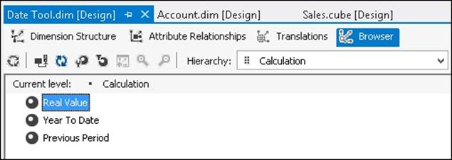
Next, we need to add this view to our DSV and create a dimension based on it. The dimension must have one hierarchy and this hierarchy must have its IsAggregatable property set to False: it makes no sense to have an All Member on it because the members on it should never be aggregated. The DefaultMember property of this hierarchy should then be set to the Real Value member. Giving this dimension a name can be quite difficult, as it should be something that helps the users understand what it does – here we've called it Date Tool, but other possibilities could be Time Calculations or Date Comparisons.
After it has been processed, the single hierarchy should look like this:
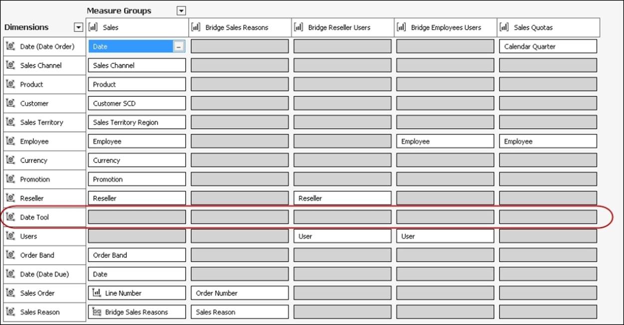
We now need to add it to the cube. What relationship should it have to the measure groups in the cube? In fact, it needs no relationship to any measure group at all to work:
At this point, if we query the cube using this new dimension, we'll see something like what's shown in the following screenshot:
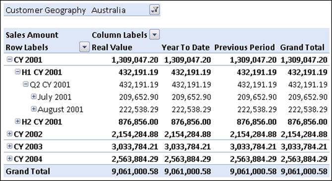
The PivotTable shows the same value for each member on the hierarchy, as there is no relationship between the dimension and any measure group.
Our next task is to overwrite the value returned by each member so that they return the calculations we want. We can do this using a simple SCOPE statement in the MDX Script of the cube:
SCOPE ([Date Tool].[Calculation].[Year To Date]);
THIS = AGGREGATE (
YTD ([Date Order].[Calendar].CurrentMember),
[Date Tool].[Calculation].[Real Value]);
END SCOPE;
If we now query the cube, with this calculation in place, we will get the result we want for the Year To Date member of the Date Tool dimension:
Note
A more complete, worked example of a Calculation Dimension, including many more calculations, is available here: http://tinyurl.com/datetool. In some cases, it can be useful to have more than one calculation dimension in the same cube so that the calculations can interact with each other – for example applying the same period previous year growth calculation to a year-to-date. This is discussed in the following blog entry: http://tinyurl.com/multicalcdims
Named sets
Another very interesting topic slightly related to calculated members is that of named sets. A named set is simply a set of members or tuples to which we assign a name. We define named sets to make it easier for users to build their queries, and also to help us as developers write more readable code.
Regular named sets
Let's take a look at an example of how named sets can be used. Our user might want to build an Excel report that shows detailed information about the sales of the current month, the sales of the previous one, and the total sales of the last three years. Without a named set, at each start of the month, the user would need to update the dates selected in the report in order to display the most recent month with data. In order to avoid having to do this, we can define a named set containing exactly the date range the user wants to see in the report that will never need manual updating. Here's how to do this:
First of all, since the Date Order dimension contains dates in the future that do not contain any sales, we first need to define the set of months where there are sales. This is easy to do using the NonEmpty function:
CREATE HIDDEN SET ExistingSalePeriods AS
NonEmpty (
[Date Order].[Calendar].[Month].Members,
Measures.[Sales Amount]
);
We define the set as HIDDEN because we do not want to make it visible to the user; we are only going to use it as an intermediate step towards constructing the set we want.
Next, since we are interested in the latest month where there are sales, we can simply define a new set that contains the last item in the ExistingSalePeriods:
CREATE SET LastSaleMonth AS
Tail (ExistingSalePeriods, 1);
This set, even if it is another step towards our ultimate goal, might be useful for the user to see, so we have left it visible. Our final set will contain members at the Year level, so we need to define a new set containing the latest year containing sales:
CREATE SET LastSaleYear AS
Ancestor (
LastSaleMonth.Item (0),
[Date Order].[Calendar].[Calendar Year]);
The last step is to create our final set:
CREATE SET LastSaleAnalysisPeriod AS
{
LastSaleYear.Item (0).Lag(2) :
LastSaleYear.Item (0),
LastSaleMonth.Item (0).PrevMember,
LastSaleMonth.Item (0)
};
Now that the set has been created, the user will be able to select the set in their client tool and use it in their report very easily:
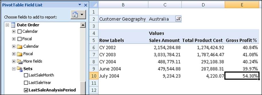
Named sets are evaluated and created every time the cube is processed, so as a result whenever a new month with sales appears in the data, the set will reflect this and the report will automatically show the required time periods when it is refreshed.
Dynamic named sets
As we've just seen, named sets are, by default, static – their contents will always stay the same until the next time the cube is processed. This is useful in some situations, for example, when you're trying to improve query performance, but in others it can be quite frustrating. Imagine, for example, we wanted to define a set containing our 10 best-selling products. We can easily build it using the TopCount function:
CREATE SET Best10Products AS
TopCount (
Product.Product.Product.Members,
10,
Measures.[Sales Amount]
);
Since this set is evaluated once, before any queries are run, it will contain the top-selling products for all time, for all customers, and so on. In other words, when the set is evaluated it knows nothing about any queries we might want to use it in. However, this set isn't much use for reporting: it's highly likely that there will be a different top-ten set of products for each month and each country, and if we wanted to build a report to show the top-ten products on rows with month and country on the slicer, we'd not be able to use a static named set. For example, the two following queries show the same list of products on rows – and in neither case do they show the top products for the years selected:
SELECT Measures.[Sales Amount] ON COLUMNS,
Best10Products ON ROWS
FROM
Sales
WHERE
([Date Order].[Calendar].[Calendar Year].&[2001])
SELECT Measures.[Sales Amount] ON COLUMNS,
Best10Products ON ROWS
FROM
Sales
WHERE
([Date Order].[Calendar].[Calendar Year].&[2004])
To handle this problem, Analysis Services 2008 introduced dynamic sets. Dynamic sets are evaluated once per query, in the context of the WHERE clause of that query. In order to make a static set dynamic, all we have to do is add the DYNAMIC keyword just before theSET definition, as in:
CREATE DYNAMIC SET Best10ProductsDynamic AS
TopCount (
Product.Product.Product.Members,
10,
Measures.[Sales Amount]
);
Now, if we run this query:
SELECT Measures.[Sales Amount] ON COLUMNS,
Best10ProductsDynamic ON ROWS
FROM
Sales
WHERE
([Date Order].[Calendar].[Calendar Year].&[2001])
SELECT Measures.[Sales Amount] ON COLUMNS,
Best10ProductsDynamic ON ROWS
FROM
Sales
WHERE
([Date Order].[Calendar].[Calendar Year].&[2004])
We get the correct set of top-ten products for each year.
However, dynamic sets are still quite limited in their uses because they are not completely aware of the context of the query they're being used in. For example, if a user tried to put several years on the rows axis of a query they would not be able to use a dynamic set to show the top-ten products for each year. Also, the way some client tools generate MDX (once again, Excel 2007 is the main offender here) means that dynamic sets will not work correctly with them. As a result, they should be used with care and users must be made aware of what they can and can't be used for.
Summary
In this chapter, we have seen many ways to enhance our cube by adding calculations to it. Let us briefly recall them:
· Calculated Measures create new measures whose value is calculated using MDX expressions. The new measures will be available as if they are real measures, although they do not support drillthrough.
· Calculation dimensions allow us to apply a single calculation to all of the measures in our cube, avoiding the need to create multiple calculated measures.
· Named sets allow us to predefine static or semi-static sets of members that in turn make building reports easier for our users.
In the next chapter, we'll move on to look at a much more complex, but nonetheless common type of calculation: currency conversion.