T-SQL Querying (2015)
Chapter 1. Logical query processing
Observing true experts in different fields, you find a common practice that they all share—mastering the basics. One way or another, all professions deal with problem solving. All solutions to problems, complex as they may be, involve applying a mix of fundamental techniques. If you want to master a profession, you need to build your knowledge upon strong foundations. Put a lot of effort into perfecting your techniques, master the basics, and you’ll be able to solve any problem.
This book is about Transact-SQL (T-SQL) querying—learning key techniques and applying them to solve problems. I can’t think of a better way to start the book than with a chapter on the fundamentals of logical query processing. I find this chapter the most important in the book—not just because it covers the essentials of query processing but also because SQL programming is conceptually very different than any other sort of programming.
![]() Note
Note
This book is in its third edition. The previous edition was in two volumes that are now merged into one. For details about the changes, plus information about getting the source code and sample data, make sure you visit the book’s introduction.
T-SQL is the Microsoft SQL Server dialect of, or extension to, the ANSI and ISO SQL standards. Throughout the book, I’ll use the terms SQL and T-SQL interchangeably. When discussing aspects of the language that originated from ANSI/ISO SQL and are relevant to most dialects, I’ll typically use the term SQL or standard SQL. When discussing aspects of the language with the implementation of SQL Server in mind, I’ll typically use the term T-SQL. Note that the formal language name is Transact-SQL, although it’s commonly called T-SQL. Most programmers, including myself, feel more comfortable calling it T-SQL, so I and the other authors made a conscious choice to use the term T-SQL throughout the book.
Origin of SQL pronunciation
Many English-speaking database professionals pronounce SQL as sequel, although the correct pronunciation of the language is S-Q-L (“ess kyoo ell”). One can make educated guesses about the reasoning behind the incorrect pronunciation. My guess is that there are both historical and linguistic reasons.
As for historical reasons, in the 1970s, IBM developed a language named SEQUEL, which was an acronym for Structured English QUEry Language. The language was designed to manipulate data stored in a database system named System R, which was based on Dr. Edgar F. Codd’s model for relational database management systems (RDBMS). The acronym SEQUEL was later shortened to SQL because of a trademark dispute. ANSI adopted SQL as a standard in 1986, and ISO did so in 1987. ANSI declared that the official pronunciation of the language is “ess kyoo ell,” but it seems that this fact is not common knowledge.
As for linguistic reasons, the sequel pronunciation is simply more fluent, mainly for English speakers. I often use it myself for this reason.
![]() More Info
More Info
The coverage of SQL history in this chapter is based on an article from Wikipedia, the free encyclopedia, and can be found at http://en.wikipedia.org/wiki/SQL.
SQL programming has many unique aspects, such as thinking in sets, the logical processing order of query elements, and three-valued logic. Trying to program in SQL without this knowledge is a straight path to lengthy, poor-performing code that is difficult to maintain. This chapter’s purpose is to help you understand SQL the way its designers envisioned it. You need to create strong roots upon which all the rest will be built. Where relevant, I’ll explicitly indicate elements that are specific to T-SQL.
Throughout the book, I’ll cover complex problems and advanced techniques. But in this chapter, as mentioned, I’ll deal only with the fundamentals of querying. Throughout the book, I’ll also focus on performance. But in this chapter, I’ll deal only with the logical aspects of query processing. I ask you to make an effort while reading this chapter not to think about performance at all. You’ll find plenty of performance coverage later in the book. Some of the logical query-processing phases that I’ll describe in this chapter might seem very inefficient. But keep in mind that in practice, the physical processing of a query in the database platform where it executes might be very different than the logical one.
The component in SQL Server in charge of generating the physical-query execution plan for a query is the query optimizer. In the plan, the optimizer determines in which order to access the tables, which access methods and indexes to use, which join algorithms to apply, and so on. The optimizer generates multiple valid execution plans and chooses the one with the lowest cost. The phases in the logical processing of a query have a specific order. In contrast, the optimizer can often make shortcuts in the physical execution plan that it generates. Of course, it will make shortcuts only if the result set is guaranteed to be the correct one—in other words, the same result set you would get by following the logical processing phases. For example, to use an index, the optimizer can decide to apply a filter much sooner than dictated by logical processing. I’ll refer to the processing order of the elements in the physical-query execution plan as physical processing order.
For the aforementioned reasons, you need to make a clear distinction between logical and physical processing of a query.
Without further ado, let’s delve into logical query-processing phases.
Logical query-processing phases
This section introduces the phases involved in the logical processing of a query. I’ll first briefly describe each step. Then, in the following sections, I’ll describe the steps in much more detail and apply them to a sample query. You can use this section as a quick reference whenever you need to recall the order and general meaning of the different phases.
Listing 1-1 contains a general form of a query, along with step numbers assigned according to the order in which the different clauses are logically processed.
LISTING 1-1 Logical query-processing step numbers
(5) SELECT (5-2) DISTINCT (7) TOP(<top_specification>) (5-1) <select_list>
(1) FROM (1-J) <left_table> <join_type> JOIN <right_table> ON <on_predicate>
| (1-A) <left_table> <apply_type> APPLY <right_input_table> AS <alias>
| (1-P) <left_table> PIVOT(<pivot_specification>) AS <alias>
| (1-U) <left_table> UNPIVOT(<unpivot_specification>) AS <alias>
(2) WHERE <where_predicate>
(3) GROUP BY <group_by_specification>
(4) HAVING <having_predicate>
(6) ORDER BY <order_by_list>
(7) OFFSET <offset_specification> ROWS FETCH NEXT <fetch_specification> ROWS ONLY;
The first noticeable aspect of SQL that is different from other programming languages is the logical order in which the code is processed. In most programming languages, the code is processed in the order in which it is written (call its typed order). In SQL, the first clause that is processed is the FROM clause, whereas the SELECT clause, which is typed first, is processed almost last. I refer to this order as logical processing order to distinguish it from both typed order and physical processing order.
There’s a reason for the difference between logical processing order and typed order. Remember that prior to SQL the language was named SEQUEL, and in the original name the first E stood for English. The designers of the language had in mind a declarative language where you declare your instructions in a language similar to English. Consider the manner in which you provide an instruction in English: “Bring me the T-SQL Querying book from the office.” You indicate the object (the book) before indicating the location of the object (the office). But clearly, the person carrying out the instruction would have to first go to the office, and then from there obtain the book. In a similar manner, in SQL the typed order indicates the SELECT clause with the desired columns before the FROM clause with the source tables. But logical query processing starts with the FROM clause. This realization tends to generate many a-ha moments for people, explaining so many things about SQL that might otherwise seem obscure.
Each step in logical query processing generates a virtual table that is used as the input to the following step. These virtual tables are not available to the caller (client application or outer query). Only the table generated by the final step is returned to the caller. If a certain clause is not specified in a query, the corresponding step is simply skipped. The following section briefly describes the different logical steps.
Logical query-processing phases in brief
Don’t worry too much if the description of the steps doesn’t seem to make much sense for now. These descriptions are provided as a reference. Sections that come after the scenario example will cover the steps in much more detail. Also, here I describe only the join table operator because it’s the most commonly used one and therefore easy to relate to. The other table operators (APPLY, PIVOT, and UNPIVOT) are covered later in the chapter in the section “Further aspects of logical query processing.”
Figure 1-1 contains a flow diagram representing logical query-processing phases in detail. Throughout the chapter, I’ll refer to the step numbers that appear in the diagram.
![]() (1) FROM This phase identifies the query’s source tables and processes table operators. Each table operator applies a series of subphases. For example, the phases involved in a join are (1-J1) Cartesian Product, (1-J2) ON Predicate, (1-J3) Add Outer Rows. This phase generates virtual table VT1.
(1) FROM This phase identifies the query’s source tables and processes table operators. Each table operator applies a series of subphases. For example, the phases involved in a join are (1-J1) Cartesian Product, (1-J2) ON Predicate, (1-J3) Add Outer Rows. This phase generates virtual table VT1.
![]() (1-J1) Cartesian Product This phase performs a Cartesian product (cross join) between the two tables involved in the table operator, generating VT1-J1.
(1-J1) Cartesian Product This phase performs a Cartesian product (cross join) between the two tables involved in the table operator, generating VT1-J1.
![]() (1-J2) ON Predicate This phase filters the rows from VT1-J1 based on the predicate that appears in the ON clause (<on_predicate>). Only rows for which the predicate evaluates to TRUE are inserted into VT1-J2.
(1-J2) ON Predicate This phase filters the rows from VT1-J1 based on the predicate that appears in the ON clause (<on_predicate>). Only rows for which the predicate evaluates to TRUE are inserted into VT1-J2.
![]() (1-J3) Add Outer Rows If OUTER JOIN is specified (as opposed to CROSS JOIN or INNER JOIN), rows from the preserved table or tables for which a match was not found are added to the rows from VT1-J2 as outer rows, generating VT1-J3.
(1-J3) Add Outer Rows If OUTER JOIN is specified (as opposed to CROSS JOIN or INNER JOIN), rows from the preserved table or tables for which a match was not found are added to the rows from VT1-J2 as outer rows, generating VT1-J3.
![]() (2) WHERE This phase filters the rows from VT1 based on the predicate that appears in the WHERE clause (<where_predicate>). Only rows for which the predicate evaluates to TRUE are inserted into VT2.
(2) WHERE This phase filters the rows from VT1 based on the predicate that appears in the WHERE clause (<where_predicate>). Only rows for which the predicate evaluates to TRUE are inserted into VT2.
![]() (3) GROUP BY This phase arranges the rows from VT2 in groups based on the set of expressions (aka, grouping set) specified in the GROUP BY clause, generating VT3. Ultimately, there will be one result row per qualifying group.
(3) GROUP BY This phase arranges the rows from VT2 in groups based on the set of expressions (aka, grouping set) specified in the GROUP BY clause, generating VT3. Ultimately, there will be one result row per qualifying group.
![]() (4) HAVING This phase filters the groups from VT3 based on the predicate that appears in the HAVING clause (<having_predicate>). Only groups for which the predicate evaluates to TRUE are inserted into VT4.
(4) HAVING This phase filters the groups from VT3 based on the predicate that appears in the HAVING clause (<having_predicate>). Only groups for which the predicate evaluates to TRUE are inserted into VT4.
![]() (5) SELECT This phase processes the elements in the SELECT clause, generating VT5.
(5) SELECT This phase processes the elements in the SELECT clause, generating VT5.
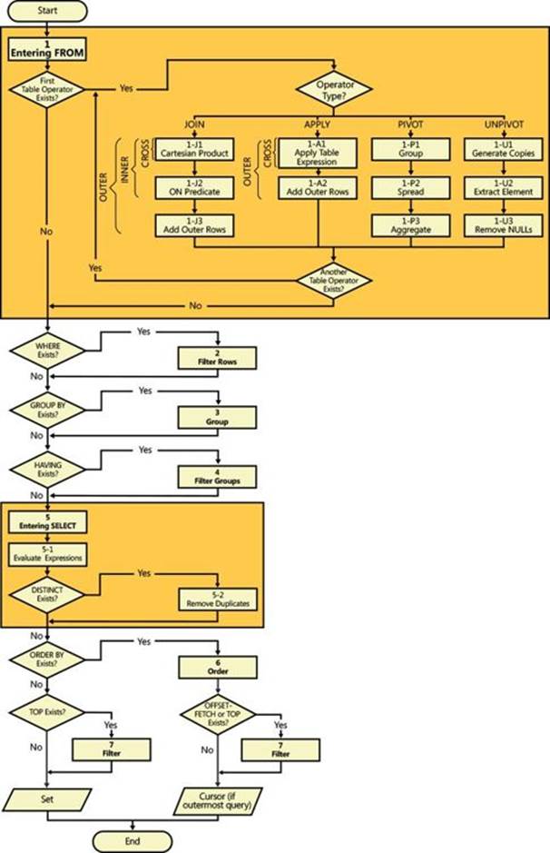
FIGURE 1-1 Logical query-processing flow diagram.
![]() (5-1) Evaluate Expressions This phase evaluates the expressions in the SELECT list, generating VT5-1.
(5-1) Evaluate Expressions This phase evaluates the expressions in the SELECT list, generating VT5-1.
![]() (5-2) DISTINCT This phase removes duplicate rows from VT5-1, generating VT5-2.
(5-2) DISTINCT This phase removes duplicate rows from VT5-1, generating VT5-2.
![]() (6) ORDER BY This phase orders the rows from VT5-2 according to the list specified in the ORDER BY clause, generating the cursor VC6. Absent an ORDER BY clause, VT5-2 becomes VT6.
(6) ORDER BY This phase orders the rows from VT5-2 according to the list specified in the ORDER BY clause, generating the cursor VC6. Absent an ORDER BY clause, VT5-2 becomes VT6.
![]() (7) TOP | OFFSET-FETCH This phase filters rows from VC6 or VT6 based on the top or offset-fetch specification, generating VC7 or VT7, respectively. With TOP, this phase filters the specified number of rows based on the ordering in the ORDER BY clause, or based on arbitrary order if an ORDER BY clause is absent. With OFFSET-FETCH, this phase skips the specified number of rows, and then filters the next specified number of rows, based on the ordering in the ORDER BY clause. The OFFSET-FETCH filter was introduced in SQL Server 2012.
(7) TOP | OFFSET-FETCH This phase filters rows from VC6 or VT6 based on the top or offset-fetch specification, generating VC7 or VT7, respectively. With TOP, this phase filters the specified number of rows based on the ordering in the ORDER BY clause, or based on arbitrary order if an ORDER BY clause is absent. With OFFSET-FETCH, this phase skips the specified number of rows, and then filters the next specified number of rows, based on the ordering in the ORDER BY clause. The OFFSET-FETCH filter was introduced in SQL Server 2012.
Sample query based on customers/orders scenario
To describe the logical processing phases in detail, I’ll walk you through a sample query. First run the following code to create the dbo.Customers and dbo.Orders tables, populate them with sample data, and query them to show their contents:
SET NOCOUNT ON;
USE tempdb;
IF OBJECT_ID(N'dbo.Orders', N'U') IS NOT NULL DROP TABLE dbo.Orders;
IF OBJECT_ID(N'dbo.Customers', N'U') IS NOT NULL DROP TABLE dbo.Customers;
CREATE TABLE dbo.Customers
(
custid CHAR(5) NOT NULL,
city VARCHAR(10) NOT NULL,
CONSTRAINT PK_Customers PRIMARY KEY(custid)
);
CREATE TABLE dbo.Orders
(
orderid INT NOT NULL,
custid CHAR(5) NULL,
CONSTRAINT PK_Orders PRIMARY KEY(orderid),
CONSTRAINT FK_Orders_Customers FOREIGN KEY(custid)
REFERENCES dbo.Customers(custid)
);
GO
INSERT INTO dbo.Customers(custid, city) VALUES
('FISSA', 'Madrid'),
('FRNDO', 'Madrid'),
('KRLOS', 'Madrid'),
('MRPHS', 'Zion' );
INSERT INTO dbo.Orders(orderid, custid) VALUES
(1, 'FRNDO'),
(2, 'FRNDO'),
(3, 'KRLOS'),
(4, 'KRLOS'),
(5, 'KRLOS'),
(6, 'MRPHS'),
(7, NULL );
SELECT * FROM dbo.Customers;
SELECT * FROM dbo.Orders;
This code generates the following output:
custid city
------ ----------
FISSA Madrid
FRNDO Madrid
KRLOS Madrid
MRPHS Zion
orderid custid
----------- ------
1 FRNDO
2 FRNDO
3 KRLOS
4 KRLOS
5 KRLOS
6 MRPHS
7 NULL
I’ll use the query shown in Listing 1-2 as my example. The query returns customers from Madrid who placed fewer than three orders (including zero orders), along with their order counts. The result is sorted by order count, from smallest to largest.
LISTING 1-2 Query: Madrid customers with fewer than three orders
SELECT C.custid, COUNT(O.orderid) AS numorders
FROM dbo.Customers AS C
LEFT OUTER JOIN dbo.Orders AS O
ON C.custid = O.custid
WHERE C.city = 'Madrid'
GROUP BY C.custid
HAVING COUNT(O.orderid) < 3
ORDER BY numorders;
This query returns the following output:
custid numorders
------ -----------
FISSA 0
FRNDO 2
Both FISSA and FRNDO are customers from Madrid who placed fewer than three orders. Examine the query and try to read it while following the steps and phases described in Listing 1-1, Figure 1-1, and the section “Logical query-processing phases in brief.” If this is your first time thinking of a query in such terms, you might be confused. The following section should help you understand the nitty-gritty details.
Logical query-processing phase details
This section describes the logical query-processing phases in detail by applying them to the given sample query.
Step 1: The FROM phase
The FROM phase identifies the table or tables that need to be queried, and if table operators are specified, this phase processes those operators from left to right. Each table operator operates on one or two input tables and returns an output table. The result of a table operator is used as the left input to the next table operator—if one exists—and as the input to the next logical query-processing phase otherwise. Each table operator has its own set of processing subphases. For example, the subphases involved in a join are (1-J1) Cartesian Product, (1-J2) ON Predicate, (1-J3) Add Outer Rows. As mentioned, other table operators will be described separately later in this chapter. The FROM phase generates virtual table VT1.
Step 1-J1: Perform Cartesian product (cross join)
This is the first of three subphases that are applicable to a join table operator. This subphase performs a Cartesian product (a cross join, or an unrestricted join) between the two tables involved in the join and, as a result, generates virtual table VT1-J1. This table contains one row for every possible choice of a row from the left table and a row from the right table. If the left table contains n rows and the right table contains m rows, VT1-J1 will contain n×m rows. The columns in VT1-J1 are qualified (prefixed) with their source table names (or table aliases, if you specified them in the query). In the subsequent steps (step 1-J2 and on), a reference to a column name that is ambiguous (appears in more than one input table) must be table-qualified (for example, C.custid). Specifying the table qualifier for column names that appear in only one of the inputs is optional (for example, O.orderid or just orderid).
Apply step 1-J1 to the sample query (shown in Listing 1-2):
FROM dbo.Customers AS C ... JOIN dbo.Orders AS O
As a result, you get the virtual table VT1-J1 (shown in Table 1-1) with 28 rows (4×7).
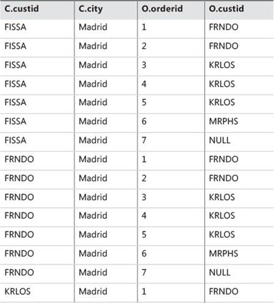
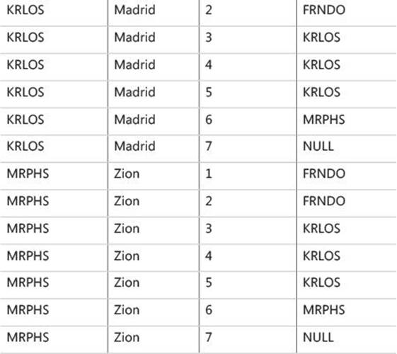
TABLE 1-1 Virtual table VT1-J1 returned from step 1-J1
Step 1-J2: Apply ON predicate (join condition)
The ON clause is the first of three query clauses (ON, WHERE, and HAVING) that filter rows based on a predicate. The predicate in the ON clause is applied to all rows in the virtual table returned by the previous step (VT1-J1). Only rows for which the <on_predicate> is TRUE become part of the virtual table returned by this step (VT1-J2).
NULLs and the three-valued logic
Allow me to digress a bit to cover some important aspects of SQL related to this step. The relational model defines two marks representing missing values: an A-Mark (missing and applicable) and an I-Mark (missing and inapplicable). The former represents a case where a value is generally applicable, but for some reason is missing. For example, consider the attribute birthdate of the People relation. For most people this information is known, but in some rare cases it isn’t, as my wife’s grandpa will attest. Obviously, he was born on some date, but no one knows which date it was. The latter represents a case where a value is irrelevant. For example, consider the attribute custid of the Orders relation. Suppose that when you perform inventory in your company, if you find inconsistency between the expected and actual stock levels of an item, you add a dummy order to the database to compensate for it. In such a transaction, the customer ID is irrelevant.
Unlike the relational model, the SQL standard doesn’t make a distinction between different kinds of missing values, rather it uses only one general-purpose mark—the NULL mark. NULLs are a source for quite a lot of confusion and trouble in SQL and should be understood well to avoid errors. For starters, a common mistake that people make is to use the term “NULL value,” but a NULL is not a value; rather, it’s a mark for a missing value. So the correct terminology is either “NULL mark” or just “NULL.” Also, because SQL uses only one mark for missing values, when you use a NULL, there’s no way for SQL to know whether it is supposed to represent a missing and applicable case or a missing and inapplicable case. For example, in our sample data one of the orders has a NULL mark in the custid column. Suppose that this is a dummy order that is not related to any customer like the scenario I described earlier. So your use of a NULL here records the fact that the value is missing, but not the fact that it’s missing and inapplicable.
A big part of the confusion in working with NULLs in SQL is related to predicates you use in query filters, CHECK constraints, and elsewhere. The possible values of a predicate in SQL are TRUE, FALSE, and UNKNOWN. This is referred to as three-valued logic and is unique to SQL. Logical expressions in most programming languages can be only TRUE or FALSE. The UNKNOWN logical value in SQL typically occurs in a logical expression that involves a NULL. (For example, the logical value of each of these three expressions is UNKNOWN:NULL > 1759; NULL = NULL; X + NULL > Y.) Remember that the NULL mark represents a missing value. According to SQL, when comparing a missing value to another value (even another NULL), the logical result is always UNKNOWN.
Dealing with UNKNOWN logical results and NULLs can be very confusing. While NOT TRUE is FALSE, and NOT FALSE is TRUE, the opposite of UNKNOWN (NOT UNKNOWN) is still UNKNOWN.
UNKNOWN logical results and NULLs are treated inconsistently in different elements of the language. For example, all query filters (ON, WHERE, and HAVING) treat UNKNOWN like FALSE. A row for which a filter is UNKNOWN is eliminated from the result set. In other words, query filters return TRUE cases. On the other hand, an UNKNOWN value in a CHECK constraint is actually treated like TRUE. Suppose you have a CHECK constraint in a table to require that the salary column be greater than zero. A row entered into the table with a NULL salary is accepted because (NULL > 0) is UNKNOWN and treated like TRUE in the CHECK constraint. In other words, CHECK constraints reject FALSE cases.
A comparison between two NULLs in a filter yields UNKNOWN, which, as I mentioned earlier, is treated like FALSE—as if one NULL is different than another.
On the other hand, for UNIQUE constraints, some relational operators, and sorting or grouping operations, NULLs are treated as equal:
![]() You cannot insert into a table two rows with a NULL in a column that has a UNIQUE constraint defined on it. T-SQL violates the standard on this point.
You cannot insert into a table two rows with a NULL in a column that has a UNIQUE constraint defined on it. T-SQL violates the standard on this point.
![]() A GROUP BY clause groups all NULLs into one group.
A GROUP BY clause groups all NULLs into one group.
![]() An ORDER BY clause sorts all NULLs together.
An ORDER BY clause sorts all NULLs together.
![]() The UNION, EXCEPT, and INTERSECT operators treat NULLs as equal when comparing rows from the two sets.
The UNION, EXCEPT, and INTERSECT operators treat NULLs as equal when comparing rows from the two sets.
Interestingly, the SQL standard doesn’t use the terms equal to and not equal to when describing the way the UNION, EXCEPT, and INTERSECT relational operators compare rows; rather, it uses is not distinct from and is distinct from, respectively. In fact, the standard defines an explicit distinct predicate using the form: IS [ NOT ] DISTINCT FROM. These relational operators use the distinct predicate implicitly. It differs from predicates using = and <> operators in that it uses two-valued logic. The following expressions are true: NULL IS NOT DISTINCT FROM NULL, NULL IS DISTINCT FROM 1759. As of SQL Server 2014, T-SQL doesn’t support the explicit distinct predicate, but I hope very much that such support will be added in the future. (See the feature request:http://connect.microsoft.com/SQLServer/feedback/details/286422/.)
In short, to spare yourself some grief you should be aware of the way UNKNOWN logical results and NULLs are treated in the different elements of the language.
Apply step 1-J2 to the sample query:
ON C.custid = O.custid
The first column of Table 1-2 shows the value of the logical expression in the ON clause for the rows from VT1-J1.
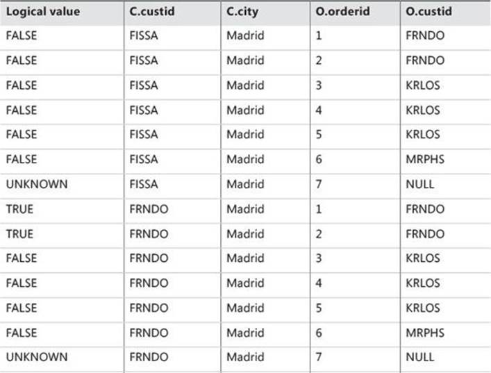
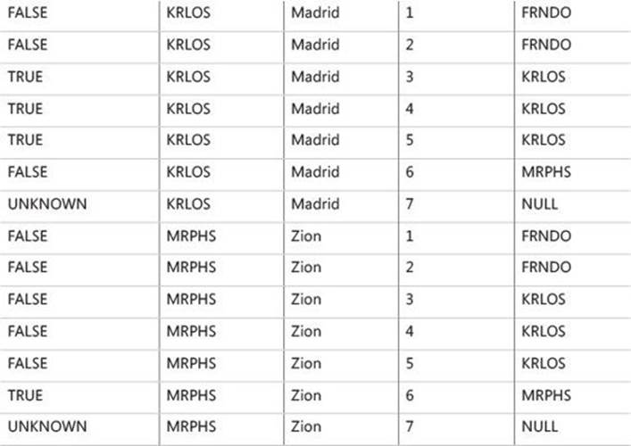
TABLE 1-2 Logical value of ON predicate for rows from VT1-J1
Only rows for which the <on_predicate> is TRUE are inserted into VT1-J2, as shown in Table 1-3.
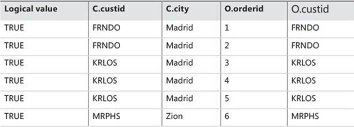
TABLE 1-3 Virtual table VT1-J2 returned from step 1-J2
Step 1-J3: Add outer rows
This step occurs only for an outer join. For an outer join, you mark one or both input tables as preserved by specifying the type of outer join (LEFT, RIGHT, or FULL). Marking a table as preserved means you want all its rows returned, even when filtered out by the <on_predicate>. A left outer join marks the left table as preserved, a right outer join marks the right one, and a full outer join marks both. Step 1-J3 returns the rows from VT1-J2, plus rows from the preserved table or tables for which a match was not found in step 1-J2. These added rows are referred to as outer rows. NULLs are assigned to the attributes of the nonpreserved table in the outer rows. As a result, virtual table VT1-J3 is generated.
In our example, the preserved table is Customers:
Customers AS C LEFT OUTER JOIN Orders AS O
Only customer FISSA did not yield any matching orders (and thus wasn’t part of VT1-J2). Therefore, a row for FISSA is added to VT1-J2, with NULLs for the Orders attributes. The result is virtual table VT1-J3 (shown in Table 1-4). Because the FROM clause of the sample query has no more table operators, the virtual table VT1-J3 is also the virtual table VT1 returned from the FROM phase.
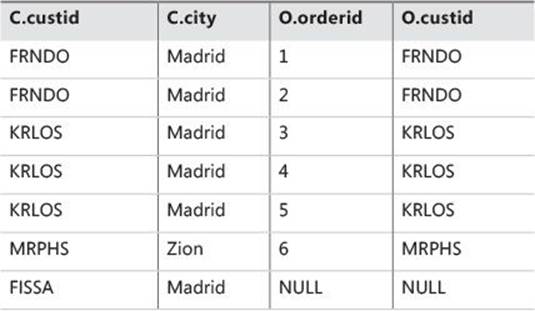
TABLE 1-4 Virtual table VT1-J3 (also VT1) returned from step 1-J3
![]() Note
Note
If multiple table operators appear in the FROM clause, they are processed from left to right—that’s at least the case in terms of the logical query-processing order. The result of each table operator is provided as the left input to the next table operator. The final virtual table will be used as the input for the next step.
Step 2: The WHERE phase
The WHERE filter is applied to all rows in the virtual table returned by the previous step. Those rows for which <where_predicate> is TRUE make up the virtual table returned by this step (VT2).
![]() Caution
Caution
You cannot refer to column aliases created by the SELECT list because the SELECT list was not processed yet—for example, you cannot write SELECT YEAR(orderdate) AS orderyear ... WHERE orderyear > 2014. Ironically, some people think that this behavior is a bug in SQL Server, but it can be easily explained when you understand logical query processing. Also, because the data is not yet grouped, you cannot use grouped aggregates here—for example, you cannot write WHERE orderdate = MAX(orderdate).
Apply the filter in the sample query:
WHERE C.city = 'Madrid'
The row for customer MRPHS from VT1 is removed because the city is not Madrid, and virtual table VT2, which is shown in Table 1-5, is generated.
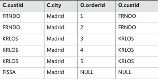
TABLE 1-5 Virtual table VT2 returned from step 2
A confusing aspect of queries containing outer joins is whether to specify a predicate in the ON clause or in the WHERE clause. The main difference between the two is that ON is applied before adding outer rows (step 1-J3), whereas WHERE is applied afterward. An elimination of a row from the preserved table by the ON clause is not final because step 1-J3 will add it back; an elimination of a row by the WHERE clause, by contrast, is final. Another way to look at it is to think of the ON predicate as serving a matching purpose, and of the WHERE predicate as serving a more basic filtering purpose. Regarding the rows from the preserved side of the join, the ON clause cannot discard those; it can only determine which rows from the nonpreserved side to match them with. However, the WHERE clause can certainly discard rows from the preserved side. Bearing this in mind should help you make the right choice.
For example, suppose you want to return certain customers and their orders from the Customers and Orders tables. The customers you want to return are only Madrid customers—both those who placed orders and those who did not. An outer join is designed exactly for such a request. You perform a left outer join between Customers and Orders, marking the Customers table as the preserved table. To be able to return customers who placed no orders, you must specify the correlation between Customers and Orders in the ON clause (ON C.custid = O.custid). Customers with no orders are eliminated in step 1-J2 but added back in step 1-J3 as outer rows. However, because you want to return only Madrid customers, you must specify the city predicate in the WHERE clause (WHERE C.city = ‘Madrid’). Specifying the city predicate in the ON clause would cause non-Madrid customers to be added back to the result set by step 1-J3.
![]() Tip
Tip
This logical difference between the ON and WHERE clauses exists only when using an outer join. When you use an inner join, it doesn’t matter where you specify your predicate because step 1-J3 is skipped. The predicates are applied one after the other with no intermediate step between them, both serving a basic filtering purpose.
Step 3: The GROUP BY phase
The GROUP BY phase associates rows from the table returned by the previous step to groups according to the grouping set, or sets, defined in the GROUP BY clause. For simplicity, assume that you have a single set of expressions to group by. This set is called the grouping set.
In this phase, the rows from the table returned by the previous step are arranged in groups. Each unique combination of values of the expressions that belong to the grouping set identifies a group. Each row from the previous step is associated with one and only one group. Virtual table VT3 consists of the rows of VT2 arranged in groups (the raw information) along with the group identifiers (the groups information).
Apply step 3 to the following sample query:
GROUP BY C.custid
You get the virtual table VT3 shown in Table 1-6.
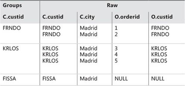
TABLE 1-6 Virtual table VT3 returned from step 3
Eventually, a grouped query will generate one row per group (unless that group is filtered out). Consequently, when GROUP BY is specified in a query, all subsequent steps (HAVING, SELECT, and so on) can specify only expressions that result in a scalar (singular) value per group. These expressions can include columns or expressions from the GROUP BY list—such as C.custid in the sample query here—or aggregate functions, such as COUNT(O.orderid).
Examine VT3 in Table 1-6 and think what the query should return for customer FRNDO’s group if the SELECT list you specify is SELECT C.custid, O.orderid. There are two different orderid values in the group; therefore, the answer is not a scalar. SQL doesn’t allow such a request. On the other hand, if you specify SELECT C.custid, COUNT(O.orderid) AS numorders, the answer for FRNDO is a scalar: it’s 2.
This phase considers NULLs as equal. That is, all NULLs are grouped into one group, just like a known value.
Step 4: The HAVING phase
The HAVING filter is applied to the groups in the table returned by the previous step. Only groups for which the <having_predicate> is TRUE become part of the virtual table returned by this step (VT4). The HAVING filter is the only filter that applies to the grouped data.
Apply this step to the sample query:
HAVING COUNT(O.orderid) < 3
The group for KRLOS is removed because it contains three orders. Virtual table VT4, which is shown in Table 1-7, is generated.
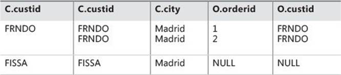
TABLE 1-7 Virtual table VT4 returned from step 4
![]() Note
Note
You must specify COUNT(O.orderid) here and not COUNT(*). Because the join is an outer one, outer rows were added for customers with no orders. COUNT(*) would have added outer rows to the count, undesirably producing a count of one order for FISSA. COUNT(O.orderid)correctly counts the number of orders for each customer, producing the desired value 0 for FISSA. Remember that COUNT(<expression>) ignores NULLs just like any other aggregate function.
![]() Note
Note
An aggregate function does not accept a subquery as an input—for example, HAVING SUM((SELECT ...)) > 10.
Step 5: The SELECT phase
Though specified first in the query, the SELECT clause is processed only at the fifth step. The SELECT phase constructs the table that will eventually be returned to the caller. This phase involves two subphases: (5-1) Evaluate Expressions and (5-2) Apply DISTINCT Clause.
Step 5-1: Evaluate expressions
The expressions in the SELECT list can return columns and manipulations of columns from the virtual table returned by the previous step. Remember that if the query is an aggregate query, after step 3 you can refer to columns from the previous step only if they are part of the groups section (GROUP BY list). If you refer to columns from the raw section, they must be aggregated. Nonmanipulated columns selected from the previous step maintain their original names unless you alias them (for example, col1 AS c1). Expressions involving manipulations of columns should be aliased to have a column name in the result table—for example, YEAR(orderdate) AS orderyear.
![]() Important
Important
As mentioned earlier, aliases created by the SELECT list cannot be used by earlier steps—for example, in the WHERE phase. When you understand the logical processing order of the query clauses, this makes perfect sense. In addition, expression aliases cannot even be used by other expressions within the same SELECT list. The reasoning behind this limitation is another unique aspect of SQL; many operations are all-at-once operations. For example, in the following SELECT list, the logical order in which the expressions are evaluated should not matter and is not guaranteed: SELECT c1 + 1 AS e1, c2 + 1 AS e2. Therefore, the following SELECT list is not supported: SELECT c1 + 1 AS e1, e1 + 1 AS e2. You’re allowed to use column aliases only in steps following the step that defined them. If you define a column alias in the SELECT phase, you can refer to that alias in the ORDER BY phase—for example, SELECT YEAR(orderdate) AS orderyear ... ORDER BY orderyear.
The concept of an all-at-once operation can be hard to grasp. For example, in most programming environments, to swap values between variables you use a temporary variable. However, to swap table column values in SQL, you can use the following:
UPDATE dbo.T1 SET c1 = c2, c2 = c1;
Logically, you should assume that the whole operation takes place at once. It is as if the source table is not modified until the whole operation finishes and then the result replaces the source. For similar reasons, the following UPDATE would update all of T1’s rows, adding to c1 the same maximum c1 value from T1 when the update started:
UPDATE dbo.T1 SET c1 = c1 + (SELECT MAX(c1) FROM dbo.T1);
Don’t be concerned that the maximum c1 value might keep changing as the operation proceeds; it does not because the operation occurs all at once.
Apply this step to the sample query:
SELECT C.custid, COUNT(O.orderid) AS numorders
You get the virtual table VT5-1, which is shown in Table 1-8. Because the other possible subphase (DISTINCT) of the SELECT phase isn’t applied in the sample query, the virtual table VT5-1 returned by this subphase is also the virtual table VT5 returned by the SELECT phase.
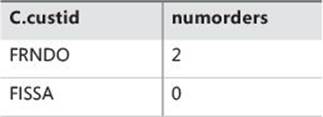
TABLE 1-8 Virtual table VT5-1 (also VT5) returned from step 5
Step 5-2: Apply the DISTINCT clause
If a DISTINCT clause is specified in the query, duplicate rows are removed from the virtual table returned by the previous step, and virtual table VT5-2 is generated.
![]() Note
Note
SQL deviates from the relational model by allowing a table to have duplicate rows (when a primary key or unique constraint is not enforced) and a query to return duplicate rows in the result. According to the relational model, the body of a relation is a set of tuples (what SQL callsrows), and according to mathematical set theory, a set (as opposed to a multiset) has no duplicates. Using the DISTINCT clause, you can ensure that a query returns unique rows and, in this sense, conform to the relational model.
You should realize that the SELECT phase first evaluates expressions (subphase 5-1) and only afterward removes duplicate rows (subphase 5-2). If you don’t realize this, you might be surprised by the results of some queries. As an example, the following query returns distinct customer IDs of customers who placed orders:
SELECT DISTINCT custid
FROM dbo.Orders
WHERE custid IS NOT NULL;
As you probably expected, this query returns three rows in the result set:
custid
------
FRNDO
KRLOS
MRPHS
Suppose you wanted to add row numbers to the result rows based on custid ordering. Not realizing the problem, you add to the query an expression based on the ROW_NUMBER function, like so (don’t run the query yet):
SELECT DISTINCT custid, ROW_NUMBER() OVER(ORDER BY custid) AS rownum
FROM dbo.Orders
WHERE custid IS NOT NULL;
Before you run the query, how many rows do you expect to get in the result? If your answer is 3, you’re wrong. That’s because phase 5-1 evaluates all expressions, including the one based on the ROW_NUMBER function, before duplicates are removed. In this example, the SELECT phase operates on table VT4, which has five rows (after the WHERE filter was applied). Therefore, phase 5-1 generates a table VT5-1 with five rows with row numbers 1 through 5. Including the row numbers, those rows are already unique. So when phase 5-2 is applied, it finds no duplicates to remove. Here’s the result of this query:
custid rownum
------ --------------------
FRNDO 1
FRNDO 2
KRLOS 3
KRLOS 4
KRLOS 5
MRPHS 6
If you want to assign row numbers to distinct customer IDs, you have to get rid of duplicate customer IDs before you assign the row numbers. This can be achieved by using a table expression such as a common table expression (CTE), like so:
WITH C AS
(
SELECT DISTINCT custid
FROM dbo.Orders
WHERE custid IS NOT NULL
)
SELECT custid, ROW_NUMBER() OVER(ORDER BY custid) AS rownum
FROM C;
This time you do get the desired output:
custid rownum
------ --------------------
FRNDO 1
KRLOS 2
MRPHS 3
Back to our original sample query from Listing 1-2, step 5-2 is skipped because DISTINCT is not specified. In this query, it would remove no rows anyway.
Step 6: The ORDER BY phase
The rows from the previous step are sorted according to the column list specified in the ORDER BY clause, returning the cursor VC6. The ORDER BY clause is the only step where column aliases created in the SELECT phase can be reused.
If DISTINCT is specified, the expressions in the ORDER BY clause have access only to the virtual table returned by the SELECT phase (VT5). If DISTINCT is not specified, expressions in the ORDER BY clause can access both the input and the output virtual tables of the SELECT phase (VT4 and VT5). Moreover, if DISTINCT isn’t present, you can specify in the ORDER BY clause any expression that would have been allowed in the SELECT clause. Namely, you can sort by expressions that you don’t end up returning in the final result set.
There is a reason for not allowing access to expressions you’re not returning if DISTINCT is specified. When adding expressions to the SELECT list, DISTINCT can potentially change the number of rows returned. Without DISTINCT, of course, changes in the SELECT list don’t affect the number of rows returned.
In our example, because DISTINCT is not specified, the ORDER BY clause has access to both VT4, shown in Table 1-7, and VT5, shown in Table 1-8.
In the ORDER BY clause, you can also specify ordinal positions of result columns from the SELECT list. For example, the following query sorts the orders first by custid and then by orderid:
SELECT orderid, custid FROM dbo.Orders ORDER BY 2, 1;
However, this practice is not recommended because you might make changes to the SELECT list and forget to revise the ORDER BY list accordingly. Also, when the query strings are long, it’s hard to figure out which item in the ORDER BY list corresponds to which item in the SELECT list.
![]() Important
Important
This step is different than all other steps in the sense that it doesn’t return a relational result; instead, it returns a cursor. Remember that the relational model is based on set theory, and that the body of a relation (what SQL calls a table) is a set of tuples (rows). The elements of a set have no particular order. A query with a presentation ORDER BY clause returns a result with rows organized in a particular order. Standard SQL calls such a result a cursor. Understanding this is one of the most fundamental steps to correctly understanding SQL.
When describing the contents of a table, most people (including me) routinely depict the rows in a certain order. But because a table is a set of rows with no particular order, such depiction can cause some confusion by implying otherwise. Figure 1-2 shows an example for depicting the content of tables in a more correct way that doesn’t imply order.
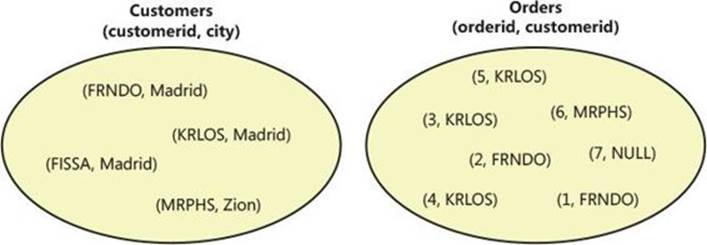
FIGURE 1-2 Customers and Orders sets.
![]() Note
Note
Although SQL doesn’t assume any given order to a table’s rows, it does maintain ordinal positions for columns based on creation order. Specifying SELECT * (although it’s a bad practice for several reasons I’ll describe later in the book) guarantees the columns would be returned in creation order. In this respect, SQL deviates from the relational model.
Because this step doesn’t return a table (it returns a cursor), a query with an ORDER BY clause that serves only a presentation ordering purpose cannot be used to define a table expression—that is, a view, an inline table-valued function, a derived table, or a CTE. Rather, the result must be consumed by a target that can handle the records one at a time, in order. Such a target can be a client application, or T-SQL code using a CURSOR object. An attempt to consume a cursor result by a target that expects a relational input will fail. For example, the following attempt to define a derived table is invalid and produces an error:
SELECT orderid, custid
FROM ( SELECT orderid, custid
FROM dbo.Orders
ORDER BY orderid DESC ) AS D;
Similarly, the following attempt to define a view is invalid:
CREATE VIEW dbo.MyOrders
AS
SELECT orderid, custid
FROM dbo.Orders
ORDER BY orderid DESC;
GO
There is an exceptional case in which T-SQL allows defining a table expression based on a query with an ORDER BY clause—when the query also specifies the TOP or OFFSET-FETCH filter. I’ll explain this exceptional case shortly after describing these filters.
The ORDER BY clause considers NULLs as equal. That is, NULLs are sorted together. Standard SQL leaves the question of whether NULLs are sorted lower or higher than known values up to implementations, which must be consistent. T-SQL sorts NULLs as lower than known values (first).
Apply this step to the sample query from Listing 1-2:
ORDER BY numorders
You get the cursor VC6 shown in Table 1-9.
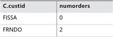
TABLE 1-9 Cursor VC6 returned from step 6
Step 7: Apply the TOP or OFFSET-FETCH filter
TOP and OFFSET-FETCH are query filters that are based on a count of rows and order. This is in contrast to the more classic query filters (ON, WHERE, and HAVING), which are based on a predicate. TOP is a T-SQL specific filter, whereas OFFSET-FETCH is standard. As mentioned, OFFSET-FETCH was introduced in SQL Server 2012. This section describes these filters in the context of logical query processing.
The TOP filter involves two elements in its specification. One (required) is the number or percentage of rows (rounded up) to be filtered. The other (optional) is the order defining which rows to filter. Unfortunately, the ordering specification for TOP (and the same goes for OFFSET-FETCH) is defined by the classic presentation ORDER BY clause in the query, as opposed to being disconnected from it and independent of it. I’ll explain in a moment why this design choice is problematic and leads to confusion. If order is not specified, you should assume it to be arbitrary, yielding a nondeterministic result. This means that if you run the query multiple times, you’re not guaranteed to get repeatable results even if the underlying data remains unchanged. Virtual table VT7 is generated. If the order is specified, cursor VC7 is generated. As an example, the following query returns the three orders with the highest orderid values:
SELECT TOP (3) orderid, custid
FROM dbo.Orders
ORDER BY orderid DESC;
This query generates the following output:
orderid custid
----------- ------
7 NULL
6 MRPHS
5 KRLOS
Even when order is specified, this fact alone doesn’t guarantee determinism. If the ordering isn’t unique (for example, if you change orderid in the preceding query to custid), the order between rows with the same sort values should be considered arbitrary. There are two ways to make a TOP filter deterministic. One is to specify a unique ORDER BY list (for example, custid, orderid). Another is to use a non-unique ORDER BY list and add the WITH TIES option. This option causes the filter to include also all other rows from the underlying query result that have the same sort values as the last row returned. With this option, the choice of which rows to return becomes deterministic, but the presentation ordering still isn’t in terms of rows with the same sort values.
The OFFSET-FETCH filter is similar to TOP, but it adds the option to indicate how many rows to skip (OFFSET clause) before indicating how many rows to filter (FETCH clause). Both the OFFSET and FETCH clauses are specified after the mandatory ORDER BY clause. As an example, the following query specifies the order based on orderid, descending, and it skips four rows and filters the next two rows:
SELECT orderid, custid
FROM dbo.Orders
ORDER BY orderid DESC
OFFSET 4 ROWS FETCH NEXT 2 ROWS ONLY;
This query returns the following output:
orderid custid
----------- ------
3 KRLOS
2 FRNDO
As of SQL Server 2014, the implementation of OFFSET-FETCH in T-SQL doesn’t yet support the PERCENT and WITH TIES options even though standard SQL does. This step generates cursor VC7.
Step 7 is skipped in our example because TOP and OFFSET-FETCH are not specified.
I mentioned earlier that the ordering for TOP and OFFSET-FETCH is defined by the same ORDER BY clause that traditionally defines presentation ordering, and that this causes confusion. Consider the following query as an example:
SELECT TOP (3) orderid, custid
FROM dbo.Orders
ORDER BY orderid DESC;
Here the ORDER BY clause serves two different purposes. One is the traditional presentation ordering (present the returned rows based on orderid, descending ordering). The other is to define for the TOP filter which three rows to pick (the three rows with the highest orderid values). But things get confusing if you want to define a table expression based on such a query. Recall from the section “Step 6: The ORDER BY phase,” that normally you are not allowed to define a table expression based on a query with an ORDER BY clause because such a query generates a cursor. I demonstrated attempts to define a derived table and a view that failed because the inner query had an ORDER BY clause.
There is an exception to this restriction, but it needs to be well understood to avoid incorrect expectations. The exception says that the inner query is allowed to have an ORDER BY clause to support a TOP or OFFSET-FETCH filter. But what’s important to remember in such a case is that if the outer query doesn’t have a presentation ORDER BY clause, the presentation ordering of the result is not guaranteed. The ordering is relevant only for the immediate query that contains the ORDER BY clause. If you want to guarantee presentation ordering of the result, the outermost query must include an ORDER BY clause. Here’s the exact language in the standard that indicates this fact, from ISO/IEC 9075-2:2011(E), section 4.15.3 Derived Tables:
A <query expression> can contain an optional <order by clause>. The ordering of the rows of the table specified by the <query expression> is guaranteed only for the <query expression> that immediately contains the <order by clause>.
Despite what you observe in practice, in the following example presentation ordering of the result is not guaranteed because the outermost query doesn’t have an ORDER BY clause:
SELECT orderid, custid
FROM ( SELECT TOP (3) orderid, custid
FROM dbo.Orders
ORDER BY orderid DESC ) AS D;
Suppose you run the preceding query and get a result that seems to be sorted in accordance with the inner query’s ordering specification. It doesn’t mean that the behavior is guaranteed to be repeatable. It could be a result of optimization aspects, and those are not guaranteed to be repeatable. This is one of the most common traps that SQL practitioners fall into—drawing a conclusion and basing expectations on observed behavior as opposed to correctly understanding the theory.
Along similar lines, a common mistake that people make is to attempt to create a “sorted view.” Remember that if you specify the TOP or OFFSET-FETCH options, you are allowed to include an ORDER BY clause in the inner query. So one way some try to achieve this without actually filtering rows is to specify the TOP (100) PERCENT option, like so:
-- Attempt to create a sorted view
IF OBJECT_ID(N'dbo.MyOrders', N'V') IS NOT NULL DROP VIEW dbo.MyOrders;
GO
-- Note: This does not create a "sorted view"!
CREATE VIEW dbo.MyOrders
AS
SELECT TOP (100) PERCENT orderid, custid
FROM dbo.Orders
ORDER BY orderid DESC;
GO
Consider the following query against the view:
SELECT orderid, custid FROM dbo.MyOrders;
According to what I just explained, if you query such a view and do not specify an ORDER BY clause in the outer query, you don’t get any presentation ordering assurances. When I ran this query on my system, I got the result in the following order:
orderid custid
----------- ------
1 FRNDO
2 FRNDO
3 KRLOS
4 KRLOS
5 KRLOS
6 MRPHS
7 NULL
As you can see, the result wasn’t returned based on orderid, descending ordering. Here the SQL Server query optimizer was smart enough to realize that because the outer query doesn’t have an ORDER BY clause, and TOP (100) PERCENT doesn’t really filter any rows, it can ignore both the filter and its ordering specification.
Another attempt to create a sorted view is to specify an OFFSET clause with 0 rows and omit the FETCH clause, like so:
-- Attempt to create a sorted view
IF OBJECT_ID(N'dbo.MyOrders', N'V') IS NOT NULL DROP VIEW dbo.MyOrders;
GO
-- Note: This does not create a "sorted view"!
CREATE VIEW dbo.MyOrders
AS
SELECT orderid, custid
FROM dbo.Orders
ORDER BY orderid DESC
OFFSET 0 ROWS;
GO
-- Query view
SELECT orderid, custid FROM dbo.MyOrders;
When I ran this query on my system, I got the result in the following order:
orderid custid
----------- ------
7 NULL
6 MRPHS
5 KRLOS
4 KRLOS
3 KRLOS
2 FRNDO
1 FRNDO
The result seems to be sorted by orderid, descending, but you still need to remember that this is not guaranteed behavior. It’s just that with this case the optimizer doesn’t have logic embedded in it yet to ignore the filter with its ordering specification like in the previous case.
All this confusion can be avoided if the filters are designed with their own ordering specification, independent of, and disconnected from, the presentation ORDER BY clause. An example for a good design that makes this separation is that of window functions like ROW_NUMBER. You specify the order for the ranking calculation, independent of any ordering that you may or may not want to define in the query for presentation purposes. But alas, for TOP and OFFSET-FETCH, that ship has sailed already. So the responsibility is now on us, the users, to understand the existing design well, and to know what to expect from it, and more importantly, what not to expect from it.
When you’re done, run the following code for cleanup:
IF OBJECT_ID(N'dbo.MyOrders', N'V') IS NOT NULL DROP VIEW dbo.MyOrders;
Further aspects of logical query processing
This section covers further aspects of logical query processing, including table operators (JOIN, APPLY, PIVOT, and UNPIVOT), window functions, and additional relational operators (UNION, EXCEPT, and INTERSECT). Note that I could say much more about these language elements besides their logical query-processing aspects, but that’s the focus of this chapter. Also, if a language element described in this section is completely new to you (for example, PIVOT, UNPIVOT, or APPLY), it might be a bit hard to fully comprehend its meaning at this point. Later in the book, I’ll conduct more detailed discussions, including uses, performance aspects, and so on. You can then return to this chapter and read about the logical query-processing aspects of that language element again to better comprehend its meaning.
Table operators
T-SQL supports four table operators in the FROM clause of a query: JOIN, APPLY, PIVOT, and UNPIVOT.
![]() Note
Note
APPLY, PIVOT, and UNPIVOT are not standard operators; rather, they are extensions specific to T-SQL. APPLY has a similar parallel in the standard called LATERAL, but PIVOT and UNPIVOT don’t.
I covered the logical processing phases involved with joins earlier. Here I’ll briefly describe the other three operators and the way they fit in the logical query-processing model.
Table operators get one or two tables as inputs. Call them left input and right input based on their position with respect to the table operator keyword (JOIN, APPLY, PIVOT, UNPIVOT). An input table could be, without being restricted, one of many options: a regular table, a temporary table, table variable, derived table, CTE, view, or table-valued function. In logical query-processing terms, table operators are evaluated from left to right, with the virtual table returned by one table operator becoming the left input table of the next table operator.
Each table operator involves a different set of steps. For convenience and clarity, I’ll prefix the step numbers with the initial of the table operator (J for JOIN, A for APPLY, P for PIVOT, and U for UNPIVOT).
Following are the four table operators along with their elements:
(J) <left_input_table>
{CROSS | INNER | OUTER} JOIN <right_input_table>
ON <on_predicate>
(A) <left_input_table>
{CROSS | OUTER} APPLY <right_input_table>
(P) <left_input_table>
PIVOT (<aggregate_func(<aggregation_element>)> FOR
<spreading_element> IN(<target_col_list>))
AS <result_table_alias>
(U) <left_input_table>
UNPIVOT (<target_values_col> FOR
<target_names_col> IN(<source_col_list>))
AS <result_table_alias>
As a reminder, a join involves a subset (depending on the join type) of the following steps:
![]() J1: Apply Cartesian Product
J1: Apply Cartesian Product
![]() J2: Apply ON Predicate
J2: Apply ON Predicate
![]() J3: Add Outer Rows
J3: Add Outer Rows
APPLY
The APPLY operator (depending on the apply type) involves one or both of the following two steps:
1. A1: Apply Right Table Expression to Left Table Rows
2. A2: Add Outer Rows
The APPLY operator applies the right table expression to every row from the left input. The right table expression can refer to the left input’s columns. The right input is evaluated once for each row from the left. This step unifies the sets produced by matching each left row with the corresponding rows from the right table expression, and this step returns the combined result.
Step A1 is applied in both CROSS APPLY and OUTER APPLY. Step A2 is applied only for OUTER APPLY. CROSS APPLY doesn’t return an outer (left) row if the inner (right) table expression returns an empty set for it. OUTER APPLY will return such a row, with NULLs as placeholders for the inner table expression’s attributes.
For example, the following query returns the two orders with the highest order IDs for each customer:
SELECT C.custid, C.city, A.orderid
FROM dbo.Customers AS C
CROSS APPLY
( SELECT TOP (2) O.orderid, O.custid
FROM dbo.Orders AS O
WHERE O.custid = C.custid
ORDER BY orderid DESC ) AS A;
This query generates the following output:
custid city orderid
---------- ---------- -----------
FRNDO Madrid 2
FRNDO Madrid 1
KRLOS Madrid 5
KRLOS Madrid 4
MRPHS Zion 6
Notice that FISSA is missing from the output because the table expression A returned an empty set for it. If you also want to return customers who placed no orders, use OUTER APPLY as follows:
SELECT C.custid, C.city, A.orderid
FROM dbo.Customers AS C
OUTER APPLY
( SELECT TOP (2) O.orderid, O.custid
FROM dbo.Orders AS O
WHERE O.custid = C.custid
ORDER BY orderid DESC ) AS A;
This query generates the following output:
custid city orderid
---------- ---------- -----------
FISSA Madrid NULL
FRNDO Madrid 2
FRNDO Madrid 1
KRLOS Madrid 5
KRLOS Madrid 4
MRPHS Zion 6
PIVOT
You use the PIVOT operator to rotate, or pivot, data from rows to columns, performing aggregations along the way.
Suppose you want to query the Sales.OrderValues view in the TSQLV3 sample database (see the book’s introduction for details on the sample database) and return the total value of orders handled by each employee for each order year. You want the output to have a row for each employee, a column for each order year, and the total value in the intersection of each employee and year. The following PIVOT query allows you to achieve this:
USE TSQLV3;
SELECT empid, [2013], [2014], [2015]
FROM ( SELECT empid, YEAR(orderdate) AS orderyear, val
FROM Sales.OrderValues ) AS D
PIVOT( SUM(val) FOR orderyear IN([2013],[2014],[2015]) ) AS P;
This query generates the following output:
empid 2013 2014 2015
------ --------- ---------- ---------
9 9894.52 26310.39 41103.17
3 18223.96 108026.17 76562.75
6 16642.61 43126.38 14144.16
7 15232.16 60471.19 48864.89
1 35764.52 93148.11 63195.02
4 49945.12 128809.81 54135.94
5 18383.92 30716.48 19691.90
2 21757.06 70444.14 74336.56
8 22240.12 56032.63 48589.54
Don’t get distracted by the subquery that generates the derived table D. As far as you’re concerned, the PIVOT operator gets a table expression called D as its left input, with a row for each order, with the employee ID (empid), order year (orderyear), and order value (val). The PIVOT operator involves the following three logical phases:
1. P1: Grouping
2. P2: Spreading
3. P3: Aggregating
The first phase (P1) is tricky. You can see in the query that the PIVOT operator refers to two of the columns from D as input arguments (val and orderyear). The first phase implicitly groups the rows from D based on all columns that weren’t mentioned in PIVOT’s inputs, as though a hidden GROUP BY were there. In our case, only the empid column wasn’t mentioned anywhere in PIVOT’s input arguments. So you get a group for each employee.
![]() Note
Note
PIVOT’s implicit grouping phase doesn’t affect any explicit GROUP BY clause in a query. The PIVOT operation will yield a virtual result table as input to the next logical phase, be it another table operator or the WHERE phase. And as I described earlier in the chapter, a GROUP BY phase might follow the WHERE phase. So when both PIVOT and GROUP BY appear in a query, you get two separate grouping phases—one as the first phase of PIVOT (P1) and a later one as the query’s GROUP BY phase.
PIVOT’s second phase (P2) spreads values of <spreading_col> to their corresponding target columns. Logically, it uses the following CASE expression for each target column specified in the IN clause:
CASE WHEN <spreading_col> = <target_col_element> THEN <expression> END
In this situation, the following three expressions are logically applied:
CASE WHEN orderyear = 2013 THEN val END,
CASE WHEN orderyear = 2014 THEN val END,
CASE WHEN orderyear = 2015 THEN val END
![]() Note
Note
A CASE expression with no ELSE clause has an implicit ELSE NULL.
For each target column, the CASE expression will return the value (val column) only if the source row had the corresponding order year; otherwise, the CASE expression will return NULL.
PIVOT’s third phase (P3) applies the specified aggregate function on top of each CASE expression, generating the result columns. In our case, the expressions logically become the following:
SUM(CASE WHEN orderyear = 2013 THEN val END) AS [2013],
SUM(CASE WHEN orderyear = 2014 THEN val END) AS [2014],
SUM(CASE WHEN orderyear = 2015 THEN val END) AS [2015]
In summary, the previous PIVOT query is logically equivalent to the following query:
SELECT empid,
SUM(CASE WHEN orderyear = 2013 THEN val END) AS [2013],
SUM(CASE WHEN orderyear = 2014 THEN val END) AS [2014],
SUM(CASE WHEN orderyear = 2015 THEN val END) AS [2015]
FROM ( SELECT empid, YEAR(orderdate) AS orderyear, val
FROM Sales.OrderValues ) AS D
GROUP BY empid;
UNPIVOT
Recall that the PIVOT operator rotates data from rows to columns. Inversely, the UNPIVOT operator rotates data from columns to rows.
Before I demonstrate UNPIVOT’s logical phases, first run the following code, which creates and populates the dbo.EmpYearValues table and queries it to present its content:
SELECT empid, [2013], [2014], [2015]
INTO dbo.EmpYearValues
FROM ( SELECT empid, YEAR(orderdate) AS orderyear, val
FROM Sales.OrderValues ) AS D
PIVOT( SUM(val) FOR orderyear IN([2013],[2014],[2015]) ) AS P;
UPDATE dbo.EmpYearValues
SET [2013] = NULL
WHERE empid IN(1, 2);
SELECT empid, [2013], [2014], [2015] FROM dbo.EmpYearValues;
This code returns the following output:
empid 2013 2014 2015
----------- ---------- ---------- ----------
3 18223.96 108026.17 76562.75
6 16642.61 43126.38 14144.16
9 9894.52 26310.39 41103.17
7 15232.16 60471.19 48864.89
1 NULL 93148.11 63195.02
4 49945.12 128809.81 54135.94
2 NULL 70444.14 74336.56
5 18383.92 30716.48 19691.90
8 22240.12 56032.63 48589.54
I’ll use the following query as an example to describe the logical processing phases involved with the UNPIVOT operator:
SELECT empid, orderyear, val
FROM dbo.EmpYearValues
UNPIVOT( val FOR orderyear IN([2013],[2014],[2015]) ) AS U;
This query unpivots (or splits) the employee yearly values from each source row to a separate row per order year, generating the following output:
empid orderyear val
----------- ---------- -----------
3 2013 18223.96
3 2014 108026.17
3 2015 76562.75
6 2013 16642.61
6 2014 43126.38
6 2015 14144.16
9 2013 9894.52
9 2014 26310.39
9 2015 41103.17
7 2013 15232.16
7 2014 60471.19
7 2015 48864.89
1 2014 93148.11
1 2015 63195.02
4 2013 49945.12
4 2014 128809.81
4 2015 54135.94
2 2014 70444.14
2 2015 74336.56
5 2013 18383.92
5 2014 30716.48
5 2015 19691.90
8 2013 22240.12
8 2014 56032.63
8 2015 48589.54
The following three logical processing phases are involved in an UNPIVOT operation:
1. U1: Generating Copies
2. U2: Extracting Element
3. U3: Removing Rows with NULLs
The first step (U1) generates copies of the rows from the left table expression provided to UNPIVOT as an input (EmpYearValues, in our case). This step generates a copy for each column that is unpivoted (appears in the IN clause of the UNPIVOT operator). Because there are three column names in the IN clause, three copies are produced from each source row. The resulting virtual table will contain a new column holding the source column names as character strings. The name of this column will be the one specified right before the IN clause (orderyear, in our case). The virtual table returned from the first step in our example is shown in Table 1-10.
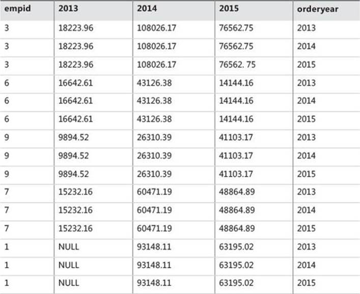
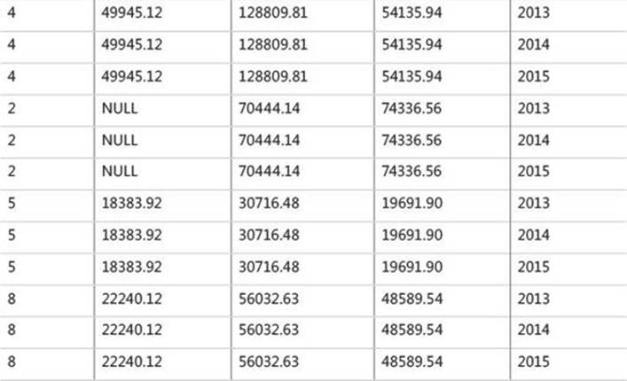
TABLE 1-10 Virtual table returned from UNPIVOT’s first step
The second step (U2) extracts the value from the source column corresponding to the unpivoted element that the current copy of the row represents. The name of the target column that will hold the values is specified right before the FOR clause (val in our case). The target column will contain the value from the source column corresponding to the current row’s order year from the virtual table. The virtual table returned from this step in our example is shown in Table 1-11.
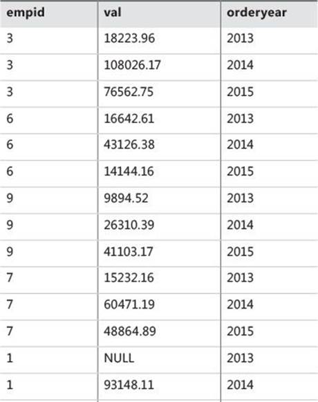
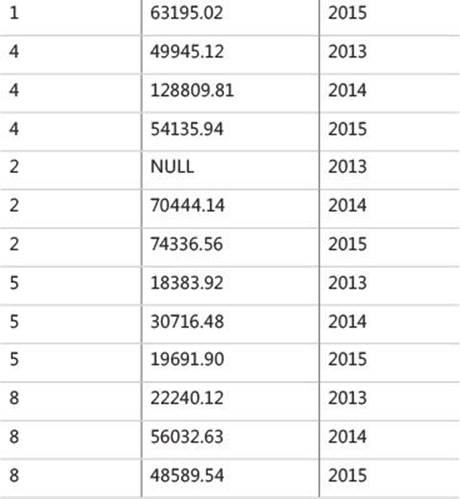
TABLE 1-11 Virtual table returned from UNPIVOT’s second step
UNPIVOT’s third and final step (U3) is to remove rows with NULLs in the result value column (val, in our case). The virtual table returned from this step in our example is shown in Table 1-12.
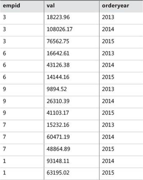
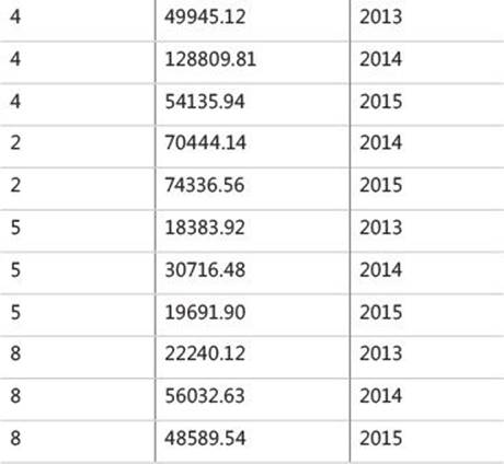
TABLE 1-12 Virtual table returned from UNPIVOT’s third step
When you’re done, run the following code for cleanup:
IF OBJECT_ID(N'dbo.EmpYearValues', N'U') IS NOT NULL DROP TABLE dbo.EmpYearValues;
Window functions
You use window functions to apply a data-analysis calculation against a set (a window) derived from the underlying query result set, per underlying row. You use a clause called OVER to define the window specification. T-SQL supports a number of types of window functions: aggregate, ranking, offset, and statistical. As is the practice with other features described in this chapter, the focus here will be just on the logical query-processing context.
As mentioned, the set that the window function applies to is derived from the underlying query result set. If you think about it in terms of logical query processing, the underlying query result set is achieved only when you get to the SELECT phase (5). Before this phase, the result is still shaping. For this reason, window functions are restricted only to the SELECT (5) and ORDER BY (6) phases, as Listing 1-3 highlights.
LISTING 1-3 Window functions in logical query processing
(5) SELECT (5-2) DISTINCT (7) TOP(<top_specification>) (5-1) <select_list>
(1) FROM (1-J) <left_table> <join_type> JOIN <right_table> ON <on_predicate>
| (1-A) <left_table> <apply_type> APPLY <right_input_table> AS <alias>
| (1-P) <left_table> PIVOT(<pivot_specification>) AS <alias>
| (1-U) <left_table> UNPIVOT(<unpivot_specification>) AS <alias>
(2) WHERE <where_predicate>
(3) GROUP BY <group_by_specification>
(4) HAVING <having_predicate>
(6) ORDER BY <order_by_list>
(7) OFFSET <offset_specification> ROWS FETCH NEXT <fetch_specification> ROWS ONLY;
Even though I didn’t really explain in detail yet how window functions work, I’d like to demonstrate their use in both phases where they are allowed. The following example includes the COUNT window aggregate function in the SELECT list:
USE TSQLV3;
SELECT orderid, custid,
COUNT(*) OVER(PARTITION BY custid) AS numordersforcust
FROM Sales.Orders
WHERE shipcountry = N'Spain';
This query produces the following output:
orderid custid numordersforcust
----------- ----------- ----------------
10326 8 3
10801 8 3
10970 8 3
10928 29 5
10568 29 5
10887 29 5
10366 29 5
10426 29 5
10550 30 10
10303 30 10
10888 30 10
10911 30 10
10629 30 10
10872 30 10
10874 30 10
10948 30 10
11009 30 10
11037 30 10
11013 69 5
10917 69 5
10306 69 5
10281 69 5
10282 69 5
Before any restrictions are applied, the starting set that the window function operates on is the virtual table provided to the SELECT phase as input—namely, VT4. The window partition clause restricts the rows from the starting set to only those that have the same custid value as in the current row. The COUNT(*) function counts the number of rows in that set. Remember that the virtual table that the SELECT phase operates on has already undergone WHERE filtering—that is, only orders shipped to Spain have been filtered.
You can also specify window functions in the ORDER BY list. For example, the following query sorts the rows according to the total number of output rows for the customer (in descending order):
SELECT orderid, custid,
COUNT(*) OVER(PARTITION BY custid) AS numordersforcust
FROM Sales.Orders
WHERE shipcountry = N'Spain'
ORDER BY COUNT(*) OVER(PARTITION BY custid) DESC;
This query generates the following output:
orderid custid numordersforcust
----------- ----------- ----------------
10550 30 10
10303 30 10
10888 30 10
10911 30 10
10629 30 10
10872 30 10
10874 30 10
10948 30 10
11009 30 10
11037 30 10
11013 69 5
10917 69 5
10306 69 5
10281 69 5
10282 69 5
10928 29 5
10568 29 5
10887 29 5
10366 29 5
10426 29 5
10326 8 3
10801 8 3
10970 8 3
The UNION, EXCEPT, and INTERSECT operators
This section focuses on the logical query-processing aspects of the operators UNION (both ALL and implied distinct versions), EXCEPT, and INTERSECT. These operators correspond to similar operators in mathematical set theory, but in SQL’s case are applied to relations, which are a special kind of a set. Listing 1-4 contains a general form of a query applying one of these operators, along with numbers assigned according to the order in which the different elements of the code are logically processed.
LISTING 1-4 General form of a query applying a UNION, EXCEPT, or INTERSECT operator
(1) query1
(2) <operator>
(1) query2
(3) [ORDER BY <order_by_list>]
The UNION, EXCEPT, and INTERSECT operators compare complete rows between the two inputs. There are two kinds of UNION operators supported in T-SQL. The UNION ALL operator returns one result set with all rows from both inputs combined. The UNION operator returns one result set with the distinct rows from both inputs combined (no duplicates). The EXCEPT operator returns distinct rows that appear in the first input but not in the second. The INTERSECT operator returns the distinct rows that appear in both inputs.
An ORDER BY clause is not allowed in the individual queries because the queries are supposed to return sets (unordered). You are allowed to specify an ORDER BY clause at the end of the query, and it will apply to the result of the operator.
In terms of logical processing, each input query is first processed separately with all its relevant phases (minus a presentation ORDER BY, which is not allowed). The operator is then applied, and if an ORDER BY clause is specified, it is applied to the result set.
Take the following query as an example:
USE TSQLV3;
SELECT region, city
FROM Sales.Customers
WHERE country = N'USA'
INTERSECT
SELECT region, city
FROM HR.Employees
WHERE country = N'USA'
ORDER BY region, city;
This query generates the following output:
region city
--------------- ---------------
WA Kirkland
WA Seattle
First, each input query is processed separately following all the relevant logical processing phases. The first query returns locations (region, city) of customers from the United States. The second query returns locations of employees from the United States. The INTERSECT operator returns distinct rows that appear in both inputs—in our case, locations that are both customer locations and employee locations. Finally, the ORDER BY clause sorts the rows by region and city.
As another example for logical processing phases, the following query uses the EXCEPT operator to return customers that have made no orders:
SELECT custid FROM Sales.Customers
EXCEPT
SELECT custid FROM Sales.Orders;
The first query returns the set of customer IDs from Customers, and the second query returns the set of customer IDs from Orders. The EXCEPT operator returns the set of rows from the first set that do not appear in the second set. Remember that a set has no duplicates; the EXCEPT operator returns distinct occurrences of rows from the first set that do not appear in the second set.
The result set’s column names are determined by the operator’s first input. Columns in corresponding positions must have compatible data types. Finally, when comparing rows, the UNION, EXCEPT, and INTERSECT operators implicitly use the distinct predicate. (One NULL is not distinct from another NULL; a NULL is distinct from a non-NULL value.)
Conclusion
Understanding logical query processing and the unique aspects of SQL is essential to SQL practitioners. By being familiar with those aspects of the language, you can produce correct solutions and explain your choices. Remember, the idea is to master the basics.