T-SQL Querying (2015)
Chapter 2. Query tuning
Chapter 1, “Logical query processing,” focused on the logical design of SQL. This chapter focuses on the physical implementation in the Microsoft SQL Server platform. Because SQL is based on a standard, you will find that the core language elements look the same in the different database platforms. However, because the physical layer is not based on a standard, there you will see bigger differences between the different platforms. Therefore, to be good at query tuning you need to get intimately familiar with the physical layer in the particular platform you are working with. This chapter covers various aspects of the physical layer in SQL Server to give you a foundation for query tuning.
To tune queries, you need to analyze query execution plans and look at performance measures that different performance tools give you. A critical step in this process is to try and identify which activities in the plan represent more work, and somehow connect the relevant parts of the performance measures to those activities. Once you have this part figured out, you need to try and eliminate or reduce the activities that represent the majority of the work.
To understand what you see in the query execution plans, you need to be very familiar with access methods. To understand access methods, well, you need to be very familiar with the internal data structures that SQL Server uses.
This chapter starts by covering internal data structures. It then describes tools you will use to measure query performance. Those topics are followed by a detailed discussion of access methods and an examination of query-execution plans involving those. This chapter also covers cardinality estimates, indexing features, prioritizing queries for tuning, index and query information and statistics, temporary tables, set-based versus iterative solutions, query tuning with query revisions, and parallel query execution.
This chapter focuses on the traditional disk-based tables. Memory-optimized tables are covered separately in Chapter 10, “In-Memory OLTP.”
Internals
This section focuses on internal data structures in SQL Server. It starts with a description of pages and extents. It then goes into a discussion about organizing tables as a heap versus as a B-tree and nonclustered indexes.
Pages and extents
A page is an 8-KB unit where SQL Server stores data. With disk-based tables, the page is the smallest I/O unit that SQL Server can read or write. Things change in this respect with memory-optimized tables, but as mentioned, those issues are discussed separately in Chapter 10. Figure 2-1shows an illustration of the page structure.
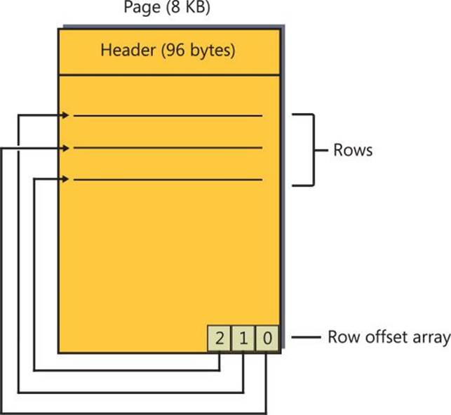
FIGURE 2-1 A diagram of a page.
The 96-byte header of the page holds information such as which allocation unit the page belongs to, pointers to the previous and next pages in the linked list in case the page is part of an index, the amount of free space in the page, and more. Based on the allocation unit, you can eventually figure out which object the page belongs to through the views sys.allocation_units and sys.partitions. For data and index pages, the body of the page contains the data or index records. At the end of the page, there’s the row-offset array, which is an array of two-byte pointers that point to the individual records in the page. The combination of the previous and next pointers in the page header and the row-offset array enforce index key order.
To work with a page for read or write purposes, SQL Server needs the page in the buffer pool (the data cache in memory). SQL Server cannot interact with a page directly in the data file on disk. If SQL Server needs to read a page and the page in question is already in the data cache as the result of some previous activity, it will perform only a logical read (read from memory). If the page is not already in memory, SQL Server will first perform a physical read, which pulls the page from the data file to memory, and then it will perform the logical read. Similarly, if SQL Server needs to write a page and the page is already in memory, it will perform a logical write. It will also set the dirty flag in the header of the page in memory to indicate that the state in memory is more recent than the state in the data file.
SQL Server periodically runs processes called lazywriter and checkpoint to write dirty pages from cache to disk, and it will sometimes use other threads to aid in this task. SQL Server uses an algorithm called LRU-K2 to prioritize which pages to free from the data cache based on the last two visits (recorded in the page header in memory). SQL Server uses mainly the lazywriter process to mark pages as free based on this algorithm.
An extent is a unit that contains eight contiguous pages, as shown in Figure 2-2.
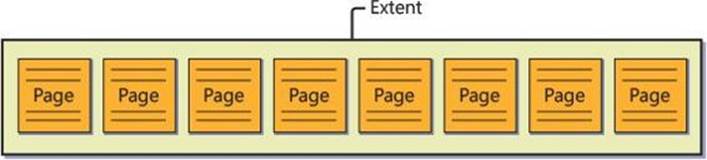
FIGURE 2-2 A diagram of an extent.
SQL Server supports two types of extents, called mixed and uniform. For new objects (tables or indexes), SQL Server allocates one page at a time from mixed extents until they reach a size of eight pages. So different pages of the same mixed extent can belong to different objects. SQL Server uses bitmap pages called shared global allocation maps (SGAMs) to keep track of which extents are mixed and have a page available for allocation. Once an object reaches a size of eight pages, SQL Server applies all future allocations of pages for it from uniform extents. A uniform extent is entirely owned by the same object. SQL Server uses bitmap pages called global allocation maps (GAMs) to keep track of which extents are free for allocation.
Table organization
A table can be organized in one of two ways—either as a heap or as a B-tree. Technically, the table is organized as a B-tree when it has a clustered index defined on it and as a heap when it doesn’t. You can create a clustered index directly using the CREATE CLUSTERED INDEX command or, starting with SQL Server 2014, using an inline clustered index definition INDEX <index_name> CLUSTERED. You can also create a clustered index indirectly through a primary key or unique constraint definition. When you add a primary-key constraint to a table, SQL Server will enforce it using a clustered index unless either you specify the NONCLUSTERED keyword explicitly or a clustered index already exists on the table. When you add a unique constraint to a table, SQL Server will enforce it using a nonclustered index unless you specify the CLUSTERED keyword. Either way, as mentioned, with a clustered index the table is organized as a B-tree and without one it is organized as a heap. Because a table must be organized in one of these two ways—heap or B-tree—the table organization is known as HOBT.
It’s far more common to see tables organized as B-trees in SQL Server. The main reason is probably that when you define a primary-key constraint, SQL Server enforces it with a clustered index by default. So, in cases where people create tables without thinking of the physical organization and define primary keys with their defaults, they end up with B-trees. As a result, there’s much more experience in SQL Server with B-trees than with heaps. Also, a clustered index gives a lot of control both on insertion patterns and on read patterns. For these reasons, with all other things being equal, I will generally prefer the B-tree organization by default.
There are cases where a heap can give you benefits. For example, in Chapter 6, “Data modification,” I describe bulk-import tools and the conditions you need to meet for the import to be processed with minimal logging. If the target table is a B-tree, it must be empty when you start the import if you want to get minimal logging. If it’s a heap, you can get minimal logging even if it already contains data. So, when the target table already contains some data and you’re adding a lot more, you can get better import performance if you first drop the indexes, do the import into a heap, and then re-create the indexes. In this example, you use a heap as a temporary state.
Regardless of how the table is organized, it can have zero or more nonclustered indexes defined on it. Nonclustered indexes are always organized as B-trees. The HOBT, as well as the nonclustered indexes, can be made of one or more units called partitions. Technically, the HOBT and each of the nonclustered indexes can be partitioned differently. Each partition of each HOBT and nonclustered index stores data in collections of pages known as allocation units. The three types of allocation units are known as IN_ROW_DATA, ROW_OVERFLOW_DATA, and LOB_DATA.
IN_ROW_DATA holds all fixed-length columns; it also holds variable-length columns as long as the row size does not exceed the 8,060-byte limit. ROW_OVERFLOW_DATA holds VARCHAR, NVARCHAR, VARBINARY, SQL_VARIANT, or CLR user-defined typed data that does not exceed 8,000 bytes but was moved from the original row because it exceeded the 8,060-row size limit. LOB_DATA holds large object values—VARCHAR(MAX), NVARCHAR(MAX), VARBINARY(MAX) that exceed 8,000 bytes, XML, or CLR UDTs. The system view sys.system_internals_allocation_units holds the anchors pointing to the page collections stored in the allocation units.
In the following sections, I describe the heap, clustered index, and nonclustered index structures. For simplicity’s sake, I’ll assume that the data is nonpartitioned; but if it is partitioned, the description is still applicable to a single partition.
Heap
A heap is a table that has no clustered index. The structure is called a heap because the data is not organized in any order; rather, it is laid out as a bunch of pages and extents. The Orders table in the sample database PerformanceV3 (see this book’s intro for details on how to install the sample database) is actually organized as a B-tree, but Figure 2-3 illustrates what it might look like when organized as a heap.
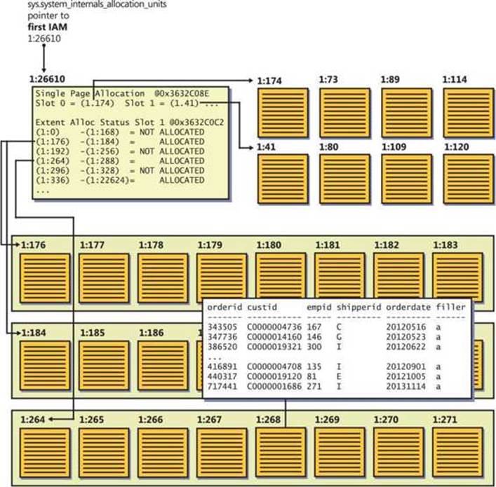
FIGURE 2-3 A diagram of a heap.
SQL Server maps the data that belongs to a heap using one or more bitmap pages called index allocation maps (IAMs). The header of the IAM page has pointers to the first eight pages that SQL Server allocated for the heap from mixed extents. The header also has a pointer to a starting location of a range of 4 GB that the IAM page maps in the data file. The body of the IAM page has a representative bit for each extent in that range. The bit is 0 if the extent it represents does not belong to the object owning the IAM page and 1 if it does. If one IAM is not enough to cover all the object’s data, SQL Server will maintain a chain of IAM pages. When SQL Server needs to scan a heap, it relies on the information in the IAM pages to figure out which pages and extents it needs to read. I will refer to this type of scan as an allocation order scan. This scan is done in file order and, therefore, when the data is not cached it usually applies sequential reads.
As you can see in Figure 2-3, SQL Server maintains internal pointers to the first IAM page and the first data page of a heap. Those pointers can be found in the system view sys.system_internals_allocation_units.
Because a heap doesn’t maintain the data in any particular order, new rows that are added to the table can go anywhere. SQL Server uses bitmap pages called page free space (PFS) to keep track of free space in pages so that it can quickly find a page with enough free space to accommodate a new row or allocate a new one if no such page exists.
When a row expands as a result of an update to a variable-length column and the page has no room for the row to expand, SQL Server moves the expanded row to a page with enough space to accommodate it and leaves behind what’s known as a forwarding pointer that points to the new location of the row. The purpose of forwarding pointers is to avoid the need to modify pointers to the row from nonclustered indexes when data rows move.
I didn’t yet explain a concept called a page split (because page splits can happen only in B-trees), but it suffices to say for now that heaps do not incur page splits.
B-tree (clustered index)
All indexes in SQL Server on disk-based tables are structured as B-trees, which are a special case of balanced trees. A balanced tree is a tree where no leaf is much farther away from the root than any other leaf.
A clustered index is structured as a B-tree, and it maintains the entire table’s data in its leaf level. The clustered index is not a copy of the data; rather, it is the data. Figure 2-4 illustrates how the Orders table might look when organized as a B-tree with the orderdate column defined as the key.
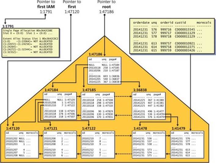
FIGURE 2-4 An illustration of a B-tree.
As you can see in the figure, the full data rows of the Orders table are stored in the index leaf level. The data rows are organized in the leaf in key order (orderdate in our case). A doubly linked list maintains the key order between the pages, and the row-offset array at the end of the page maintains this order within the page. When SQL Server needs to perform an ordered scan (or a range scan) operation in the leaf level of the index, it does so by following the linked list. I’ll refer to this type of scan as an index order scan.
Notice in Figure 2-4 that with each leaf row, the index maintains a column called uniquifier (abbreviated to unq in the illustration). The value in this column enumerates rows that have the same key value, and it is used together with the key value to uniquely identify rows when the index’s key columns are not unique. I’ll elaborate on the purpose of the uniquifier later when discussing nonclustered indexes.
When the optimizer optimizes a query, it needs to choose algorithms to handle operations such as joins, grouping and aggregating, distinct, window functions, and presentation order. Some operations can be processed only by using an order-based algorithm, like presentation order (ORDER BY clause in query). Some operations can be processed using more than one algorithm, including an order-based one. For example, grouping/aggregating and distinct can be processed either with an order-based algorithm or a hash-based one. Joins can be processed with an order-based algorithm, a hash-based algorithm, or a loop-based one. To use an order-based algorithm, the data needs to be arranged as ordered. One way for the optimizer to get the data ordered is to add an explicit sort operation to the plan. However, an explicit sort operation requires a memory grant and doesn’t scale well (N log N scaling).
Another way to get the data ordered is to perform an index order scan, assuming the right index exists. This option tends to be more efficient than the alternatives. Also, it doesn’t require a memory grant like explicit sort and hash operators do. When an index doesn’t exist, the optimizer is then left with just the remaining options. For operations that can be processed only with an order-based algorithm, like presentation order, the optimizer will have to add an explicit sort operation. For operations that can be processed with more than one algorithm, like grouping and aggregating, the optimizer will make a choice based on cost estimates. Because sorting doesn’t scale well, the optimizer tends to choose a strategy based on sorting with a small number of rows. Hash algorithms tend to scale better than sorting, so the optimizer tends to prefer hashing with a large number of rows.
Regarding the data in the leaf level of the index, the order of the pages in the file might not match the index key order. If page x points to next page y, and page y appears before page x in the file, page y is considered an out-of-order page. Logical scan fragmentation (also known asaverage fragmentation in percent) is measured as the percentage of out-of-order pages. So if there are 25,000 pages in the leaf level of the index and 5,000 of them are out of order, you have 20 percent of logical scan fragmentation. The main cause of logical scan fragmentation is page splits, which I’ll describe shortly. The higher the logical scan fragmentation of an index is, the slower an index order scan operation is when the data isn’t cached. This fragmentation tends to have little if any impact on index order scans when the data is cached.
Interestingly, in addition to the linked list, SQL Server also maintains IAM pages to map the data stored in the index in file order like it does in the heap organization. Recall that I referred to a scan of the data that is based on IAM pages as an allocation order scan. SQL Server might use this type of scan when it needs to perform unordered scans of the index’s leaf level. Because an allocation order scan reads the data in file order, its performance is unaffected by logical scan fragmentation, unlike with index order scans. Therefore, allocation order scans tend to be more efficient than index order scans, especially when the data isn’t cached and there’s a high level of logical scan fragmentation.
As mentioned, the main cause of logical scan fragmentation is page splits. A split of a leaf page occurs when a row needs to be inserted into the page and the target page does not have room to accommodate the row. Remember that an index maintains the data in key order. A row must enter a certain page based on its key value. If the target page is full, SQL Server will split the page. SQL Server supports two kinds of splits: one for an ascending key pattern and another for a nonascending key pattern.
If the new key is greater than or equal to the maximum key, SQL Server assumes that the insert pattern is an ascending key pattern. It allocates a new page and inserts the new row into that page. An ascending key pattern tends to be efficient when a single session adds new rows and the disk subsystem has a small number of drives. The new page is allocated in cache and filled with new rows. However, the ascending key pattern is not efficient when multiple sessions add new rows and your disk subsystem has many drives. With this pattern, there’s constant page-latch contention on the rightmost index page and insert performance tends to be suboptimal. An insert pattern with a random distribution of new keys tends to be much more efficient in such a scenario.
If the new key is less than the maximum key, SQL Server assumes that the insert pattern is a non-ascending key pattern. It allocates a new page, moves half the rows from the original page to the new one, and adjusts the linked list to reflect the right logical order of the pages. It inserts the new row either to the original page or to the new one based on its key value. The new page is not guaranteed to come right after the one that split—it could be somewhere later in the file, and it could also be somewhere earlier in the file.
Page splits are expensive, and they tend to result in logical scan fragmentation. You can measure the level of fragmentation in your index by querying the avg_fragmentation_in_percent attribute of the function sys.dm_db_index_physical_stats. To remove fragmentation, you rebuild the index using an ALTER INDEX REBUILD command. You can specify an option called FILLFACTOR with the percent that you want to fill leaf-level pages at the end of the rebuild. For example, using FILLFACTOR = 70 you request to fill leaf pages to 70 percent. With indexes that have a nonascending key insert pattern, it could be a good idea to leave some free space in the leaf pages to reduce occurrences of splits and to not let logical scan fragmentation evolve to high levels. You decide which fill factor value to use based on the rate of additions and frequency of rebuilds. With indexes that have an ascending key insert pattern, it’s pointless to leave empty space in the leaf pages because all new rows go to the right edge of the index anyway.
On top of the leaf level of the index, the index maintains additional levels, each summarizing the level below it. Each row in a nonleaf index page points to a whole page in the level below it, and together with the next row has information about the range of keys that the target page is responsible for. The row contains two elements: the minimum key column value in the index page being pointed to (assuming an ascending order) and a 6-byte pointer to that page. This way, you know that the target page is responsible for the range of keys that are greater than or equal to the key in the current row and less than the key in the next row. Note that in the row that points to the first page in the level below, the first element is NULL to indicate that there’s no minimum. As for the page pointer, it consists of the file number in the database and the page number in the file. When SQL Server builds an index, it starts from the leaf level and adds levels on top. It stops as soon as a level contains a single page, also known as the root page.
When SQL Server needs to find a certain key or range of keys at the leaf level of the index, it performs an access method called index seek. The access method starts by reading the root page and identifies the row that represents the range that contains the key being sought. It then navigates down the levels, reading one page in each level, until it reaches the page in the leaf level that contains the first matching key. The access method then performs a range scan in the leaf level to find all matching keys. Remember that all leaf pages are the same distance from the root. This means that the access method will read as many pages as the number of levels in the index to reach the first matching key. The I/O pattern of these reads is random I/O, as opposed to sequential I/O, because naturally the pages read by a seek operation until it reaches the leaf level will seldom reside next to each other.
In terms of our performance estimations, it is important to know the number of levels in an index because that number will be the cost of a seek operation in terms of page reads, and some execution plans invoke multiple seek operations repeatedly (for example, a Nested Loops join operator). For an existing index, you can get this number by invoking the INDEXPROPERTY function with the IndexDepth property. But for an index that you haven’t created yet, you need to be familiar with the calculations you can use to estimate the number of levels the index will contain.
The operands and steps required for calculating the number of levels in an index (call it L) are as follows (remember that these calculations apply to clustered and nonclustered indexes unless explicitly stated otherwise):
![]() The number of rows in the table (call it num_rows) This is 1,000,000 in our case.
The number of rows in the table (call it num_rows) This is 1,000,000 in our case.
![]() The average gross leaf row size (call it leaf_row_size) In a clustered index, this is actually the data row size. By “gross,” I mean that you need to take into consideration the internal overhead of the row and the 2-byte pointer in the row-offset array. The row overhead typically involves a few bytes. In our Orders table, the gross average data row size is roughly 200 bytes.
The average gross leaf row size (call it leaf_row_size) In a clustered index, this is actually the data row size. By “gross,” I mean that you need to take into consideration the internal overhead of the row and the 2-byte pointer in the row-offset array. The row overhead typically involves a few bytes. In our Orders table, the gross average data row size is roughly 200 bytes.
![]() The average leaf page density (call it page_density) This value is the average percentage of population of leaf pages. Page density is affected by things like data deletion, page splits, and rebuilding the index with a fillfactor value that is lower than 100. The clustered index in our table is based on an ascending key pattern; therefore, page_density in our case is likely going to be close to 100 percent.
The average leaf page density (call it page_density) This value is the average percentage of population of leaf pages. Page density is affected by things like data deletion, page splits, and rebuilding the index with a fillfactor value that is lower than 100. The clustered index in our table is based on an ascending key pattern; therefore, page_density in our case is likely going to be close to 100 percent.
![]() The number of rows that fit in a leaf page (call it rows_per_leaf_page) The formula to calculate this value is FLOOR((page_size – header_size) * page_density / leaf_row_size). In our case, rows_per_leaf_page amount to FLOOR((8192 – 96) * 1 / 200) = 40.
The number of rows that fit in a leaf page (call it rows_per_leaf_page) The formula to calculate this value is FLOOR((page_size – header_size) * page_density / leaf_row_size). In our case, rows_per_leaf_page amount to FLOOR((8192 – 96) * 1 / 200) = 40.
![]() The number of leaf pages (call it num_leaf_pages) This is a simple formula: num_rows / rows_per_leaf_page. In our case, it amounts to 1,000,000 / 40 = 25,000.
The number of leaf pages (call it num_leaf_pages) This is a simple formula: num_rows / rows_per_leaf_page. In our case, it amounts to 1,000,000 / 40 = 25,000.
![]() The average gross nonleaf row size (call it non_leaf_row_size) A nonleaf row contains the key columns of the index (in our case, only orderdate, which is 3 bytes); the 4-byte uniquifier (which exists only in a clustered index that is not unique); the page pointer, which is 6 bytes; a few additional bytes of internal overhead, which total 5 bytes in our case; and the row offset pointer at the end of the page, which is 2 bytes. In our case, the gross nonleaf row size is 20 bytes.
The average gross nonleaf row size (call it non_leaf_row_size) A nonleaf row contains the key columns of the index (in our case, only orderdate, which is 3 bytes); the 4-byte uniquifier (which exists only in a clustered index that is not unique); the page pointer, which is 6 bytes; a few additional bytes of internal overhead, which total 5 bytes in our case; and the row offset pointer at the end of the page, which is 2 bytes. In our case, the gross nonleaf row size is 20 bytes.
![]() The number of rows that fit in a nonleaf page (call it rows_per_non_leaf_page) The formula to calculate this value is similar to calculating rows_per_leaf_page. It’s FLOOR((page_size – header_size) / non_leaf_row_size), which in our case amounts to FLOOR((8192 – 96) / 20) = 404.
The number of rows that fit in a nonleaf page (call it rows_per_non_leaf_page) The formula to calculate this value is similar to calculating rows_per_leaf_page. It’s FLOOR((page_size – header_size) / non_leaf_row_size), which in our case amounts to FLOOR((8192 – 96) / 20) = 404.
![]() The number of levels above the leaf (call it L–1) This value is calculated with the following formula: CEILING(LOG(num_leaf_pages, rows_per_non_leaf_page)). In our case, L–1 amounts to CEILING(LOG(25000, 404)) = 2.
The number of levels above the leaf (call it L–1) This value is calculated with the following formula: CEILING(LOG(num_leaf_pages, rows_per_non_leaf_page)). In our case, L–1 amounts to CEILING(LOG(25000, 404)) = 2.
![]() The index depth (call it L) To get L you simply add 1 to L–1, which you computed in the previous step. The complete formula to compute L is CEILING(LOG(num_leaf_pages, rows_per_non_leaf_page)) + 1. In our case L amounts to 3.
The index depth (call it L) To get L you simply add 1 to L–1, which you computed in the previous step. The complete formula to compute L is CEILING(LOG(num_leaf_pages, rows_per_non_leaf_page)) + 1. In our case L amounts to 3.
![]() The number of rows that can be represented by an index with L levels (call it N) Suppose you are after the inverse computation of L. Namely, how many rows can be represented by an index with L levels. You compute rows_per_non_leaf_page and rows_per_leaf_page just like before. Then to compute N, use the formula: POWER(rows_per_non_leaf_page, L–1) * rows_per_leaf_page. For L = 3, rows_per_non_leaf_page = 404, and rows_per_leaf_page = 40, you get 6,528,540 rows.
The number of rows that can be represented by an index with L levels (call it N) Suppose you are after the inverse computation of L. Namely, how many rows can be represented by an index with L levels. You compute rows_per_non_leaf_page and rows_per_leaf_page just like before. Then to compute N, use the formula: POWER(rows_per_non_leaf_page, L–1) * rows_per_leaf_page. For L = 3, rows_per_non_leaf_page = 404, and rows_per_leaf_page = 40, you get 6,528,540 rows.
You can play with the preceding formulas for L and N and see that with up to about 16,000 rows, our index will have two levels. Three levels would support up to about 6,500,000 rows, and four levels would support up to about 2,600,000,000 rows. With nonclustered indexes, the formulas are the same—it’s just that you can fit more rows in each leaf page, as I will describe later. So with nonclustered indexes, the upper bound for each number of levels covers even more rows in the table. Our table has 1,000,000 rows, and all current indexes on our table have three levels. Therefore, the cost of a seek operation in any of the indexes on our table is three reads. Remember this number for later performance-related discussions in the chapter. As you can understand from this discussion, the number of levels in the index depends on the row size and the key size. But unless we’re talking about extreme sizes, as ballpark numbers you will probably get two levels with small tables (up to a few dozens of thousands of rows), three levels with medium tables (up to a few million rows), and four levels with large ones (up to a few billion rows).
Nonclustered index on a heap
A nonclustered index is also structured as a B-tree and in many respects is similar to a clustered index. The main difference is that a leaf row in a nonclustered index contains only the index key columns and a row locator value representing a particular data row. The content of the row locator depends on whether the underlying table is organized as a heap or as a B-tree. This section describes non-clustered indexes on a heap, and the following section will describe nonclustered indexes on a B-tree (clustered table).
Figure 2-5 illustrates the nonclustered index that SQL Server created to enforce our primary-key constraint (PK_Orders) with the orderid column as the key column. SQL Server assigned the index with the same name as the constraint, PK_Orders.
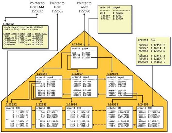
FIGURE 2-5 Nonclustered index on a heap.
The row locator used by a nonclustered index leaf row to point to a data row is an 8-byte physical pointer called a row identifier, or RID for short. It consists of the file number in the database, the target page number in the file, and the zero-based entry number in the row-offset array in the target page. When looking for a data row based on a given nonclustered index key, SQL Server first performs a seek operation in the index to find the leaf row with the key being sought. SQL Server then performs a RID lookup operation, which translates to reading the page that contains the data row, and then it pulls the row of interest from that page. Therefore, the cost of a RID lookup is one page read.
If you’re looking for a range of keys, SQL Server will perform a range scan in the index leaf and then a RID lookup per matching key. For a single lookup or a small number of lookups, the cost is not high, but for a large number of lookups, the cost can be very high because SQL Server ends up reading one whole page for each row being sought. For range queries that use a nonclustered index and a series of lookups—one per qualifying key—the cumulative cost of the lookup operations typically makes up the bulk of the cost of the query. I’ll demonstrate this point in the “Access methods” section. As for the cost of a seek operation, remember that the formulas I provided earlier for clustered indexes are just as relevant to nonclustered indexes. It’s just that the leaf_row_size is smaller, and therefore the rows_per_leaf_page will be higher. But the formulas are the same.
Nonclustered index on a B-tree
Nonclustered indexes created on a B-tree (clustered table) are architected differently than on a heap. The difference is that the row locator in a nonclustered index created on a B-tree is a value called a clustering key, as opposed to being a RID. The clustering key consists of the values of the clustered index keys from the row being pointed to and the uniquifier (if present). The idea is to point to a row logically as opposed to physically. This architecture was designed mainly for OLTP systems, where clustered indexes tend to incur frequent page splits upon data insertions and updates. If nonclustered indexes used RIDs as row locators, all pointers to the data rows that moved would have to be changed to reflect their new RIDs. Imagine the performance impact this would have with multiple nonclustered indexes defined on the table. Instead, SQL Server maintains logical pointers that don’t change when data rows move between leaf pages in the clustered index.
Figure 2-6 illustrates what the PK_Orders nonclustered index might look like; the index is defined with orderid as the key column, and the Orders table has a clustered index defined with orderdate as the key column.
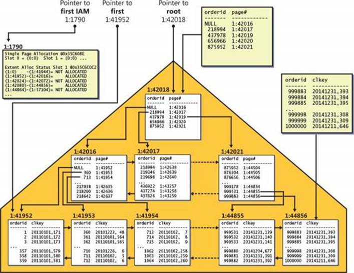
FIGURE 2-6 Nonclustered index on a B-tree.
A seek operation looking for a particular key in the nonclustered index (some orderid value) will end up reaching the relevant leaf row and have access to the row locator. The row locator in this case is the clustering key of the row being pointed to. To actually get to the row being pointed to, the lookup operation will need to perform a seek in the clustered index based on the acquired clustering key. This type of lookup is known as a key lookup, as opposed to a RID lookup. I will demonstrate this access method later in the chapter. The cost of each lookup operation (in terms of the number of page reads) is as high as the number of levels in the clustered index (3 in our case). That’s compared to a single page read for a RID lookup when the table is a heap. Of course, with range queries that use a nonclustered index and a series of lookups, the ratio between the number of logical reads in a heap case and a clustered table case will be close to 1:L, where L is the number of levels in the clustered index.
Tools to measure query performance
SQL Server gives you a number of tools to measure query performance, but one thing to keep in mind is that ultimately what matters is the user experience. The user mainly cares about two things: response time (the time it takes the first row to return) and throughput (the time it takes the query to complete). Naturally, as technical people we want to identify different performance measures that we believe are the major contributors to the eventual user experience. So we tend to look at things like number of reads (mainly interesting in I/O intensive activities), as well as CPU time and elapsed time.
The examples I will use in this chapter will be against a sample database called PerformanceV3. (See the book’s intro for details on how to install it.) Run the following code to connect to the sample database:
SET NOCOUNT ON;
USE PerformanceV3;
I will use the following query to demonstrate tools to measure query performance:
SELECT orderid, custid, empid, shipperid, orderdate, filler
FROM dbo.Orders
WHERE orderid <= 10000;
When you want to measure query performance in a test environment, you need to think about whether you expect the production environment to have hot or cold cache for the query. If the former, you want to execute the query twice and measure the performance of the second execution. The first execution will cause all pages to be brought into the data cache, and therefore the second execution will run against hot cache. If the latter, before you run your query, you want to run a manual checkpoint to write dirty buffers to disk and then drop all clean buffers from cache, like so:
CHECKPOINT;
DBCC DROPCLEANBUFFERS;
Note, though, that you should manually clear the data cache only in isolated test environments, because obviously this action will have a negative impact on the performance of queries. Both commands require elevated permissions.
I use three main, built-in tools to analyze and measure query performance: a graphical execution plan, the STATISTICS IO and STATISTICS TIME session options, and an Extended Events session with statement completed events. I use the graphical execution plan to analyze the plan that the optimizer created for the query. I use the session options when I need to measure the performance of a single query or a small number of queries. I use an Extended Events session when I need to measure the performance of a large number of queries.
Regarding the execution plan, you request to see the estimated plan in SQL Server Management Studio (SSMS) by highlighting your query and clicking the Display Estimated Execution Plan (Ctrl+L) button on the SQL Editor toolbar. You request to see the actual plan by enabling the Include Actual Execution Plan (Ctrl+M) button and executing the query. I generally prefer to analyze the actual plan because it includes run-time information like the actual number of rows returned by, and the actual number of executions of, each operator. Suboptimal choices made by the optimizer are often a result of inaccurate cardinality estimates, and those can be detected by comparing estimated and actual numbers in an actual execution plan.
Use the following code to enable measuring query performance with the session options STATISTICS IO (for I/O information) and STATISTICS TIME (for time information):
SET STATISTICS IO, TIME ON;
When you run a query, SSMS will report performance information in the Messages pane.
To measure the performance of ad hoc queries that you submit from SSMS using an Extended Events session, capture the event sql_statement_completed and filter the session ID of the SSMS session that you’re submitting the queries from. Use the following code to create and start such an Extended Events session after replacing the session ID with that of your SSMS session:
CREATE EVENT SESSION query_performance ON SERVER
ADD EVENT sqlserver.sql_statement_completed(
WHERE (sqlserver.session_id=(53))); -- replace with your session ID;
ALTER EVENT SESSION query_performance ON SERVER STATE = START;
To watch the event information, go to Object Explorer in SSMS. Navigate through the folder hierarchy Management\Extended Events\Sessions. Expand the Sessions folder, right-click the session query_performance, and choose Watch Live Data.
To show the output of the different performance-measuring tools, run the sample query after clearing the data cache. I got the actual query plan shown in Figure 2-7.
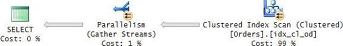
FIGURE 2-7 Execution plan for the sample query.
The plan is parallel. You can tell that an operator uses parallelism if it has a yellow circle with two arrows. The plan performs a parallel clustered index scan, which also applies a filter, and then it gathers the streams of rows returned by the different threads. An interesting point to note here is that the data flows in the plan from right to left as depicted by the direction of the arrows; however, the internal execution of the plan starts with the leftmost node, which is known as the root node. This node executes the node to its right requesting rows, and in turn that node executes the node to its right, requesting rows.
Following is the output generated by the STATISTICS IO option for this query:
Table 'Orders'. Scan count 9, logical reads 25339, physical reads 1, read-ahead reads 25138, lob
logical reads 0, lob physical reads 0, lob read-ahead reads 0.
The measure Scan count indicates how many times the object was accessed during the processing of the query. I think that the name of this measure is a bit misleading because any kind of access to the object adds to the count, not necessarily a scan. A name like Access count probably would have been more appropriate. In our case, the scan count is 9 because there were 8 threads that accessed the object in the parallel scan, plus a separate thread accessed the object for the serial parts of the plan.
The logical reads measure (25,339 in our case) indicates how many pages were read from the data cache. Note that if a page is read twice from cache, it is counted twice. Unfortunately, the STATISTICS IO tool does not indicate how many distinct pages were read. The measures physical reads (1 in our case) and read-ahead reads (25,138 in our case) indicate how many pages were read physically from disk into the data cache. As you can imagine, a physical read is much more expensive than a logical read. The physical reads measure represents a regular read mechanism. This mechanism uses synchronous reads of single-page units. By synchronous, I mean that the query processing cannot continue until the read is completed. The read-ahead reads measure represents a specialized read mechanism that anticipates the data that is needed for the query. This mechanism is referred to as read-ahead or prefetch. SQL Server usually uses this mechanism when a large-enough scan is involved. This mechanism applies asynchronous reads and might read chunks greater than a single page, all the way up to 512 KB per read. To help with troubleshooting, you can disable read-ahead by using trace flag 652. (Turn it on with DBCC TRACEON, and turn it off with DBCC TRACEOFF.) To find out the total number of physical reads that were involved in the processing of the query, sum the measures physical reads and read-ahead reads. In our case, the total is 25,139.
The STATISTICS IO output also shows logical reads, physical reads, and read-ahead reads for large object types separately. In our case, there are no large object types involved; therefore, all three measures are zeros.
The STATISTICS TIME option reports the following time statistics for our query:
SQL Server Execution Times:
CPU time = 170 ms, elapsed time = 765 ms.
Note that you will get multiple outputs from this option. In addition to getting the output for the execution of the query, you will also get output for the parsing and compilation of the query. You also will get outputs for every element you enable in SSMS that involves work that is submitted behind the scenes to SQL Server, like when you enable the graphical execution plan. The STATISTICS TIME output row that appears right after the STATISTICS IO output row is the one representing the query execution. To process our query against cold cache, SQL Server used 170 ms of CPU time and it took the query 765 ms of wall-clock time to complete.
Figure 2-8 shows the Watch Live Data window for the Extended Events session query_performance, with the execution of the sample query against cold cache highlighted.
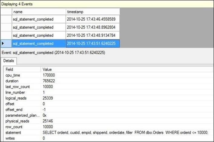
FIGURE 2-8 Information from the Extended Events session.
Now that the cache is hot, run the query a second time. I got the following output from STATISTICS IO:
Table 'Orders'. Scan count 9, logical reads 25339, physical reads 0, read-ahead reads 0, lob
logical reads 0, lob physical reads 0, lob read-ahead reads 0.
Notice that the measures representing physical reads are zeros. I got the following output from STATISTICS TIME:
CPU time = 265 ms, elapsed time = 299 ms.
Naturally, with hot cache the query finishes more quickly.
Access methods
This section provides a description of the various methods SQL Server uses to access data; it is designed to be used as a reference for discussions throughout this book involving the analysis of execution plans.
The examples in this section will use queries against the Orders table in the PerfromanceV3 database. This table is organized as a B-tree with the clustered index defined based on orderdate as the key. Use the following code to create a copy of the Orders table called Orders2, organized as a heap:
IF OBJECT_ID(N'dbo.Orders2', N'U') IS NOT NULL DROP TABLE dbo.Orders2;
SELECT * INTO dbo.Orders2 FROM dbo.Orders;
ALTER TABLE dbo.Orders2 ADD CONSTRAINT PK_Orders2 PRIMARY KEY NONCLUSTERED (orderid);
When I want to show access methods against a B-tree–organized table, I’ll query Orders. When I want to show access methods against a heap-organized table, I’ll query Orders2.
![]() Important
Important
I used randomization to generate the sample data in the PerformanceV3 database. This means that when you query objects in this database, your results probably will be slightly different than mine.
Most of the cost associated with access methods is related to I/O activity. Therefore, I’ll provide the number of logical reads as the main measure of the access methods’ performance.
Table scan/unordered clustered index scan
The first access method I’ll describe is a full scan of the table when there’s no requirement to return the data in any particular order. You get such a full scan in two main cases. One is when you really need all rows from the table. Another is when you need only a subset of the rows but don’t have a good index to support your filter. The tricky thing is that the query plan for such a full scan looks different depending on the underlying table’s organization (heap or B-tree). When the underlying table is a heap, the plan will show an operator called Table Scan. When the underlying table is a B-tree, the plan will show an operator called Clustered Index Scan with an Ordered: False property. I’ll refer to the former as a table scan and to the latter as an unordered clustered index scan.
A table scan or an unordered clustered index scan involves a scan of all data pages that belong to the table. The following query against the Orders2 table, which is structured as a heap, would require a table scan:
SELECT orderid, custid, empid, shipperid, orderdate, filler
FROM dbo.Orders2;
Figure 2-9 shows the graphical execution plan produced by the relational engine’s optimizer for this query, and Figure 2-10 shows an illustration of the way this access method is processed by the storage engine.
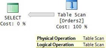
FIGURE 2-9 Heap scan (execution plan).
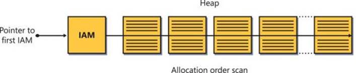
FIGURE 2-10 Heap scan (storage engine).
SQL Server reported 24,396 logical reads for this query on my system.
If you find it a bit confusing that both the Physical Operation and Logical Operation properties show Table Scan, you’re not alone. To me, the logical operation is a table scan and the physical operation is a heap scan.
The only option that the storage engine has to process a Table Scan operator is to use an allocation order scan. Recall from the section “Table organization” that an allocation order scan is performed based on IAM pages in file order.
The following query against the Orders table, which is structured as a B-tree, would require an unordered clustered index scan:
SELECT orderid, custid, empid, shipperid, orderdate, filler
FROM dbo.Orders;
Figure 2-11 shows the execution plan that the optimizer will produce for this query. Notice that the Ordered property of the Clustered Index Scan operator indicates False. Figure 2-12 shows an illustration of the two ways that the storage engine can carry out this access method.
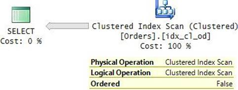
FIGURE 2-11 B-tree scan (execution plan).
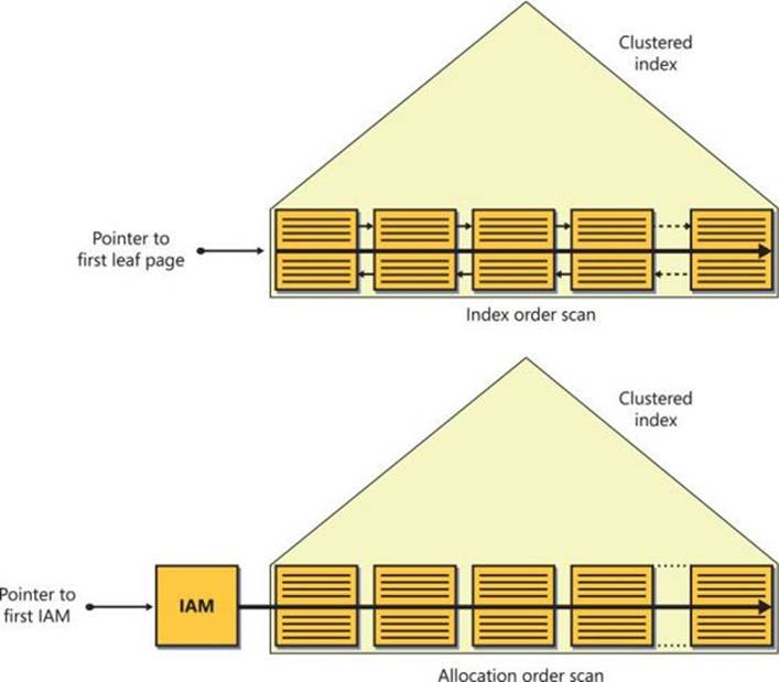
FIGURE 2-12 B-tree scan (storage engine).
SQL Server reported 25,073 logical reads for this query on my system.
Also, here I find it a bit confusing that the plan shows the same value in the Physical Operation and Logical Operation properties. This time, both properties show Clustered Index Scan. To me, the logical operation is still a table scan and the physical operation is a clustered index scan.
The fact that the Ordered property of the Clustered Index Scan operator indicates False means that as far as the relational engine is concerned, the data does not need to be returned from the operator in key order. This doesn’t mean that it is a problem if it is returned ordered; instead, it means that any order would be fine. This leaves the storage engine with some maneuvering space in the sense that it is free to choose between two types of scans: an index order scan (a scan of the leaf of the index following the linked list) and an allocation order scan (a scan based on IAM pages). The factors that the storage engine takes into consideration when choosing which type of scan to employ include performance and data consistency. I’ll provide more details about the storage engine’s decision-making process after I describe ordered index scans (Clustered Index Scan and Index Scan operators with the property Ordered: True).
Unordered covering nonclustered index scan
An unordered covering nonclustered index scan is similar to an unordered clustered index scan. The concept of a covering index means that a nonclustered index contains all columns specified in a query. In other words, a covering index is not an index with special properties; rather, it becomes a covering index with respect to a particular query. SQL Server can find all the data it needs to satisfy the query by accessing solely the index data, without needing to access the full data rows. Other than that, the access method is the same as an unordered clustered index scan, only, obviously, the leaf level of the covering nonclustered index contains fewer pages than the leaf of the clustered index because the row size is smaller and more rows fit in each page. I explained earlier how to calculate the number of pages in the leaf level of an index (clustered or nonclustered).
As an example of this access method, the following query requests all orderid values from the Orders table:
SELECT orderid
FROM dbo.Orders;
Our Orders table has a nonclustered index on the orderid column (PK_Orders), meaning that all the table’s order IDs reside in the index’s leaf level. The index covers our query. Figure 2-13 shows the graphical execution plan you would get for this query, and Figure 2-14 illustrates the two ways in which the storage engine can process it.
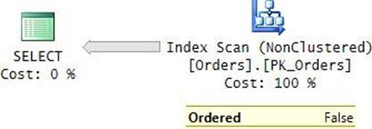
FIGURE 2-13 Unordered covering nonclustered index scan (execution plan).
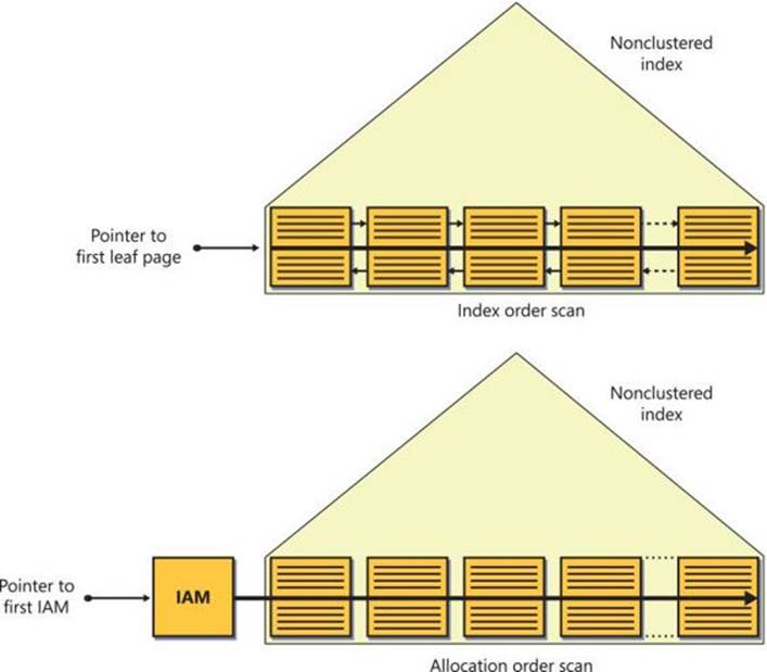
FIGURE 2-14 Unordered covering nonclustered index scan (storage engine).
SQL Server reported 2,611 logical reads for this query on my system. This is the number of pages making the leaf level of the PK_Orders index.
As a small puzzle for you, add the orderdate column to the query, like so:
SELECT orderid, orderdate
FROM dbo.Orders;
Examine the execution plan for this query as shown in Figure 2-15.
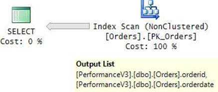
FIGURE 2-15 Index that includes a clustering key.
Observe that the PK_Orders index is still considered a covering one with respect to this query. The question is, how can this be the case when the index was defined explicitly only on the orderid column as the key? The answer is the table has a clustered index defined with the orderdatecolumn as the key. As you might recall, SQL Server uses the clustered index key as the row locator in nonclustered indexes. So, even though you defined the PK_Orders index explicitly only with the orderid column, SQL Server internally defined it with the columns orderid and orderdate. Never mind that SQL Server added the orderdate column to be used as the row locator—once it’s there, SQL Server can use it for other query-processing purposes.
Ordered clustered index scan
An ordered clustered index scan is a full scan of the leaf level of the clustered index that guarantees that the data will be returned to the next operator in index order. For example, the following query, which requests all orders sorted by orderdate, will get such an access method in its plan:
SELECT orderid, custid, empid, shipperid, orderdate, filler
FROM dbo.Orders
ORDER BY orderdate;
You can find the execution plan for this query in Figure 2-16 and an illustration of how the storage engine carries out this access method in Figure 2-17.
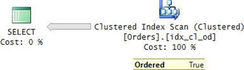
FIGURE 2-16 Ordered clustered index scan (execution plan).
FIGURE 2-17 Ordered clustered index scan (storage engine).
SQL Server reported 25,073 logical reads for this query on my system.
Notice in the plan that the Ordered property is True. This indicates that the data needs to be returned from the operator ordered. When the operator has the property Ordered: True, the scan can be carried out by the storage engine only in one way—by using an index order scan (a scan based on the index linked list), as shown in Figure 2-17. Unlike an allocation order scan, the performance of an index order scan depends on the fragmentation level of the index. With no fragmentation at all, the performance of an index order scan should be very close to the performance of an allocation order scan because both will end up reading the data in file order sequentially. However, with cold cache, as the fragmentation level grows, the performance difference will be more substantial—in favor of the allocation order scan, of course. The natural deductions are that you shouldn’t request the data sorted if you don’t need it sorted, to allow the potential for using an allocation order scan, and that you should resolve fragmentation issues in indexes that incur large index order scans against cold cache. I’ll elaborate on fragmentation and its treatment later.
Note that the optimizer is not limited to ordered-forward scans. Remember that the linked list is a doubly linked list, where each page contains both a next pointer and a previous pointer. Had you requested a descending sort order, you would have still gotten an ordered index scan, only ordered backward (from tail to head) instead of ordered forward (from head to tail). Interestingly, though, as of SQL Server 2014, the storage engine will consider using parallelism only with an ordered-forward scan. It always processes an ordered-backward scan serially.
SQL Server also supports descending indexes. One reason to use those is to enable parallel scans when parallelism is an important factor in the performance of the query. Another reason to use those is to support multiple key columns that have opposite directions in their sort requirements—for example, sorting by col1, col2 DESC. I’ll demonstrate using descending indexes later in the chapter in the section “Indexing features.”
Ordered covering nonclustered index scan
An ordered covering nonclustered index scan is similar to an ordered clustered index scan, with the former performing the access method in a nonclustered index—typically, when covering a query. The cost is, of course, lower than a clustered index scan because fewer pages are involved. For example, the PK_Orders index on our clustered Orders table covers the following query, and it has the data in the desired order:
SELECT orderid, orderdate
FROM dbo.Orders
ORDER BY orderid;
Figure 2-18 shows the query’s execution plan, and Figure 2-19 illustrates the way the storage engine processes the access method.
FIGURE 2-18 Ordered covering nonclustered index scan (execution plan).
FIGURE 2-19 Ordered covering nonclustered index scan (storage engine).
Notice in the plan that the Ordered property of the Index Scan operator shows True.
An ordered index scan is used not only when you explicitly request the data sorted, but also when the plan uses an operator that can benefit from sorted input data. This can be the case when processing GROUP BY, DISTINCT, joins, and other requests. This can also happen in less obvious cases. For example, check out the execution plan shown in Figure 2-20 for the following query:
SELECT orderid, custid, empid, orderdate
FROM dbo.Orders AS O1
WHERE orderid =
(SELECT MAX(orderid)
FROM dbo.Orders AS O2
WHERE O2.orderdate = O1.orderdate);
FIGURE 2-20 Ordered covering nonclustered index scan with segmentation.
The Segment operator arranges the data in groups and emits a group at a time to the next operator (Top in our case). Our query requests the orders with the maximum orderid per orderdate. Fortunately, we have a covering index for the task (idx_unc_od_oid_i_cid_eid), with the key columns being (orderdate, orderid) and included nonkey columns being (custid, empid). I’ll elaborate on included nonkey columns later in the chapter. The important point for our discussion is that the Segment operator organizes the data by groups of orderdate values and emits the data, a group at a time, where the last row in each group is the maximum orderid in the group; because orderid is the second key column right after orderdate. Therefore, the plan doesn’t need to sort the data; rather, the plan just collects it with an ordered scan from the covering index, which is already sorted by orderdate and orderid. The Top operator has a simple task of just collecting the last row (TOP 1 descending), which is the row of interest for the group. The number of rows reported by the Top operator is 1490, which is the number of unique groups (orderdate values), each of which got a single row from the operator. Because our nonclustered index covers the query by including in its leaf level all other columns that are mentioned in the query (custid, empid), there’s no need to look up the data rows; the query is satisfied by the index data alone.
The storage engine’s treatment of scans
Before I continue the coverage of additional access methods, I’m going to explain the way the storage engine treats the relational engine’s instructions to perform scans. The relational engine is like the brains of SQL Server; it includes the optimizer, which is in charge of producing execution plans for queries. The storage engine is like the muscles of SQL Server; it needs to carry out the instructions provided to it by the relational engine in the execution plan and perform the actual row operations. Sometimes the optimizer’s instructions leave the storage engine with some room for maneuvering, and then the storage engine determines the best of several possible options based on factors such as performance and consistency.
Allocation order scans vs. index order scans
When the plan shows a Table Scan operator, the storage engine has only one option: to use an allocation order scan. When the plan shows an Index Scan operator (clustered or nonclustered) with the property Ordered: True, the storage engine can use only an index order scan.
When the plan shows an Index Scan operator with Ordered: False, the relational engine doesn’t care in what order the rows are returned. In this case, there are two options to scan the data: allocation order scan and index order scan. It is up to the storage engine to determine which to employ. Unfortunately, the storage engine’s actual choice is not indicated in the execution plan, or anywhere else. I will explain the storage engine’s decision-making process, but it’s important to understand that what the plan shows is the relational engine’s instructions and not what the storage engine did.
The performance of an allocation order scan is not affected by logical fragmentation in the index because it’s done in file order, anyway. However, the performance of an index order scan that involves physical reads is affected by fragmentation—the higher the fragmentation, the slower the scan. Therefore, as far as performance is concerned, the storage engine considers the allocation order scan the preferable option. The exception is when the index is very small (up to 64 pages). In that case, the cost of interpreting IAM pages becomes significant with respect to the rest of the work, and the storage engine considers the index order scan to be preferable. Small tables aside, in terms of performance the allocation order scan is considered preferable.
However, performance is not the only aspect that the storage engine needs to take into consideration; it also needs to account for data-consistency expectations based on the effective isolation level. When there’s more than one option to carry out a request, the storage engine opts for the fastest option that meets the consistency requirements.
In certain circumstances, scans can end up returning multiple occurrences of rows or even skipping rows. Allocation order scans are more prone to such behavior than index order scans. I’ll first describe how such a phenomenon can happen with allocation order scans and in which circumstances. Then I’ll explain how it can happen with index order scans.
Allocation order scans
Figure 2-21 demonstrate in three steps how an allocation order scan can return multiple occurrences of rows.
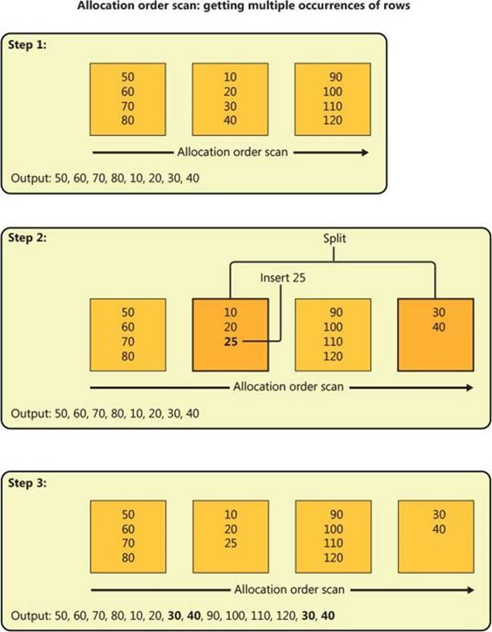
FIGURE 2-21 Allocation order scan: getting multiple occurrences of rows.
Step 1 shows an allocation order scan in progress, reading the leaf pages of some index in file order (not index order). Two pages were already read (keys 50, 60, 70, 80, 10, 20, 30, 40). At this point, before the third page of the index is read, someone inserts a row into the table with key 25.
Step 2 shows a split that took place in the page that was the target for the insert because it was full. As a result of the split, a new page was allocated—in our case, later in the file at a point that the scan did not yet reach. Half the rows from the original page move to the new page (keys 30, 40), and the new row with key 25 was added to the original page because of its key value.
Step 3 shows the continuation of the scan: reading the remaining two pages (keys 90, 100, 110, 120, 30, 40), including the one that was added because of the split. Notice that the rows with keys 30 and 40 were read a second time.
Of course, in a similar fashion, depending on how far the scan reaches by the time this split happens and where the new page is allocated, the scan might end up skipping rows. Figure 2-22 demonstrates how this can happen in three steps.
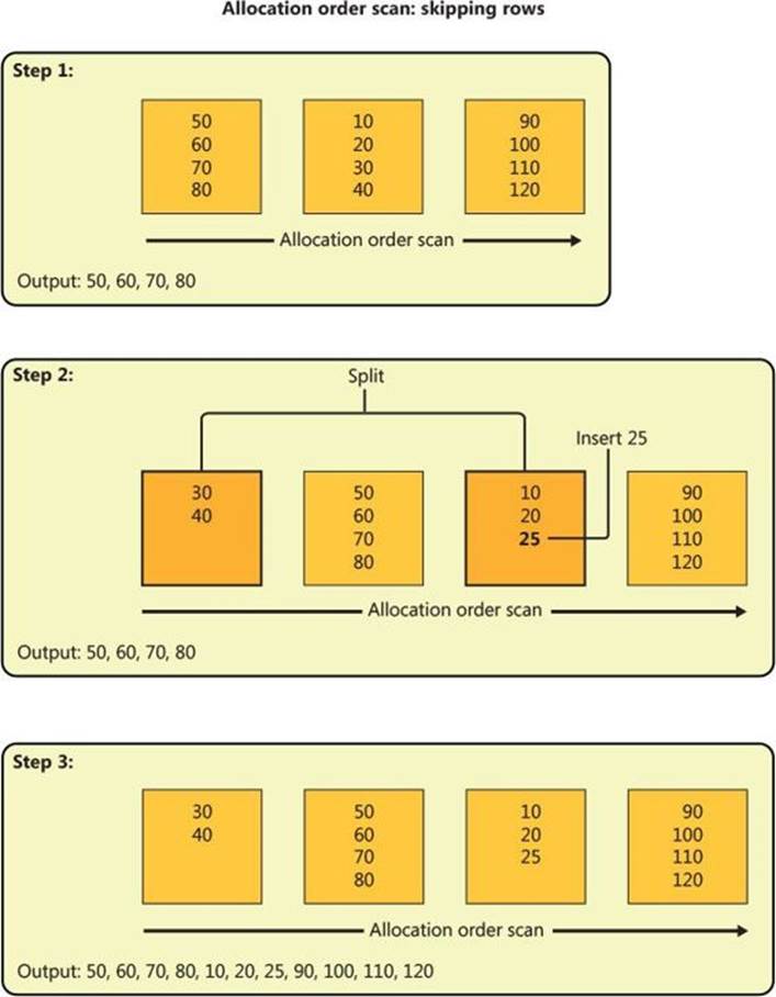
FIGURE 2-22 Allocation order scan: skipping rows.
Step 1 shows an allocation order scan in progress that manages to read one page (keys 50, 60, 70, 80) before the insert takes place.
Step 2 shows the split of the target page, only this time the new page is allocated earlier in the file at a point that the scan already passed. Like in the previous split example, the rows with keys 30 and 40 move to the new page, and the new row with key 25 is added to the original page.
Step 3 shows the continuation of the scan: reading the remaining two pages (keys 10, 20, 25, 90, 100, 110, 120). As you can see, the rows with keys 30 and 40 were completely skipped.
In short, an allocation order scan can return multiple occurrences of rows and skip rows resulting from splits that take place during the scan. A split can take place because of an insert of a new row, an update of an index key causing the row to move, or an update of a variable-length column causing the row to expand. Remember that splits take place only in indexes; heaps do not incur splits. Therefore, such phenomena cannot happen in heaps.
An index order scan is safer in the sense that it won’t read multiple occurrences of the same row or skip rows because of splits. Remember that an index order scan follows the index linked list in order. If a page that the scan hasn’t yet reached splits, the scan ends up reading both pages; therefore, it won’t skip rows. If a page that the scan already passed splits, the scan doesn’t read the new one; therefore, it won’t return multiple occurrences of rows.
The storage engine is well aware that allocation order scans are prone to such inconsistent reads because of splits, while index order scans aren’t. It will carry out an Index Scan Ordered: False with an allocation order scan in one of two categories of cases that I will refer to as the unsafeand safe categories.
The unsafe category is when the scan actually can return multiple occurrences of rows or skip rows because of splits. The storage engine opts for this option when the index size is greater than 64 pages and the request is running under the Read Uncommitted isolation level (for example, when you specify NOLOCK in the query). Most people’s perception of Read Uncommitted is simply that the query does not request a shared lock and therefore it can read uncommitted changes (dirty reads). This perception is true, but unfortunately most people don’t realize that to the storage engine, Read Uncommitted is also an indication that pretty much all bets are off in terms of consistency. In other words, it will opt for the faster option even at the cost of returning multiple occurrences of rows or skipping rows. When the query is running under the default Read Committed isolation level or higher, the storage engine will opt for an index order scan to prevent such phenomena from happening because of splits. To recap, the storage engine employs allocation order scans of the unsafe category when all the following conditions are true:
![]() The index size is greater than 64 pages.
The index size is greater than 64 pages.
![]() The plan shows Index Scan, Ordered: False.
The plan shows Index Scan, Ordered: False.
![]() The query is running under the Read Uncommitted isolation level.
The query is running under the Read Uncommitted isolation level.
![]() Changes are allowed to the data.
Changes are allowed to the data.
In terms of the safe category, the storage engine also opts for allocation order scans with higher isolation levels than Read Uncommitted when it knows that it is safe to do so without sacrificing the consistency of the read (at least as far as splits are concerned). For example, when you run the query using the TABLOCK hint, the storage engine knows that no one can change the data while the read is in progress. Therefore, it is safe to use an allocation order scan. Of course, this means that attempts by other sessions to modify the table will be blocked during the read. Another example where the storage engine knows that it is safe to employ an allocation order scan is when the index resides in a read-only filegroup or database. To summarize, the storage engine will use an allocation order scan of the safe category when the index size is greater than 64 pages and the data is read-only (because of the TABLOCK hint, read-only filegroup, or database).
Keep in mind that logical fragmentation has an impact on the performance of index order scans but not on that of allocation order scans. And based on the preceding information, you should realize that the storage engine will sometimes use index order scans to process an Index Scan operator with the Ordered: False property.
The next section will demonstrate both unsafe and safe allocation order scans.
Run the following code to create a table called T1:
SET NOCOUNT ON;
USE tempdb;
GO
-- Create table T1
IF OBJECT_ID(N'dbo.T1', N'U') IS NOT NULL DROP TABLE dbo.T1;
CREATE TABLE dbo.T1
(
clcol UNIQUEIDENTIFIER NOT NULL DEFAULT(NEWID()),
filler CHAR(2000) NOT NULL DEFAULT('a')
);
GO
CREATE UNIQUE CLUSTERED INDEX idx_clcol ON dbo.T1(clcol);
A unique clustered index is created on clcol, which will be populated with random GUIDs by the default expression NEWID(). Populating the clustered index key with random GUIDs should cause a large number of splits, which in turn should cause a high level of logical fragmentation in the index.
Run the following code to insert rows into the table using an infinite loop, and stop it after a few seconds (say 5, to allow more than 64 pages in the table):
SET NOCOUNT ON;
USE tempdb;
TRUNCATE TABLE dbo.T1;
WHILE 1 = 1
INSERT INTO dbo.T1 DEFAULT VALUES;
Run the following code to check the fragmentation level of the index:
SELECT avg_fragmentation_in_percent FROM sys.dm_db_index_physical_stats
(
DB_ID(N'tempdb'),
OBJECT_ID(N'dbo.T1'),
1,
NULL,
NULL
);
When I ran this code on my system, I got more than 99 percent fragmentation, which of course is very high. If you need more evidence to support the fact that the order of the pages in the linked list is different from their order in the file, you can use the undocumented DBCC IND command, which gives you the B-tree layout of the index:
DBCC IND(N'tempdb', N'dbo.T1', 0);
I prepared the following piece of code to spare you from having to browse through the output of DBCC IND in an attempt to figure out the index leaf layout:
CREATE TABLE #DBCCIND
(
PageFID INT,
PagePID INT,
IAMFID INT,
IAMPID INT,
ObjectID INT,
IndexID INT,
PartitionNumber INT,
PartitionID BIGINT,
iam_chain_type VARCHAR(100),
PageType INT,
IndexLevel INT,
NextPageFID INT,
NextPagePID INT,
PrevPageFID INT,
PrevPagePID INT
);
INSERT INTO #DBCCIND
EXEC (N'DBCC IND(N''tempdb'', N''dbo.T1'', 0)');
CREATE CLUSTERED INDEX idx_cl_prevpage ON #DBCCIND(PrevPageFID, PrevPagePID);
WITH LinkedList
AS
(
SELECT 1 AS RowNum, PageFID, PagePID
FROM #DBCCIND
WHERE IndexID = 1
AND IndexLevel = 0
AND PrevPageFID = 0
AND PrevPagePID = 0
UNION ALL
SELECT PrevLevel.RowNum + 1,
CurLevel.PageFID, CurLevel.PagePID
FROM LinkedList AS PrevLevel
JOIN #DBCCIND AS CurLevel
ON CurLevel.PrevPageFID = PrevLevel.PageFID
AND CurLevel.PrevPagePID = PrevLevel.PagePID
)
SELECT
CAST(PageFID AS VARCHAR(MAX)) + ':'
+ CAST(PagePID AS VARCHAR(MAX)) + ' ' AS [text()]
FROM LinkedList
ORDER BY RowNum
FOR XML PATH('')
OPTION (MAXRECURSION 0);
DROP TABLE #DBCCIND;
The code stores the output of DBCC IND in a temp table, then it uses a recursive query to follow the linked list from head to tail, and then it uses a technique based on the FOR XML PATH option to concatenate the addresses of the leaf pages into a single string in linked list order. I got the following output on my system:
1:132098 1:111372 1:133098 1:125591 1:137567 1:118198 1:128938 1:117929 1:136036 1:128595...
It’s easy to observe logical fragmentation here. For example, page 1:132098 points to the page 1:111372, which is earlier in the file.
Next, run the following code to query T1:
SELECT SUBSTRING(CAST(clcol AS BINARY(16)), 11, 6) AS segment1, *
FROM dbo.T1;
The last 6 bytes of a UNIQUEIDENTIFIER value represent the first segment that determines ordering; therefore, I extracted that segment with the SUBSTRING function so that it would be easy to see whether the rows are returned in index order. The execution plan of this query indicates a Clustered Index Scan, Ordered: False. However, because the environment is not read-only and the isolation level is the default Read Committed, the storage engine uses an index order scan. This query returns the rows in the output in index order. For example, here’s the output that I got on my system:
segment1 clcol filler
-------------- ------------------------------------ -------
0x0000ED83A06E F5F5CA72-48F6-4716-BBDC-0000ED83A06E a
0x0002672771DF 7B3D64FE-9197-487E-A354-0002672771DF a
0x0002EE4AF130 7D4A671D-5FBD-4B37-831C-0002EE4AF130 a
0x000395E30408 2A670CC5-5459-4506-9DCE-000395E30408 a
0x0004BD69D4ED 40CB1A42-48C7-4D9C-A5F4-0004BD69D4ED a
0x0005E14203C0 DCFFE73A-2125-490F-913B-0005E14203C0 a
0x00067DD63977 B49C5103-01E7-4745-B1C3-00067DD63977 a
0x0007B82DD187 1157F2E9-AD7E-4795-850F-0007B82DD187 a
0x0007BC012CC0 93ED4A5C-3AAD-4686-8CA1-0007BC012CC0 a
0x0007E73BEFB8 732072E7-A767-48A3-B2CF-0007E73BEFB8 a
...
Query the table again, this time with the NOLOCK hint:
SELECT SUBSTRING(CAST(clcol AS BINARY(16)), 11, 6) AS segment1, *
FROM dbo.T1 WITH (NOLOCK);
This time, the storage engine employs an allocation order scan of the unsafe category. Here’s the output I got from this code on my system:
segment1 clcol filler
-------------- ------------------------------------ -------
0x03D5CA43F8AE 7E1A28DE-B712-4F71-A553-03D5CA43F8AE a
0x426CDFD8DDB3 003EFE48-180E-4A8D-B6E1-426CDFD8DDB3 a
0x426D6A3FFC2C 9239BF31-1AA2-47F0-8B50-426D6A3FFC2C a
0x426E5C9673AD 2F0A49B8-2A7E-4C20-A22E-426E5C9673AD a
0x5EEBC295A84A 3743277C-0C72-48CF-A6B5-5EEBC295A84A a
0x97A52864E1D8 131BDF97-E015-42E2-B884-97A52864E1D8 a
0x78D967590D8C 7AA0F5BF-0BF1-4689-B851-78D967590D8C a
0x78DA17132327 F40CC88B-FC08-4534-842C-78DA17132327 a
0x78DACE8A159E 90BE7781-301F-48AB-A398-78DACE8A159E a
0x20C225A8A10D 547BD309-7804-4969-8A7F-20C225A8A10D a
...
Notice that this time the rows are not returned in index order. If splits occur while such a read is in progress, the read might end up returning multiple occurrences of rows and skipping rows.
As an example of an allocation order scan of the safe category, run the query with the TABLOCK hint:
SELECT SUBSTRING(CAST(clcol AS BINARY(16)), 11, 6) AS segment1, *
FROM dbo.T1 WITH (TABLOCK);
Here, even though the code is running under the Read Committed isolation level, the storage engine knows that it is safe to use an allocation order scan because no one can change the data during the read. I got the following output back from this query:
segment1 clcol filler
-------------- ------------------------------------ -------
0x03D5CA43F8AE 7E1A28DE-B712-4F71-A553-03D5CA43F8AE a
0x426CDFD8DDB3 003EFE48-180E-4A8D-B6E1-426CDFD8DDB3 a
0x426D6A3FFC2C 9239BF31-1AA2-47F0-8B50-426D6A3FFC2C a
0x426E5C9673AD 2F0A49B8-2A7E-4C20-A22E-426E5C9673AD a
0x5EEBC295A84A 3743277C-0C72-48CF-A6B5-5EEBC295A84A a
0x97A52864E1D8 131BDF97-E015-42E2-B884-97A52864E1D8 a
0x78D967590D8C 7AA0F5BF-0BF1-4689-B851-78D967590D8C a
0x78DA17132327 F40CC88B-FC08-4534-842C-78DA17132327 a
0x78DACE8A159E 90BE7781-301F-48AB-A398-78DACE8A159E a
0x20C225A8A10D 547BD309-7804-4969-8A7F-20C225A8A10D a
...
Next I’ll demonstrate how an unsafe allocation order scan can return multiple occurrences of rows. Open two connections (call them connection 1 and connection 2). Run the following code in connection 1 to insert rows into T1 in an infinite loop, causing frequent splits:
SET NOCOUNT ON;
USE tempdb;
TRUNCATE TABLE dbo.T1;
WHILE 1 = 1
INSERT INTO dbo.T1 DEFAULT VALUES;
Run the following code in connection 2 to read the data in a loop while connection 1 is inserting data:
SET NOCOUNT ON;
USE tempdb;
WHILE 1 = 1
BEGIN
SELECT * INTO #T1 FROM dbo.T1 WITH(NOLOCK);
IF EXISTS(
SELECT clcol
FROM #T1
GROUP BY clcol
HAVING COUNT(*) > 1) BREAK;
DROP TABLE #T1;
END
SELECT clcol, COUNT(*) AS cnt
FROM #T1
GROUP BY clcol
HAVING COUNT(*) > 1;
DROP TABLE #T1;
The SELECT statement uses the NOLOCK hint, and the plan shows Clustered Index Scan, Ordered: False, meaning that the storage engine will likely use an allocation order scan of the unsafe category. The SELECT INTO statement stores the output in a temporary table so that it will be easy to prove that rows were read multiple times. In each iteration of the loop, after reading the data into the temp table, the code checks for multiple occurrences of the same GUID in the temp table. This can happen only if the same row was read more than once. If duplicates are found, the code breaks from the loop and returns the GUIDs that appear more than once in the temp table. When I ran this code, after a few seconds I got the following output in connection 2 showing all the GUIDs that were read more than once:
clcol cnt
------------------------------------ -----------
F144911F-44B8-4AC7-9396-D2C26DBB9E2E 2
990B829E-739D-4AA1-BD59-F55DFF8E9530 2
9A02C46B-389E-45A1-AC07-90DB4115D43B 2
B5BAF81C-B2B5-492A-9E9A-DB566E4A5A98 2
132255C8-63F5-4DB7-9126-D37C1F321868 2
69A77E96-B748-48A8-94A2-85B6A270F5D1 2
7F3C7E7A-8181-44BB-8D0F-0F39AA001DC2 2
B5C5C70D-B721-4225-8455-F56910DA2CD1 2
9E2588DA-CB57-4CA0-A10D-F08B0306B6A6 2
F50AA680-E754-4B61-8335-F08A3C965924 2
...
At this point, you can stop the code in connection 1.
If you want, you can rerun the test without the NOLOCK hint and see that the code in connection 2 doesn’t stop, because duplicate GUIDs are not found.
Next I’ll demonstrate an unsafe allocation order scan that skips rows. Run the following code to create the tables T1 and MySequence:
-- Create table T1
SET NOCOUNT ON;
USE tempdb;
IF OBJECT_ID(N'dbo.T1', N'U') IS NOT NULL DROP TABLE dbo.T1;
CREATE TABLE dbo.T1
(
clcol UNIQUEIDENTIFIER NOT NULL DEFAULT(NEWID()),
seqval INT NOT NULL,
filler CHAR(2000) NOT NULL DEFAULT('a')
);
CREATE UNIQUE CLUSTERED INDEX idx_clcol ON dbo.T1(clcol);
-- Create table MySequence
IF OBJECT_ID(N'dbo.MySequence', N'U') IS NOT NULL DROP TABLE dbo.MySequence;
CREATE TABLE dbo.MySequence(val INT NOT NULL);
INSERT INTO dbo.MySequence(val) VALUES(0);
The table T1 is similar to the one used in the previous demonstration, but this one has an additional column called seqval that will be populated with sequential integers. The table MySequence holds the last-used sequence value (populated initially with 0), which will be incremented by 1 before each insert to T1. To prove that a scan skipped rows, you simply need to show that the output of the scan has gaps between contiguous values in the seqval column. I’m not using the built-in sequence object in my test because SQL Server doesn’t guarantee that you won’t have gaps between sequence values, regardless of the cache setting you use. To demonstrate this behavior, open two connections (again, call them connection 1 and connection 2). Run the following code from connection 1 to insert rows into T1 in an infinite loop, and increment the sequence value by 1 in each iteration:
SET NOCOUNT ON;
USE tempdb;
UPDATE dbo.MySequence SET val = 0;
TRUNCATE TABLE dbo.T1;
DECLARE @nextval AS INT;
WHILE 1 = 1
BEGIN
UPDATE dbo.MySequence SET @nextval = val += 1;
INSERT INTO dbo.T1(seqval) VALUES(@nextval);
END
Run the following code in connection 2 while the inserts are running in connection 1:
SET NOCOUNT ON;
USE tempdb;
DECLARE @max AS INT;
WHILE 1 = 1
BEGIN
SET @max = (SELECT MAX(seqval) FROM dbo.T1);
SELECT * INTO #T1 FROM dbo.T1 WITH(NOLOCK);
CREATE NONCLUSTERED INDEX idx_seqval ON #T1(seqval);
IF EXISTS(
SELECT *
FROM (SELECT seqval AS cur,
(SELECT MIN(seqval)
FROM #T1 AS N
WHERE N.seqval > C.seqval) AS nxt
FROM #T1 AS C
WHERE seqval <= @max) AS D
WHERE nxt - cur > 1) BREAK;
DROP TABLE #T1;
END
SELECT *
FROM (SELECT seqval AS cur,
(SELECT MIN(seqval)
FROM #T1 AS N
WHERE N.seqval > C.seqval) AS nxt
FROM #T1 AS C
WHERE seqval <= @max) AS D
WHERE nxt - cur > 1;
DROP TABLE #T1;
This code runs an infinite loop that in each iteration reads the data using NOLOCK into a temp table and breaks from the loop as soon as contiguous values with a gap between them are found in the seqval column. The code then presents the pairs of contiguous values that have a gap between them. After a few seconds, I got the following output in connection 2, shown here in abbreviated form:
cur nxt
----------- -----------
8128 8130
12378 12380
13502 13504
17901 17903
25257 25259
27515 27517
29782 29784
32764 32766
32945 32947
...
You can stop the code in connection 1.
You can run the test again without the NOLOCK hint, in which case the storage engine will use an index order scan. The code in connection 2 should not break from the loop, because gaps won’t be found.
Index order scans
If you think that index order scans are safe from phenomena such as returning multiple occurrences of rows or skipping rows, think again. It is true that index order scans are safe from such phenomena because of page splits, but page splits are not the only reason for data to move around in the index leaf.
Another cause of movement in the leaf is update of an index key. If an index key is modified after the row was read by an index order scan and the row is moved to a point in the leaf that the scan hasn’t reached yet, the scan will read the row a second time. Similarly, if an index key is modified before the row is read by an index order scan and the row is moved to a point in the leaf that the scan has already passed, the scan will never reach that row.
For example, suppose you have an Employees table that currently has four employee rows (employee A with a salary of 2000, employee B with a salary of 4000, employee C with a salary of 3000, and employee D with a salary of 1000). A clustered index is defined on the salary column as the key. Figure 2-23 shows in three steps how an index order scan can return multiple occurrences of the same row because of an update that takes place during the read.
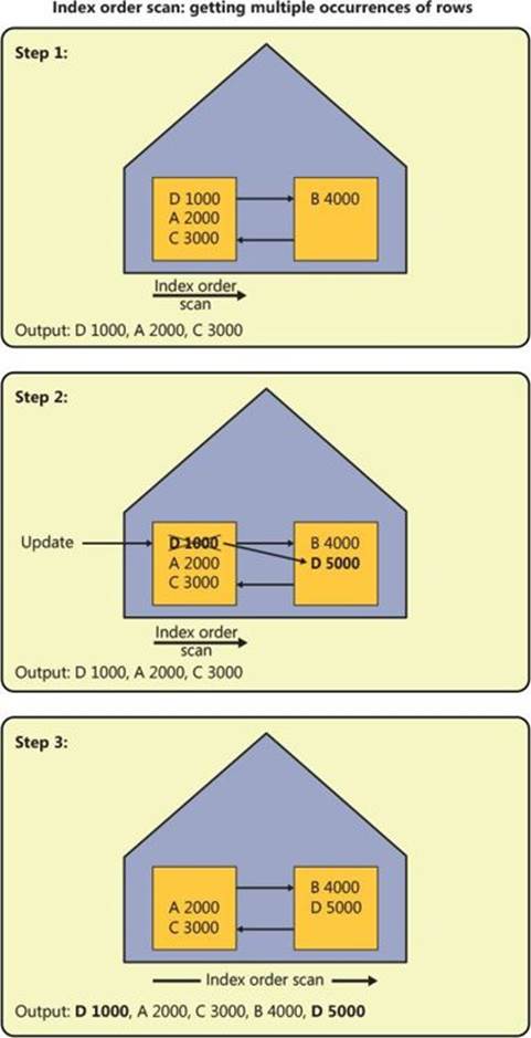
FIGURE 2-23 Index order scan: getting multiple occurrences of rows.
You issue a query against the table, and the storage engine uses an index order scan. Remember that an index order scan is always used when the plan shows Index Scan: Ordered: True (for example, when the query has an ORDER BY clause), but it also does so when the Ordered property is False, the environment is read/write, and the isolation level is not Read Uncommitted.
Step 1 shows that the scan already read the first page in the leaf level and returned the rows for employees D, A, and C. If the query is running under Read Uncommitted, no shared locks are acquired on the rows. If the query is running under Read Committed, shared locks are acquired, but they are released as soon as the query is done with the resource (for example, a row or page), even though the query hasn’t finished yet. This means that at the point in time that the scan is done with the page, under both isolation levels no locks are held on the rows that were read.
Step 2 shows an update of the row for employee D, increasing the salary from 1000 to 5000. The row moves to the second page in the leaf level because of the index key change.
Step 3 shows the continuation of the scan, reading the second page in the leaf of the index, and returning the rows for employees B and D. Note that employee D was returned a second time. The first time, the row was returned with salary 1000 and the second time with salary 5000. Note that this phenomenon cannot happen under higher isolation levels than Read Committed because those isolation levels keep shared locks until the end of the transaction. This phenomenon also cannot happen under the two isolation levels that are based on row versioning: Read Committed Snapshot and Snapshot.
Similarly, an index order scan can skip rows. Figure 2-24 shows how this can happen in three steps.
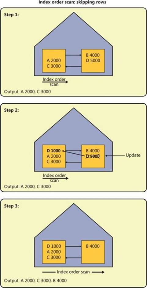
FIGURE 2-24 Index order scan: skipping rows.
Employee D starts with salary 5000 this time, and its row resides in the second index leaf page. Step 1 shows that the scan already read the first page in the leaf level and returned the rows for employees A and C.
Step 2 shows an update of the row for employee D, decreasing the salary from 5000 to 1000. The row moves to the first page in the leaf level because of the index key change.
Step 3 shows the continuation of the scan, reading the second page in the leaf of the index, returning the rows for employee B. Note that the row for employee D was not returned at all—neither with the salary 5000 nor with 1000. Note that this phenomenon can happen in Read Uncommitted, Read Committed, and even Repeatable Read because the update was done to a row that was not yet read. This phenomenon cannot happen under the isolation levels Serializable, Read Committed Snapshot, and Snapshot.
To see both phenomena for yourself, you can run a simple test. First, execute the following code to create and populate the Employees table:
SET NOCOUNT ON;
USE tempdb;
IF OBJECT_ID(N'dbo.Employees', N'U') IS NOT NULL DROP TABLE dbo.Employees;
CREATE TABLE dbo.Employees
(
empid VARCHAR(10) NOT NULL,
salary MONEY NOT NULL,
filler CHAR(2500) NOT NULL DEFAULT('a')
);
CREATE CLUSTERED INDEX idx_cl_salary ON dbo.Employees(salary);
ALTER TABLE dbo.Employees
ADD CONSTRAINT PK_Employees PRIMARY KEY NONCLUSTERED(empid);
INSERT INTO dbo.Employees(empid, salary) VALUES
('D', 1000.00),('A', 2000.00),('C', 3000.00),('B', 4000.00);
Open two connections. Run the following code in connection 1 to run an infinite loop that in each iteration updates the salary of employee D from its current value to 6000 minus its current value (switching between the values 1000 and 5000):
SET NOCOUNT ON;
USE tempdb;
WHILE 1=1
UPDATE dbo.Employees
SET salary = 6000.00 - salary
WHERE empid = 'D';
This code causes the row for employee D to keep moving between the two index leaf pages. Run the following code in connection 2:
SET NOCOUNT ON;
USE tempdb;
WHILE 1 = 1
BEGIN
SELECT * INTO #Employees FROM dbo.Employees;
IF @@rowcount <> 4 BREAK; -- use < 4 for skipping, > 4 for multi occur
DROP TABLE #Employees;
END
SELECT * FROM #Employees;
DROP TABLE #Employees;
The code runs an infinite loop that reads the contents of the Employees table into a temp table. Because the code doesn’t specify the NOLOCK hint and the environment is read/write, the storage engine uses an index order scan. The code breaks from the loop when the number of rows read is different than the expected number (four). In cases where the scan reads the same row twice, this code returns five rows in the output:
empid salary filler
---------- --------------------- ------
D 1000.00 a
A 2000.00 a
C 3000.00 a
B 4000.00 a
D 5000.00 a
In cases where the scan skips a row, this code returns three rows in the output:
empid salary filler
---------- --------------------- ------
A 2000.00 a
C 3000.00 a
B 4000.00 a
You can change the filter to < 4 to wait for a case where the row is skipped, and you can change it to > 4 to wait for a case where the row is read twice.
I hope this section gave you a better understanding of how the storage engine handles scans and, most importantly, the implications of running your code under the Read Uncommitted isolation level. The next sections continue the coverage of access methods.
Nonclustered index seek + range scan + lookups
The access method nonclustered index seek + range scan + lookups is typically used for small-range queries (including a point query) using a nonclustered index that doesn’t cover the query. For example, suppose you want to query orders with an order ID that falls within a small range of order IDs, like orderid <= 25. For qualifying orders, you want to return the columns orderid, custid, empid, shipperid, orderdate, and filler. We do have a nonclustered noncovering index called PK_Orders, which is defined with the orderid column as the key. The index can support the filter; however, because the index doesn’t cover the query, lookups will be required to obtain the remaining columns from the respective data rows. If the target table is a heap, the lookups will be RID lookups, each costing one page read. If the underlying table is a B-tree, the lookups will be key lookups, each costing as many reads as the number of levels in the clustered index.
To demonstrate this access method against a heap, I will use the following query:
USE PerformanceV3;
SELECT orderid, custid, empid, shipperid, orderdate, filler
FROM dbo.Orders2
WHERE orderid <= 25;
Figure 2-25 shows the query’s execution plan, and Figure 2-26 illustrates the way the storage engine processes the access method.
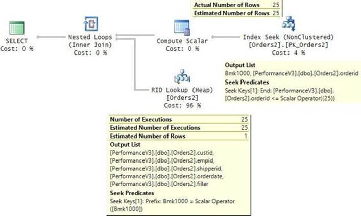
FIGURE 2-25 Nonclustered index seek + range scan + lookups against a heap (execution plan).
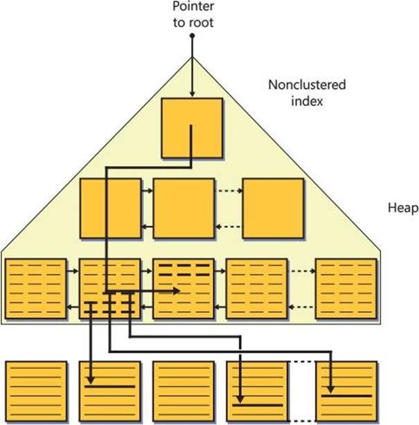
FIGURE 2-26 Nonclustered index seek + range scan + lookups against a heap (storage engine).
At the top right of the plan, the Index Seek operator against the PK_Orders2 index performs a seek in the index to the first matching row, and then it performs a range scan to identify all qualifying rows (25 in our case). The purpose of this activity is to collect the row locators (RIDs in the heap case) of the target data rows. The seek costs three reads. As for the cost of the range scan, it depends on how many qualifying rows there are and how many fit in a leaf page. This index can fit close to 400 rows per leaf page. So, in our case, the 25 qualifying rows probably reside in the first page in the leaf that the seek operation reached. So it’s very likely no additional page reads will be required for the range scan. The third part of the access method is to apply lookups based on the returned row locators to collect the remaining columns from the respective data rows. The lookups are activated by the Nested Loops operator per row that is returned from the Index Seek operator. Because this example involves a heap, the lookups are RID lookups, each costing one page read. With 25 qualifying rows, the lookups cost 25 reads in total. All in all, the total number of reads our query performs is 3 + 0 + 25 = 28. That’s exactly the number of reads that SQL Server reported for this query on my system.
To demonstrate this access method against a B-tree, I will use the following query:
SELECT orderid, custid, empid, shipperid, orderdate, filler
FROM dbo.Orders
WHERE orderid <= 25;
Figure 2-27 shows the query’s execution plan, and Figure 2-28 illustrates the way the storage engine processes the access method.
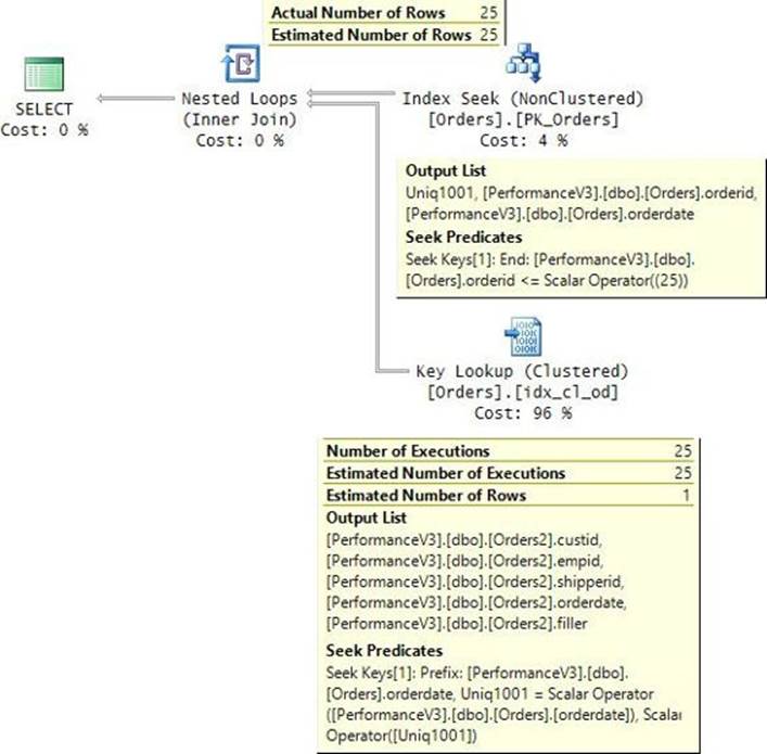
FIGURE 2-27 Nonclustered index seek + range scan + lookups against a B-tree (execution plan).
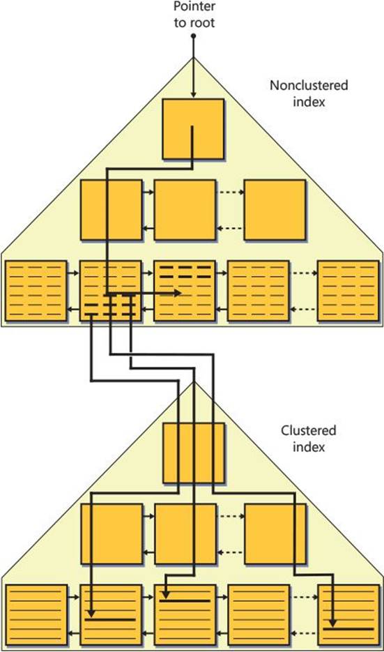
FIGURE 2-28 Nonclustered index seek + range scan + lookups against a B-tree (storage engine).
The key difference in this access method compared to the previous one is that instead of applying RID lookups, it applies key lookups. Remember that a key lookup translates to a seek in the clustered index and costs as many reads as the number of levels in the clustered index (3 in our case). So the total number of reads that our query performs is 3 + 0 + 25 * 3 = 78. That’s exactly the number of reads that SQL Server reported for this query on my system.
Now that the fundamental aspects of this access method have been covered, we can move on to some more interesting aspects, like cardinality estimates, prefetch, and tipping points.
When optimizing a query like the one in our example, the optimizer needs to make a number of choices that depend on the estimated cardinality of the filter (the estimated number of rows returned). Before I describe the specific choices the optimizer needs to make here, I’ll first describe the cardinality estimation method that it uses for this query. Generally, making cardinality estimates is quite a tricky business, as I will elaborate on later in this chapter in the section “Cardinality estimates.” Our particular case is pretty straightforward, though.
When you create an index, SQL Server also creates statistics about the data in the index. The statistics include a header with general information, density information about vectors of leading key columns in the index, and a histogram on the leading key column in the index. The histogram represents the distribution of key values within the column. Run the following code to show the histogram that SQL Server created based on the orderid column as part of the statistics for the PK_Orders index on the Orders table:
DBCC SHOW_STATISTICS (N'dbo.Orders', N'PK_Orders') WITH HISTOGRAM;
This code generated the following output on my system:
RANGE_HI_KEY RANGE_ROWS EQ_ROWS DISTINCT_RANGE_ROWS AVG_RANGE_ROWS
------------ ------------- ------------- -------------------- --------------
1 0 1 0 1
1000000 999998 1 999998 1
SQL Server supports histograms with up to 200 steps. But in our case, because the table has a consecutive range of order IDs between 1 and 1,000,000, SQL Server figured that it can adequately represent such data distribution with only two steps. Each step represents the keys greater than the previous step’s RANGE_HI_KEY value and less than or equal to the current step’s RANGE_HI_KEY value. The EQ_ROWS value represents how many rows have a key value equal to the RANGE_HI_KEY value. The RANGE_ROWS value indicates how many rows have a value greater than the previous step’s RANGE_HI_KEY value and less than (but not equal to) the current step’s RANGE_HI_KEY value. Similarly, the DISTINCT_RANGE_ROWS value indicates how many distinct values are greater than the previous step’s RANGE_HI_KEY value and less than the current step’s RANGE_HI_KEY value. The AVG_RANGE_ROWS value indicates the average number of rows per distinct value in the step.
You can see in Figure 2-27 (and the same in Figure 2-25) that the optimizer made an accurate cardinality estimate for our query filter based on this histogram. The estimated number of rows is 25 just like the actual number.
As for the choices the optimizer needs to make based on the cardinality estimate, there are a number of those. Assuming the optimizer chose to use the index, it needs to decide whether to employ a prefetch (read-ahead) in the range scan to speed up the lookups. If it does, the Nested Loops operator will have a property indicating that it uses a prefetch; otherwise, it won’t. The condition to employ a prefetch is to have more than 25 qualifying rows. Our sample query has 25 qualifying rows, so the plan does not involve a prefetch. Remember, the total number of reads for our query was 3 + 0 + 25 * 3 = 78. Change the filter in our query to orderid <= 26, like so:
SELECT orderid, custid, empid, shipperid, orderdate, filler
FROM dbo.Orders
WHERE orderid <= 26;
Now the condition to employ a prefetch is met. If you examine the properties of the Nested Loops operator in the execution plan for this query, you will find a new property called WithUnordered-Prefetch with the value True. The unordered part of this property indicates that the rows do not need to be returned in key order. When I ran this query on my system, SQL Server reported 90 reads. Three reads can be attributed to the seek, 78 reads can be attributed to the lookups, and the remaining nine reads can be attributed to the prefetch. Recall that the read-ahead operation can read data in bigger chunks than a page, so the operation might end up reading some pages that don’t contain qualifying rows, as is the case in this example.
To see an example of an ordered prefetch, which requires the rows to be returned in key order, add ORDER BY orderid to the query, like so:
SELECT orderid, custid, empid, shipperid, orderdate, filler
FROM dbo.Orders
WHERE orderid <= 26
ORDER BY orderid;
The properties of the Nested Loops operator now include a property called WithOrderedPrefetch with the value True.
If you want to troubleshoot the effect of the prefetch, you can disable it by using query trace flag 8744, like so:
SELECT orderid, custid, empid, shipperid, orderdate, filler
FROM dbo.Orders
WHERE orderid <= 26
OPTION(QUERYTRACEON 8744);
Now the Nested Loops operator has no property indicating a prefetch. SQL Server reported 81 logical reads for this query on my system.
Another choice the optimizer needs to make based on the cardinality estimate is whether to use this access method (nonclustered index seek + range scan + lookups) at all or rather opt for the alternative, which is a full scan of the table (heap or B-tree). Remember that this access method tends to be efficient compared to the alternative for a small percent of matches. That’s mainly because the cost of each lookup is quite high. Think about it; per qualifying row, a key lookup involves three random page reads. When I experimented with different range sizes, the tipping point for me was 6,505 matches. Namely, for up to 6,505 matches the optimizer chose a plan that performed a seek and a range scan in the PK_Orders index and applied key lookups, and beyond that point it used a clustered index scan. For example, when I used a filter that has 10,000 matching rows (1 percent), I got a plan with a full clustered index scan. The tipping point is less than one percent of matching rows, which some might find as surprisingly low. But ultimately, the optimizer chooses the plan with the lowest estimated query cost between the ones that it explores. Naturally, things like row size and key size can affect where the tipping point is, so when you do similar experiments with your data, the percentage you will get could be lower or higher.
The important conclusion from this exercise is that a nonclustered index that doesn’t cover a query is efficient only for highly selective filters. If your users tend to filter such percentages of rows that are beyond the tipping point, the optimizer won’t bother using the index. So you need to think carefully whether it makes sense to create such an index after considering the extra costs that modifications will incur.
![]() Note
Note
The next part requires familiarity with how SQL Server handles parallelism, a topic that is covered later in the chapter in the section “Parallel query execution.” In fact, the next part repeats some of the concepts from the parallelism section. The discussion here is connected directly to the topic of access methods and explains when SQL Server chooses a serial scan rather than a parallel scan. It is provided here so that you can use it in the future as a reference. If you start reading this section and feel a bit overwhelmed, feel free to skip it for now. After reading the section on parallelism later in the chapter, you might feel more comfortable reading the next part.
As mentioned, if the percentage of matches is beyond the aforementioned tipping point, the optimizer will choose a full scan of the clustered index (or heap). But then another choice that the optimizer needs to make is whether to go with a parallel plan or a serial plan. Contrary to the intuitive assumption that parallelism should always improve the performance of a scan, a serial scan can sometimes be more efficient than a parallel one. The scan itself can be handled quite efficiently by the read-ahead mechanism. What can benefit from parallelism is processing the filter, which is an operation that requires CPU cycles. The more threads there are, the faster the scan with the filter is. The thing is, after the parallel scan supplier assigns the packets of rows to the different threads, and each thread applies the filter, a Parallelism (Gather Streams) operator needs to gather the streams of qualifying rows that are returned by the different threads. There’s a constant cost for each row that needs to be gathered. So the more rows that remain after the filter, the more expensive the Gather Streams operation is. If the sum of the costs of the parallel scan with the filter and the Gather Streams operation is lower than the cost of the serial scan, the optimizer will choose the former; otherwise, it will choose the latter.
Let me be more specific. To reflect the fact that more threads will allow the scan with the filter to finish more quickly, the optimizer computes the CPU cost of the parallel scan (call it CPUParallel) as the CPU cost of the serial scan (call it CPUSerial) divided by the degree of parallelism for costing (call it DOPForCosting). You can find the CPU cost of the serial scan by issuing a query against Orders without a filter and looking at the properties of the serial scan in the query plan. I get a CPUSerial cost of 1.1 optimizer units. The DOPForCosting measure is computed as thedegree of parallelism for execution (call it DOPForExecution) divided by 2 using integer division. The DOPForExecution measure is a property of the execution plan; it represents the maximum number of threads that SQL Server can use to process a parallel zone in the plan, and it is mainly based on the number of logical CPUs that are available to SQL Server. The DOPForExecution measure can be seen as the Degree of Parallelism property of the root node in an actual query plan. For example, in my system I have 8 logical CPUs, and I usually get Degree of Parallelism 8 in parallel plans. So, in my case, DOPForCosting is 8 / 2 = 4. Therefore, CPUParallel is 1.1 / 4 = 0.275.
The Gather Streams operation involves some constant startup cost (call it CPUGatherStreams-Startup) and an additional constant cost per row (call it CPUGatherStreamsRow).
The CPU part of the cost of a plan with a serial scan is CPUSerial. The cost of this plan is not affected by the number of rows you filter. The CPU part of the cost of a plan with a parallel scan is
CPUSerial / (DOPForExecution / 2) + CPUGatherStreamsStartup + CPUGatherStreamsRow * FilteredRows
The greater DOPForExecution is, the more rows you can filter before the cost of the parallel plan becomes higher than the cost of the serial plan. On my system with DOPForExecution 8, the tipping point between a parallel plan and a serial plan is somewhere between 272,000 rows and 273,000 rows.
For example, the following query got a parallel plan on my system:
SELECT orderid, custid, empid, shipperid, orderdate, filler
FROM dbo.Orders
WHERE orderid <= 10000;
The execution plan I got for this query is shown in Figure 2-29.
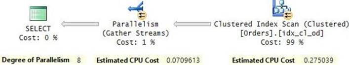
FIGURE 2-29 Parallel query plan with a scan.
With 272,000 rows, I still get a parallel plan. With 273,000 rows and beyond, I get a serial plan. For example, the following query got a serial plan on my system:
SELECT orderid, custid, empid, shipperid, orderdate, filler
FROM dbo.Orders
WHERE orderid <= 300000;
The execution plan I got for this query is shown in Figure 2-30.
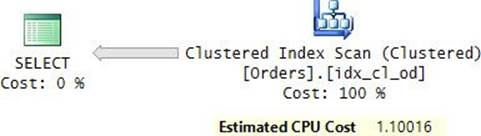
FIGURE 2-30 Serial query plan with a scan.
Because the costing formulas for parallel plans depend on the number of logical CPUs you have in the system, it can be tricky to troubleshoot a query on a test system that has a different number of CPUs than in the production system. There are a couple of tools you can use to make the optimizer assume a different number of CPUs than there really are, but unfortunately those tools are undocumented and unsupported, and their behavior should be considered unpredictable. So I use them strictly for experimentation and research purposes. I feel that experimenting with those tools helps me better understand how the SQL Server engine works, and I recommend that you refrain from using them in any capacity in production systems.
One tool is a DBCC command called OPTIMIZER_WHATIF. This tool makes the optimizer assume for the current session that the system has certain available resources just for costing purposes. To assume a certain number of CPUs, specify CPUs as the first parameter and the number as the second parameter. For example, to assume 16 CPUs, run the following code:
DBCC OPTIMIZER_WHATIF(CPUs, 16);
Examine the plan for the following query, which filters 300,000 rows:
SELECT orderid, custid, empid, shipperid, orderdate, filler
FROM dbo.Orders
WHERE orderid <= 300000
OPTION(RECOMPILE);
This time, I got a parallel plan. That’s because now CPUParallel is lower than before, allowing more rows to be filtered before reaching the tipping point between a parallel plan and a serial plan.
Note that this tool affects only the number of CPUs that will be considered for costing purposes; so the DOPForCosting measure will be computed as this number divided by 2, with integer division. The actual degree of parallelism for execution will still be based on the number of logical CPUs in the system. More precisely, it will be based on the number of schedulers that SQL Server creates; but normally, SQL Server creates one scheduler per logical CPU.
To revert back to the default number of CPUs in the system, specify 0 as the second parameter, like so:
DBCC OPTIMIZER_WHATIF(CPUs, 0);
The DBCC OPTIMIZER_WHATIF command has a local effect on the session. There’s a tool that has a more global impact on the entire system, but again, it’s undocumented and unsupported. As mentioned, normally SQL Server creates a scheduler for each logical CPU in the system, and the number of schedulers determines DOPForExecution. You can start the SQL Server service with startup parameter –Pn, where P has to be uppercase and n represents the number of schedulers you want SQL Server to use. You can query the sys.dm_os_schedulers view and filter only the rows with scheduler_id < 255 to see how many user schedulers SQL Server uses. Both the DOPForExecution measure and, consequently, the DOPForCosting measure will be determined by the number of schedulers, as if you have that many logical CPUs in the system. However, from a physical execution perspective, remember that you still have only as many CPUs as the number you actually have in the system.
Finally, a third undocumented and unsupported tool that affects parallelism treatment is query trace flag 8649. This trace flag causes SQL Server to use a parallel plan even if it has a higher cost than the alternative serial plan. Again, this is a tool I use for experimentation and research to see what the implications of using a parallel plan would be when SQL Server doesn’t choose one by itself. Here’s an example of using this trace flag in our query:
SELECT orderid, custid, empid, shipperid, orderdate, filler
FROM dbo.Orders
WHERE orderid <= 300000
OPTION(QUERYTRACEON 8649);
Remember that with 8 logical CPUs and the number of rows that this query filters, the optimizer would normally choose a serial plan. But with this trace flag, the optimizer chooses a parallel plan.
Unordered nonclustered index scan + lookups
The optimizer typically uses the unordered nonclustered index scan + lookups access method when the following conditions are in place:
![]() The query has a selective filter.
The query has a selective filter.
![]() There’s a nonclustered index that contains the filtered column (or columns), but the index isn’t a covering one.
There’s a nonclustered index that contains the filtered column (or columns), but the index isn’t a covering one.
![]() The filtered columns are not leading columns in the index key list.
The filtered columns are not leading columns in the index key list.
For example, the plan for the following query uses such an access method against the index idx_nc_sid_od_cid, created on the key columns (shipperid, orderdate, custid):
SELECT orderid, custid, empid, shipperid, orderdate, filler
FROM dbo.Orders
WHERE custid = 'C0000000001';
What’s important about this index is that the custid column appears in the index leaf rows but not as the first key column.
Figure 2-31 shows the query’s execution plan, and Figure 2-32 illustrates the way the storage engine processes the access method.
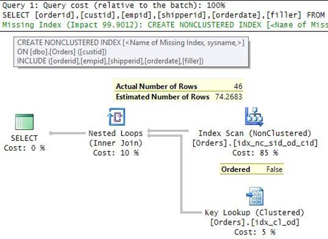
FIGURE 2-31 Unordered nonclustered index scan + lookups (execution plan).
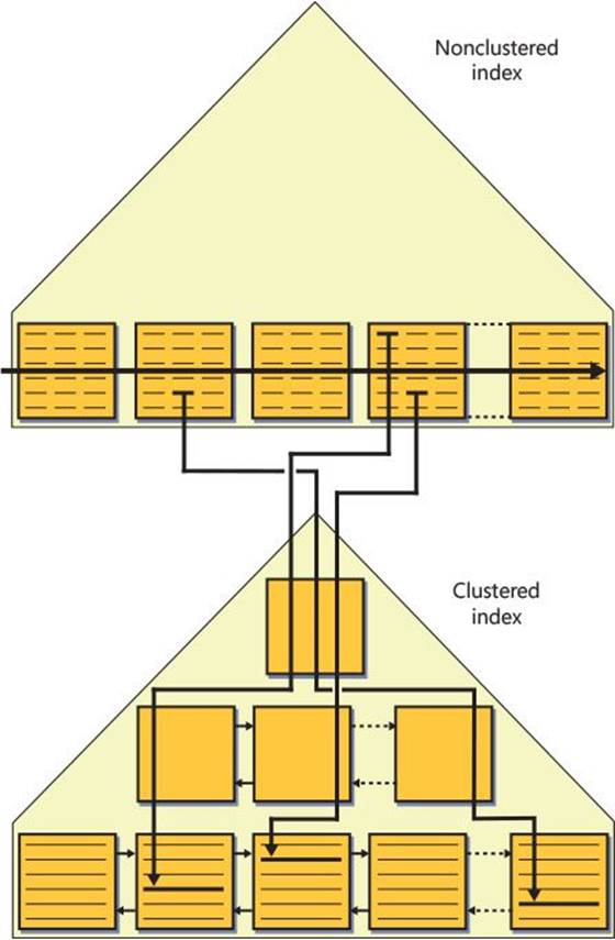
FIGURE 2-32 Unordered nonclustered index scan + lookups (storage engine).
SQL Server reported 4,006 logical reads for this query on my system.
Of course, you can get a much more efficient plan by creating a covering index with custid as the leading key column. Sure enough, the optimizer realizes this and reports such a missing index, as you can see in Figure 2-31. With such an index, you can get the desired result with probably three or four reads total. However, perhaps the query is so infrequent that you’d rather pay more when you do run it, but not incur the increase in the write costs resulting from the creation of another index. Also, perhaps you’re not allowed to create new indexes in the target system.
The unordered nonclustered index scan + lookups access method performs a full unordered scan of the leaf level of the index, followed by lookups for qualifying keys. As I mentioned, the query must be selective enough to justify this access method; otherwise, with too many lookups it will be more expensive than simply scanning the whole table. To figure out the cardinality of the filter, SQL Server needs a histogram on the filtered column. Normally, when you create an index, SQL Server creates statistics that include a histogram on the leading key column. But in our example, the optimizer needs a histogram on custid, which is not a leading key column in an index. If such statistics do not exist, SQL Server creates them, provided that the database property AUTO_CREATE_STATISTICS is turned on, which it is by default.
So when you ran this query for the first time, SQL Server looked for distribution statistics on the custid column and realized that none existed. SQL Server then checked the state of the AUTO_CREATE_STATISTICS database option and found that it was turned on. SQL Server then triggered an automatic creation of statistics based on the custid column after sampling a percentage of the values in the column. The optimizer then made a cardinality estimate for the filter based on the histogram, which as you can see in the query plan was 74.2683. That’s not very far from the actual number of matches, which is 46. Because of the selectivity of the filter, the optimizer estimated that using this access method is more efficient than using a full scan of the table. The scanning of the leaf level of the index cost 3,868 reads. The 46 key lookups cost 138 reads. That’s why in total the query performed 4,006 reads. Later in the chapter, I’ll elaborate on the cardinality estimation methods that the optimizer uses in the section “Cardinality estimates.”
Clustered index seek + range scan
As I explained when I described the access method nonclustered index seek + range scan + lookups, lookups are quite expensive. Therefore, when you have a nonclustered noncovering index, the optimizer typically uses it along with lookups only for a very small percentage of qualifying rows. I explained that there’s a tipping point beyond which the optimizer prefers a full scan of the table. If you have a query with a filter that tends to have a large number of matches and it’s important for you to get good performance, your focus should be on eliminating the need for the expensive lookups. This can be achieved by arranging a covering index—namely, an index that includes in the leaf row all columns that the query refers to. There are two main ways to get a covering index: one is with a clustered index, and another is with a nonclustered index with included columns. This section focuses on the former, and the next section focuses on the latter.
A clustered index is obviously a covering index because the leaf row is the complete data row. The optimizer typically uses the access method clustered index seek + range scan for range queries where you filter based on the first key column (or columns) of the clustered index. This access method performs a seek operation to the first qualifying row in the leaf level, and then it applies a range scan until the last qualifying row. Without the expensive lookups, this access method is always more efficient than an alternative full scan of the table. This makes a plan based on this method a trivial plan, meaning that there’s only one optimal plan for the query regardless of the number of matching rows.
The following query, which looks for all orders placed on a given orderdate (the clustered index key column), uses the access method, which is the focus of this discussion:
SELECT orderid, custid, empid, shipperid, orderdate
FROM dbo.Orders
WHERE orderdate = '20140212';
Figure 2-33 shows the query’s execution plan, and Figure 2-34 illustrates the way the storage engine processes the access method.
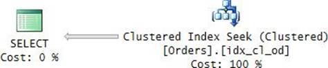
FIGURE 2-33 Clustered index seek + range scan (execution plan).
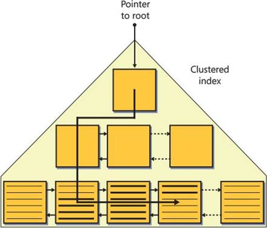
FIGURE 2-34 Clustered index seek + range scan (storage engine).
The filter uses an equality operator, but because the orderdate column isn’t unique, the filter might have multiple matching rows. In my case, I got 703 matching rows. SQL Server reported 22 logical reads for this query on my system. Naturally, you will get a similar access method if you use the operators >, >=, <, <=, and BETWEEN.
Covering nonclustered index seek + range scan
The access method covering nonclustered index seek + range scan is similar to the access method clustered index seek + range scan, only it uses a nonclustered covering index. The access method with the nonclustered index is more efficient because with fewer columns in the leaf row, you can fit more rows per leaf page. Take the query in the previous section as an example. The clustered index can fit about 40 rows per leaf page. This means that if the query has 10,000 matching rows, it needs to scan about 250 pages in the index leaf. To get an optimal covering nonclustered index, you create the index with orderdate as the key column, and specify all remaining columns from the query (orderid, custid, empid, and shipperid) in the index INCLUDE clause. The leaf row size in such an index is about 40 bytes, meaning that you can fit about 200 rows per leaf page; that’s compared to a leaf row size of about 200 bytes in the clustered index, with only 40 rows that fit in a leaf page. The row size ratio between the nonclustered index and the clustered index is one to five. This means that with the nonclustered index, the query can get the rows that it needs by scanning one-fifth of the pages compared to the clustered index. So, in the example with the 10,000 matching rows, the query would need to scan only about 50 pages in the nonclustered index leaf.
Besides coverage, there’s another critical thing you need to consider when optimizing queries with supporting indexes. When the query filter involves multiple predicates, you need to consider carefully the order of the key columns in the index key list. Take the following query as an example:
SELECT orderid, shipperid, orderdate, custid
FROM dbo.Orders
WHERE shipperid = 'C'
AND orderdate >= '20140101'
AND orderdate < '20150101';
The guidelines for the order of the key columns in the index key list depend on the operators you use in the predicates (equality or range) and, in some cases, the selectivity of the filter.
If you have multiple equality predicates, you have the most flexibility in creating an efficient index. You can define the key list in any order you like. That’s because with all key orders, the qualifying rows will appear in a consecutive range in the index leaf. For example, if the query filter was shipperid = <some_shipper_ID> AND orderdate = <some_date>, you can create the index with the key list (shipperid, orderdate) or (orderdate, shipperid).
You will hear some recommendations that claim you will get better cardinality estimates if you place the column from the more selective predicate first in the key list because the optimizer creates a histogram on the first key column. This is not really true, because as I explained earlier, if SQL Server needs a histogram on a column that is not a leading key in the index, it creates one on the fly. What could be a factor in determining key order when you use only equality predicates is if one column is always specified in the query filter and another only sometimes. You want to make sure that the column that is always specified appears first in the index key list because to get an index seek, the query filter has to refer to leading key columns.
If you have at most one range predicate and all remaining predicates are equality ones, you have less flexibility compared to having only equality predicates. However, you can still create an optimal index. The guideline in this case is to place the columns that appear in the equality predicates first in the key list (in any order that you like among them), and to place the column that appears in the range predicate last in the key list. Only this way will you get the qualifying rows in a consecutive range in the index leaf. Our sample query falls into this category because it has one equality predicate and one range predicate. As usual, if you want the index to be a covering one to avoid the need for lookups, place the remaining columns that appear in the query in the INCLUDE clause of the index. Following the indexing guidelines for this category, use the following code to create the optimal index:
CREATE INDEX idx_nc_sid_od_i_cid_orderid
ON dbo.Orders(shipperid, orderdate) INCLUDE(custid, orderid);
Figure 2-35 shows the execution plan for our sample query after creating this index, and Figure 2-36 illustrates the way the storage engine processes the access method.
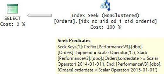
FIGURE 2-35 Covering nonclustered index seek + range scan (execution plan).
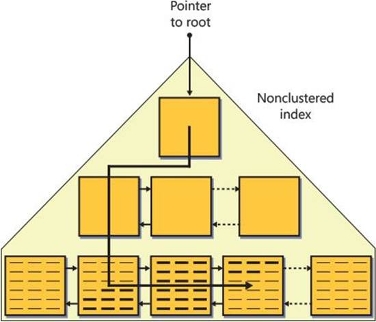
FIGURE 2-36 Covering nonclustered index seek + range scan (storage engine).
Observe the Seek Predicates property of the Index Seek operator in the plan: Prefix: shipperid = ‘C’, Start: orderdate >= ‘2014-01-01’, End: orderdate < ‘2015-01-01’. The seek operation finds the first row in the index leaf that satisfies the Prefix and Start predicates. The range scan continues until the last row that satisfies the Prefix and End predicates. When I ran this query on my system, I got 49,782 matching rows. SQL Server reported only 222 logical reads for the query. The range scan read only pages with qualifying rows. Had the index been created with the range column first in the key list and the equality column second, the situation would have been very different. SQL Server would have had to scan all rows that satisfy the range predicate (orderdate >= ‘20140101’ AND orderdate < ‘20150101’) as a seek predicate, and evaluate the equality predicate (shipperid = ‘C’) as a residual predicate.
If you have multiple range predicates, you’re not in luck. In such a case, it’s not possible to create an index that will arrange the qualifying rows in a consecutive range in the index leaf. Among the range predicates, only the one involving the leading key column among the ones that appear in the range predicates can be used as a seek predicate; all remaining range predicates will be used as residual predicates and will be applied to the scanned rows to determine whether to return them or not. For this reason, you want to make sure you place the column that is associated with the most selective range predicate right after the columns that are associated with equality predicates. Place all remaining columns from the range predicates last in the index key list.
For example, suppose that your filter has the predicates col1 > 5 AND col2 > 10. Suppose that the first predicate has 50 percent of matching rows and the second predicate has 2 percent. You want to make sure you define the index with the key list (col2, col1) and not the other way around. This way, SQL Server will need to scan only 2 percent of the pages in the index leaf instead of 50 percent. You will see a few examples in the book for performance problems that are associated with multiple range predicates and recommended ways to mitigate those problems. You will find such examples in Chapter 7, “Working with date and time,” in the discussion about intervals, and in Chapter 11, “Graphs and recursive queries,” in the discussion about the nested sets model.
To recap, when you have multiple equality predicates, place the columns from the predicates in any order that you like in the index key list. When you have at most one range predicate, place the columns from the equality predicates first in the key list and the column from the range predicate last. When you have multiple range predicates, place the column from the most selective range predicate before the columns from the remaining range predicates.
For more information about optimizing multiple predicates, see the series of articles “Optimization Tips for Multiple Range Predicates.” Part 1 can be found here: http://sqlmag.com/database-development/optimization-tips-multiple-range-predicates-part-1. Part 2 appears here:http://sqlmag.com/t-sql/optimization-tips-multiple-range-predicates-part-2. And Part 3 is here: http://sqlmag.com/t-sql/optimization-tips-multiple-range-predicates-part-3.
When you’re done, run the following code for cleanup:
DROP INDEX idx_nc_sid_od_i_cid_orderid ON dbo.Orders;
Cardinality estimates
The main component within the SQL Server relational engine (also known as the query processor) is the query optimizer. This component is responsible for generating physical execution plans for the queries you submit to SQL Server. During the optimization of a query, the optimizer explores alternative plans and chooses one that it considers to be the most efficient out of the ones that it explored. The optimizer needs to make decisions about which access methods to use to access objects, which join algorithms to use, which aggregate and distinct algorithms to use, how much memory to allocate for sort and hash activities, and so on. In many cases, the choices that the optimizer needs to make at different points in the plan depend on cardinality estimates—namely, on how many rows are returned from the previous operator. To make cardinality estimates, the optimizer employs a component called the cardinality estimator.
When you analyze a graphical query execution plan, you can see the cardinality estimates by placing your mouse pointer on the arrows coming out of the operators. If you examine an estimated query plan, you will see only estimates. If you examine an actual plan, you will see both the estimated numbers of rows and the actual numbers side by side. Often suboptimal choices that the optimizer makes are connected to inaccurate cardinality estimates, and the main way to detect those is by comparing the estimated and actual numbers. Note that the cost percentages associated with the different operators reflect the estimated costs that are connected to the estimated numbers of rows. Therefore, when the optimizer makes inaccurate estimates, those percentages can be misleading. Conversely, the thickness of the arrows in an actual plan reflects the actual number of rows flowing, so thicker arrows mean more rows flowing. Moreover, when you have a Nested Loops operator involved, be aware that the estimated number of rows reported for the inner part of the loop is for one execution, whereas the actual number of rows reported is the sum of all executions. So if you have a case where the estimated number of rows is 10, the estimated number of executions is 100, and the actual number of rows is 1,000, it’s actually an accurate estimate.
In the following sections, I go into the details of cardinality estimates. I cover major milestones in SQL Server regarding changes in the cardinality estimator, the implications of inaccurate estimates, statistics, multiple predicates, the ascending key problem, and the treatment of unknowns.
![]() Note
Note
As a reminder, I used randomization to create the sample data. Moreover, SQL Server samples only a percentage of the data using randomization when creating statistics for a column that is not a leading key in an index. So when you run the queries in my examples, you will most likely get slightly different results than mine.
Legacy estimator vs. 2014 cardinality estimator
The two major milestones for significant changes in the cardinality estimator were SQL Server 7.0 and SQL Server 2014. There’s a 16-year difference between the release dates of these versions. The new cardinality estimator is the result of lots of learning, taking into consideration the changes that took place over the years in database workloads. These days, the volume of data and the types of queries are different than they were two decades ago.
There are many changes in the new cardinality estimator compared to the legacy one. Microsoft’s goal was to improve the average case, with the understanding that there could be some cases with regression. SQL Server will use the new cardinality estimator by default when the database compatibility level is that of 2014 (120) or higher, and it will use the legacy estimator with lower compatibility levels. To make sure SQL Server uses the new cardinality estimator in our PerformanceV3 database, set the database compatibility level to 120 by running the following code:
USE PerformanceV3;
ALTER DATABASE PerformanceV3 SET COMPATIBILITY_LEVEL = 120;
If you identify certain queries that will benefit from the nondefault cardinality estimator, you can use a query trace flag to force a specific one. Use trace flag 9481 for the legacy cardinality estimator and trace flag 2312 for the new one. Because our database compatibility will cause SQL Server to use the new one by default, in my examples I will use query trace flag 9481 when I want to demonstrate using the old one. If you need your databases to use compatibility level 120 and up to enable new functionality but still use the old cardinality estimator by default, you can enable the trace flag at the server level with the startup parameter –T9481 or the command DBCC TRACEON(9481, –1).
I’m going to discuss a number of critical changes in cardinality estimation methods between the legacy estimator and the new cardinality estimator, but my coverage is not meant to be exhaustive. You can find more details in the following white paper: http://msdn.microsoft.com/en-us/library/dn673537.aspx.
Implications of underestimations and overestimations
Making accurate cardinality estimations is not a simple task you can do well without actually running the query and without a time machine. If you ever tried getting into the business of fortune telling, you know this. Even with the new cardinality estimator, you will still encounter cases where the estimations will be inaccurate. The implications of inaccurate estimations are generally that they might lead the optimizer to make suboptimal choices.
Underestimations and overestimations tend to have different implications. Underestimations will tend to result in the following (not an exhaustive list):
![]() For filters, preferring an index seek and lookups to a scan.
For filters, preferring an index seek and lookups to a scan.
![]() For aggregates, joins, and distinct, preferring order-based algorithms to hash-based ones.
For aggregates, joins, and distinct, preferring order-based algorithms to hash-based ones.
![]() For sort and hash operations, there might be spills to tempdb as a result of an insufficient memory grant.
For sort and hash operations, there might be spills to tempdb as a result of an insufficient memory grant.
![]() Preferring a serial plan over a parallel one.
Preferring a serial plan over a parallel one.
To demonstrate an underestimation, I’ll use a variable in the query and tell the optimizer to optimize the query for a specified value, like so:
DECLARE @i AS INT = 500000;
SELECT empid, COUNT(*) AS numorders
FROM dbo.Orders
WHERE orderid > @i
GROUP BY empid
OPTION(OPTIMIZE FOR (@i = 999900));
The execution plan for this query is shown in Figure 2-37.
FIGURE 2-37 Plan with underestimated cardinality.
As instructed, the optimizer optimized the query for the variable value 999900, regardless of the run-time value. The optimizer used the histogram on the orderid column to estimate the cardinality of the filter for this input, and it came up with an estimation of 100 rows. In practice, the filter has 500,000 matches. Consequently, you see all four aforementioned implications of an underestimation on the optimizer’s choices. It chose to use a seek in the index PK_Orders and lookups, even though a scan of the table would have been more efficient. It chose to sort the rows and use an order-based aggregate algorithm (Stream Aggregate) even though a hash aggregate would have been more efficient here. The memory grant for the sort operation was insufficient because it was based on the estimate of 100 rows, so the Sort operator ended up spilling to tempdb twice (spill level 2). It chose a serial plan even though a parallel plan would have been more efficient here.
Overestimations will tend to result in pretty much the inverse of underestimations (again, not an exhaustive list):
![]() For filters, preferring a scan to an index seek and lookups.
For filters, preferring a scan to an index seek and lookups.
![]() For aggregates, joins, and distinct, preferring hash-based algorithms to order-based ones.
For aggregates, joins, and distinct, preferring hash-based algorithms to order-based ones.
![]() For sort and hash operations, there won’t be spills, but very likely there will be a larger memory grant than needed, resulting in wasting memory.
For sort and hash operations, there won’t be spills, but very likely there will be a larger memory grant than needed, resulting in wasting memory.
![]() Preferring a parallel plan over a serial one.
Preferring a parallel plan over a serial one.
To demonstrate an overestimation, I’ll simply use a variable in the query and assign it a value that results in a selective filter, like so:
DECLARE @i AS INT = 999900;
SELECT empid, COUNT(*) AS numorders
FROM dbo.Orders
WHERE orderid > @i
GROUP BY empid;
Unlike parameter values, variable values normally cannot be sniffed. That’s because the initial optimization unit that the optimizer gets to work on is the entire batch. The optimizer is not supposed to execute the code preceding the query before optimizing it. In other words, it doesn’t perform the variable assignment before it optimizes the query. So it has to make a cardinality estimate for the predicate orderid > @i based on an unknown variable value. Later, in the section “Unknowns,” I provide a magic table of estimates for unknown inputs in Table 2-1. You will find that for the greater than (>) operator with an unknown input, the optimizer uses a hard-coded estimate of 30 percent matches. Apply 30 percent to the table’s cardinality of 1,000,000 rows, and you get 300,000 rows. That’s compared to an actual number of matches of 100. You can see these estimated and actual numbers in the execution plan for this query, which is shown in Figure 2-38.
FIGURE 2-38 Plan with overestimated cardinality.
You can see the aforementioned implications of an overestimation of cardinality on the optimizer’s choices. It chose to use a scan of some covering index instead of a seek in the index PK_Orders and lookups. It chose a local/global aggregate with a hash-based algorithm for the local aggregate instead of using an order-based aggregate. The memory grant for the hash and sort operations is exaggerated. It chose a parallel plan instead of a serial one.
Of course, it is best if the cardinality estimate is accurate, but between an underestimation and an overestimation, I generally prefer the latter. That’s because I find that the impact of an overestimation on the performance of the query tends to be less severe.
Statistics
SQL Server relies on statistics about the data in its cardinality estimates. Whenever you create an index, SQL Server creates statistics using a full scan of the data. When additional statistics are needed, SQL Server might create them automatically using a sampled percentage of the data. SQL Server creates three main types of statistics: header, density vectors, and a histogram. To demonstrate those, run the following code, which creates an index with the key columns (custid, empid):
CREATE INDEX idx_nc_cid_eid ON dbo.Orders(custid, empid);
SQL Server created the three aforementioned types of statistics to support the index. You can see those by running the DBCC SHOW_STATISTICS command, like so:
DBCC SHOW_STATISTICS(N'dbo.Orders', N'idx_nc_cid_eid');
I got the following output from this command (with the text for the header wrapped to fit in print):
Name Updated Rows Rows Sampled Steps Density Average key length
--------------- -------------------- -------- ------------- ------ ----------- ------------------
idx_nc_cid_eid Oct 21 2014 7:17PM 1000000 1000000 187 0.02002646 18
String Index Filter Expression Unfiltered Rows
------------- ------------------ ----------------
YES NULL 1000000
All density Average Length Columns
------------- -------------- -------------------------
5E-05 11 custid
1.050216E-06 15 custid, empid
1.000042E-06 18 custid, empid, orderdate
RANGE_HI_KEY RANGE_ROWS EQ_ROWS DISTINCT_RANGE_ROWS AVG_RANGE_ROWS
------------ ------------- ------------- -------------------- --------------
C0000000001 0 46 0 1
C0000000130 6437 37 128 50.28906
C0000000252 6089 37 121 50.32232
C0000000310 2918 67 57 51.19298
C0000000539 11538 62 228 50.60526
...
C0000019486 6307 66 126 50.05556
C0000019704 10934 30 217 50.3871
C0000019783 4045 66 78 51.85897
C0000019904 5906 68 120 49.21667
C0000020000 4733 46 95 49.82105
The first part in the statistics is the header. It contains general information about the data, such as the cardinality of the table (1,000,000 rows in our example).
The second part in the statistics is the density vectors. This part records density information for all leading vectors of key columns. You created the index on custid and empid, but internally SQL Server added orderdate as the last key column; that’s because the orderdate column is the clustered index key column and therefore nonclustered indexes use it as the row locator. So, with three key columns, you have three vectors of leading columns. The density of the column represents the average percentage of occurrences per distinct combination of values. For example, there are 20,000 distinct customer IDs in the table, so the average percentage per distinct value is 1 / 20,000 = 0.00005, or 5E-05 as it appears in the statistics. As you add more columns, the density reduces until you get uniqueness. So, for the vector (custid, empid), the density is 0.000001050216, or 1.050216E-06. SQL Server uses the density information when it needs to make cardinality estimates for unknown inputs, or when it considers that the average case is likely to be more accurate.
The third part of the statistics is the histogram. When you create an index, SQL Server creates a histogram on the leading key based on a full scan of the data. In addition, when SQL Server optimizes a query and needs a histogram on a column that is not a leading index key, it can create one on the fly as long as the database option AUTO_CREATE_STATISTICS is enabled. It samples a percentage of the rows for this purpose.
SQL Server supports only single-column histograms with up to 200 steps. Each step represents the range of keys that are greater than the previous step’s RANGE_HI_KEY value and less than or equal to the current RANGE_HI_KEY value. For example, the second step in our histogram represents the range of customer IDs that are greater than C0000000001 and less than or equal to C0000000130. The RANGE_ROWS value indicates the number of rows represented by the step, excluding the ones with the RANGE_HI_KEY value. The EQ_ROWS value represents the number of rows with the RANGE_HI_KEY value. The sum of RANGE_ROWS and EQ_ROWS is the total number of rows that the step represents. The DISTINCT_RANGE_ROWS value represents the distinct count of the key values in the step, excluding the upper bound. The AVG_RANGE_ROWSvalue represents the average number of rows in the step per distinct key value, again, excluding the upper bound.
SQL Server uses the histogram to make cardinality estimates for known inputs. As an example, consider the following query:
SELECT orderid, custid, empid, shipperid, orderdate, filler
FROM dbo.Orders
WHERE custid = 'C0000000001';
The execution plan for this query is shown in Figure 2-39.
FIGURE 2-39 Plan that shows the use of a histogram on a single column based on RANGE_HI_KEY.
SQL Server looked for the step responsible for the input value C0000000001 and found that it belongs to step 1. It so happens that this input value is equal to the RANGE_HI_KEY value in the step, so the cardinality estimate for it is simply the EQ_ROWS value, which is 46. You can see in the query plan that 46 is the estimated number of rows after filtering.
As another example, consider the following query:
SELECT orderid, custid, empid, shipperid, orderdate, filler
FROM dbo.Orders
WHERE custid = 'C0000000002';
Observe the first two steps in the histogram:
RANGE_HI_KEY RANGE_ROWS EQ_ROWS DISTINCT_RANGE_ROWS AVG_RANGE_ROWS
------------ ------------- ------------- -------------------- --------------
C0000000001 0 46 0 1
C0000000130 6437 37 128 50.28906
The input value belongs to step 2. However, it is less than the RANGE_HI_KEY value of the step, so SQL Server uses the AVG_RANGE_ROWS value of 50.2891 as the cardinality estimate. The query plan I got for this query on my system showed an estimated number of rows of 50.2891 and an actual number of 57.
As you can see, with an equality predicate for a known input the cardinality estimate is pretty straightforward. If you have a range predicate, the estimate will be interpolated from the information in the histogram steps. If only one step is involved, the estimate will be interpolated from only that step’s information. If multiple steps are involved, SQL Server will split the filter’s range into the subintervals that intersect with the different steps, interpolate the estimate for each subinterval, and aggregate the estimates.
The next example demonstrates a case where the optimizer uses density vectors. Remember that unlike parameter values, variable values aren’t sniffable. That’s because the initial optimization unit is the batch and the optimizer isn’t supposed to execute the assignments before it optimizes the query. Consider the following code:
DECLARE @cid AS VARCHAR(11) = 'C0000000001';
SELECT orderid, custid, empid, shipperid, orderdate, filler
FROM dbo.Orders
WHERE custid = @cid;
The optimizer cannot sniff the variable value here. Because density information is available for the custid column, the optimizer uses it. Remember that the density for this column is 0.00005. Multiply this value by the table’s cardinality of 1,000,000 rows, and you get 50. The execution plan I got for this query showed an estimated number of rows of 50 and an actual number of 46.
Estimates for multiple predicates
As mentioned, SQL Server supports only single-column histograms. When the query filter involves more than one predicate, SQL Server can make an estimate for each of the predicates based on the respective histogram, but it will need to somehow combine the estimates into a single one. The legacy estimator and new cardinality estimator handle this differently.
I’ll explain the estimation methods with both a conjunction of predicates (predicates separated by AND operators) and a disjunction of predicates (predicates separated by OR operators).
Before I describe estimation methods for multiple predicates, I’ll make a note of the selectivity (percentage of matches) of two specific predicates so that I can use those in my examples. The following query has a filter with a predicate based on the custid column:
SELECT orderid, custid, empid, shipperid, orderdate, filler
FROM dbo.Orders
WHERE custid <= 'C0000001000';
On my system, the query plan shows an estimated number of rows of 52,800. This number translates to a selectivity of 5.28%.
The following query has a filter with a predicate based on the empid column:
SELECT orderid, custid, empid, shipperid, orderdate, filler
FROM dbo.Orders
WHERE empid <= 100;
If there are no statistics on the empid column before you run this query, the execution of this query triggers the creation of such statistics. On my system, the query plan showed an estimated number of rows of 19,800, translating to a selectivity of 19.8%.
The legacy cardinality estimator assumes that when your query has multiple predicates, they are independent of each other. Based on this assumption, for a conjunction of predicates it computes the result selectivity as the product of the individual ones. Consider the following query as an example (notice the trace flag forces the use of the legacy cardinality estimator):
SELECT orderid, custid, empid, shipperid, orderdate, filler
FROM dbo.Orders
WHERE custid <= 'C0000001000'
AND empid <= 100
OPTION(QUERYTRACEON 9481);
On my system, I got the query plan shown in Figure 2-40.
FIGURE 2-40 Estimate for the conjunction with the legacy cardinality estimator.
Remember that the individual estimates on my system were 5.28% and 19.8%, so the product is 5.28% * 19.8% = 10.4%. Indeed, the cardinality estimate in the plan reflects this.
After many years of experience with SQL Server, Microsoft learned that, in reality, there’s usually some level of dependency between predicates. In the average case, predicates are neither completely independent nor completely dependent—rather, they are somewhere in between. Even though my sample data doesn’t reflect this because I used simple randomization to create it, if you think about it, there will typically be some dependency between the customer who places an order and the employee who handles it. With complete independence, statistically a product of the individual estimates should be used. Under complete dependence, the most selective estimate should be used. But because the average case in reality is somewhere in between, Microsoft chose a method called exponential backoff, which is suitable in such a case. This method takes into consideration the most selective estimate as is, and then gradually reduces the effect of the less selective estimates by raising each to the power of a smaller fraction. Assuming S1 is the most selective estimate (expressed as a percentage), S2 is the next most selective, and so on, the exponential backoff formula is the following:
S1 * S21/2 * S31/4 * S41/8 * ...
Of course, the cardinality estimator will multiply the final percentage by the input’s cardinality (1,000,000 in our case) to produce an estimate in terms of a number of rows. In our example, when you apply this method to our two predicates, you get 5.28% * SQRT(19.8%) = 23.5%, which translates to 23,500 rows.
Here’s our query without the trace flag, meaning that the new cardinality estimator will be used:
SELECT orderid, custid, empid, shipperid, orderdate, filler
FROM dbo.Orders
WHERE custid <= 'C0000001000'
AND empid <= 100;
I got the plan shown in Figure 2-41.
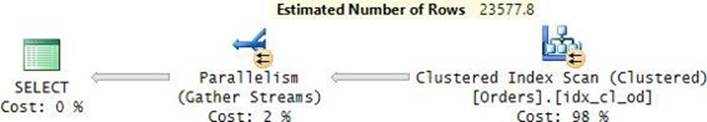
FIGURE 2-41 Estimate for the conjunction with the new cardinality estimator.
As you can see, the cardinality estimate here was based on the exponential backoff method, and as a result, you get a higher estimate compared to the legacy method, which is based on a simple product. If you have cases where predicates are truly independent of each other, you can always add trace flag 9481 to the query to force the legacy cardinality estimation method.
For a disjunction of predicates, the legacy cardinality estimator computes the sum of the individual estimates minus their product. Consider the following query as an example:
SELECT orderid, custid, empid, shipperid, orderdate, filler
FROM dbo.Orders
WHERE custid <= 'C0000001000'
OR empid <= 100
OPTION(QUERYTRACEON 9481);
The estimate in this example is computed as 5.28% + 19.8% – (5.28% * 19.8%) = 24%.
The new cardinality estimator uses a method that is more aligned with the method for a conjunction of predicates. It negates (100% minus) the result of an exponential backoff formula that is based on the negation of the individual estimates. In our example, this translates to 100% – (100% – 19.8%) * SQRT(100% – 5.28%) = 21.9%. That’s the estimate I got on my system for our sample query (about 21,900 rows):
SELECT orderid, custid, empid, shipperid, orderdate, filler
FROM dbo.Orders
WHERE custid <= 'C0000001000'
OR empid <= 100;
If you have multiple predicates and you often get inaccurate estimates there are a couple of ways to get better estimates. That’s assuming that all predicates are equality ones or that you have at most one range predicate but all the rest are equality ones. For example, suppose that users often filter the data by customer ID and employee ID, both with equality predicates. So the query filter might look like this: WHERE custid = ‘C0000000003’ AND empid = 5. You create a computed column (call it custid_empid) that concatenates the customer ID and employee ID values. Just the fact that a computed column exists allows SQL Server to create statistics on the column, regardless of whether you index it or not. Your query will need to filter the concatenated value to benefit from such statistics. You can filter by the computed column name or directly by the concatenated expression. In both cases, SQL Server can rely on the histogram on the computed column and on an index if you created one. So the query filter might look like this: WHERE custid_empid = ‘C0000000003_5’.
Another method to use to get better estimates is working with filtered indexes. As long as you have a small number of distinct values in one of the columns, a solution that creates a filtered index per distinct value is maintainable. For example, suppose that in your organization only 10 distinct employees handle orders; in such a case, it’s reasonable to create 10 filtered indexes, one per distinct employee ID. For example, the index for employee ID 5 will have the filter WHERE empid = 5. The index key will be based on the custid column. SQL Server will create a histogram based on the custid column for each filtered index. When the optimizer will need to make a cardinality estimate for a filter such as WHERE custid = ‘C0000000003’ AND empid = 5, it will use the histogram on the custid column in the filtered index for that employee ID (in this example, 5). Effectively, the quality of the estimates will be the same as if you had a multicolumn histogram. You can find more information on filtered indexes later in the chapter, in the section “Indexing features.”
When you’re done, run the following code for cleanup:
DROP INDEX idx_nc_cid_eid ON dbo.Orders;
Ascending key problem
SQL Server normally refreshes statistics once every 500 plus 20 percent of changes in the column in question. Any data added after the statistics were last refreshed is not modeled by the statistics. As an example, the following code creates a table called Orders2 with 900,000 rows and a nonclustered index through a primary key constraint called PK_Orders2:
IF OBJECT_ID(N'dbo.Orders2', N'U') IS NOT NULL DROP TABLE dbo.Orders2;
SELECT * INTO dbo.Orders2 FROM dbo.Orders WHERE orderid <= 900000;
ALTER TABLE dbo.Orders2 ADD CONSTRAINT PK_Orders2 PRIMARY KEY NONCLUSTERED(orderid);
SQL Server creates statistics for the index as part of the index creation; therefore, the histogram on the orderid column models all 900,000 rows from the table. Run the following code to show the statistics for the index:
DBCC SHOW_STATISTICS('dbo.Orders2', 'PK_Orders2');
I got the following output on my system:
Name Updated Rows Rows Sampled Steps Density Average key length
----------- -------------------- ------- ------------- ------ -------- ------------------
PK_Orders2 Oct 21 2014 9:29PM 900000 900000 2 1 4
String Index Filter Expression Unfiltered Rows
------------ ------------------ ----------------
NO NULL 900000
All density Average Length Columns
------------- -------------- --------
1.111111E-06 4 orderid
RANGE_HI_KEY RANGE_ROWS EQ_ROWS DISTINCT_RANGE_ROWS AVG_RANGE_ROWS
------------ ------------- ------------- -------------------- --------------
1 0 1 0 1
900000 899998 1 899998 1
The last part of the output is the histogram on the orderid column. Observe that the maximum order ID value recorded is 900,000, which is indeed currently the maximum value in the table. Next, run the following code to add 100,000 rows:
INSERT INTO dbo.Orders2
SELECT *
FROM dbo.Orders
WHERE orderid > 900000 AND orderid <= 1000000;
Now query the table and filter the rows with an order ID that is greater than 900,000, like so (the trace flag ensures the legacy cardinality estimator is used):
SELECT orderid, custid, empid, shipperid, orderdate, filler
FROM dbo.Orders2
WHERE orderid > 900000
ORDER BY orderdate
OPTION(QUERYTRACEON 9481);
Because the extra 100,000 rows are less than the threshold for refreshing the statistics, the new rows are not modeled by the histogram. You can see this by running DBCC SHOW_STATISTICS again. You will see that the maximum value is still 900,000. The legacy cardinality estimator examines the histogram and sees that the filter’s range is after the maximum value in the histogram. Based on just this information, the estimate should be zero matching rows, but the minimum allowed estimation is 1. Examine the execution plan for the query in Figure 2-42.
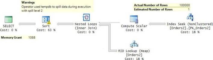
FIGURE 2-42 Plan showing the ascending key problem with the legacy cardinality estimator.
Observe that the estimated cardinality of the filter is 1 row, whereas the actual is 100,000. You can see a number of suboptimal choices that the optimizer made based on the inaccurate estimate. This problem typically happens when the column is an ascending key column and you filter recent data. Often the recent data isn’t modeled by the histogram.
The new cardinality estimator handles the estimate differently. If it identifies that the filter’s interval exceeds the recorded maximum, it interpolates the estimate by taking into consideration the count of modifications since the last statistics refresh. Run the sample query again, but this time allow SQL Server to use the new cardinality estimator:
SELECT orderid, custid, empid, shipperid, orderdate, filler
FROM dbo.Orders2
WHERE orderid > 900000
ORDER BY orderdate;
I got the execution plan shown in Figure 2-43.
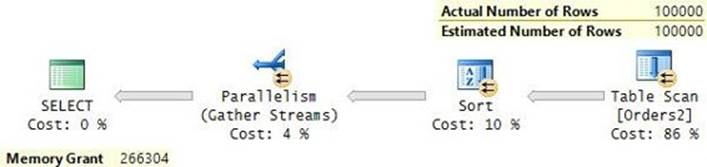
FIGURE 2-43 Plan showing the ascending key problem solved with the new cardinality estimator.
This time, as you can see, the estimate is accurate. As a result, the choices that the optimizer made are much more optimal.
Another tool you can use to deal with the ascending key problem is trace flag 2389. Unlike the new cardinality estimator, this trace flag is available prior to SQL Server 2014. If you enable this trace flag, when SQL Server refreshes statistics it checks if the values in the source column keep increasing. If they keep increasing in three consecutive refreshes, SQL Server brands the source column as ascending. Then, at query compile time, SQL Server adds a ministep to the histogram to model the data that was added since the last refresh. You can find information about this trace flag here: http://blogs.msdn.com/b/ianjo/archive/2006/04/24/582227.aspx.
With very large tables, the default threshold for an automatic statistics update of every 500 plus 20 percent of changes could be insufficient. Think about it: for a table with 100,000,000 rows, the threshold is 20,000,500 changes. If you enable trace flag 2371, SQL Server will gradually reduce the percentage as the table grows. You can find details about this trace flag, including a graph showing the gradual change, here: http://blogs.msdn.com/b/saponsqlserver/archive/2011/09/07/changes-to-automatic-update-statistics-in-sql-server-traceflag-2371.aspx.
Unknowns
I described some cardinality estimation methods SQL Server uses when statistics are available and the input values are known (for example, when you use constants or parameters). In some cases, SQL Server uses cardinality estimation methods based on unknown inputs. Following are those cases:
![]() No statistics are available.
No statistics are available.
![]() You use variables (as opposed to parameters). As mentioned earlier, variable values aren’t sniffable because the initial optimization unit is the entire batch.
You use variables (as opposed to parameters). As mentioned earlier, variable values aren’t sniffable because the initial optimization unit is the entire batch.
![]() You use parameters with sniffing disabled (for example, when you specify the OPTIMIZE FOR UNKNOWN hint).
You use parameters with sniffing disabled (for example, when you specify the OPTIMIZE FOR UNKNOWN hint).
Table 2-1 shows the rules that SQL Server uses to make a cardinality estimate for unknown inputs based on the operator you use.
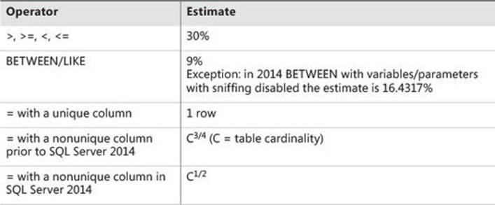
TABLE 2-1 Magic table of estimates for unknown inputs
I should mention that there are a couple of exceptional cases in which SQL Server won’t use this table. One exception is with variables. I mentioned that normally variable values aren’t sniffable. However, if you force a statement-level recompile with a RECOMPILE query option or an automatic statement-level recompile happens, the query gets optimized after the variable values are assigned. Therefore, the variable values become sniffable to the optimizer, and then SQL Server can use its normal cardinality estimation methods based on statistics.
The other exception is when using variables or parameters with sniffing disabled, and the operator is an equality operator, and a density vector is available for the filtered columns. In such a case, the estimate will be based on the density vector.
Next, I’ll demonstrate examples for estimates that are based on the rules in Table 2-1. Run the following code to check which indexes you currently have on the Orders table:
EXEC sp_helpindex N'dbo.Orders';
The output should show only the following indexes:
idx_cl_od
idx_nc_sid_od_cid
idx_unc_od_oid_i_cid_eid
PK_Orders
If you get any other indexes, drop them.
Run the following code to turn off the auto collection of statistics in the database:
ALTER DATABASE PerformanceV3 SET AUTO_CREATE_STATISTICS OFF;
Run the following query to identify statistics that were created automatically on the Orders table:
SELECT S.name AS stats_name,
QUOTENAME(OBJECT_SCHEMA_NAME(S.object_id)) + N'.' + QUOTENAME(OBJECT_NAME(S.object_id)) AS
object,
C.name AS column_name
FROM sys.stats AS S
INNER JOIN sys.stats_columns AS SC
ON S.object_id = SC.object_id
AND S.stats_id = SC.stats_id
INNER JOIN sys.columns AS C
ON SC.object_id = C.object_id
AND SC.column_id = C.column_id
WHERE S.object_id = OBJECT_ID(N'dbo.Orders')
AND auto_created = 1;
Drop all statistics that this query reports. In my case, I used the following code based on the output of the query; of course, you should drop the statistics that the query reports for you:
DROP STATISTICS dbo.Orders._WA_Sys_00000002_38EE7070;
DROP STATISTICS dbo.Orders._WA_Sys_00000003_38EE7070;
Observe in Table 2-1 that the estimate for unknown with any of the operators >, >=, <, <= is 30%. The following queries demonstrate this estimation method:
-- Query 1
DECLARE @i AS INT = 999900;
SELECT orderid, custid, empid, shipperid, orderdate, filler
FROM dbo.Orders
WHERE orderid > @i;
-- Query 2
SELECT orderid, custid, empid, shipperid, orderdate, filler
FROM dbo.Orders
WHERE custid <= 'C0000000010';
Figure 2-44 shows the plans for these queries.
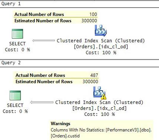
FIGURE 2-44 Plans showing an estimate of 30 percent.
The first query uses a variable whose value cannot be sniffed. The second uses a constant, but statistics are not available, and you disabled the option to create new ones.
For the BETWEEN and LIKE predicates, Table 2-1 shows an estimate of 9%. An exception to this rule is that in SQL Server 2014 when you use BETWEEN with variables, or parameters with sniffing disabled, the estimate is 16.4317%. The following queries demonstrate these rules:
-- Query 1
DECLARE @i AS INT = 999901, @j AS INT = 1000000;
SELECT orderid, custid, empid, shipperid, orderdate, filler
FROM dbo.Orders
WHERE orderid BETWEEN @i AND @j;
-- Query 2
SELECT orderid, custid, empid, shipperid, orderdate, filler
FROM dbo.Orders
WHERE orderid BETWEEN @i AND @j
OPTION(QUERYTRACEON 9481);
-- Query 3
SELECT orderid, custid, empid, shipperid, orderdate, filler
FROM dbo.Orders
WHERE custid BETWEEN 'C0000000001' AND 'C0000000010';
-- Query 4
SELECT orderid, custid, empid, shipperid, orderdate, filler
FROM dbo.Orders
WHERE custid LIKE '%9999';
The execution plans for these queries are shown in Figure 2-45.
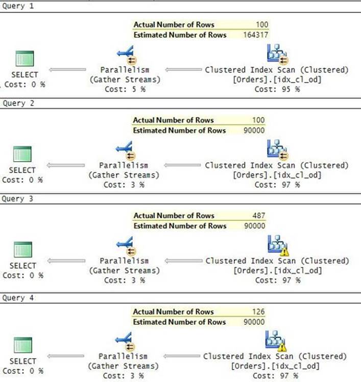
FIGURE 2-45 Plans showing estimates for BETWEEN and LIKE.
The first query falls into the exception that I just described, so it gets an estimate of 16.4317%. The second query is the same as the first, but because you force using the legacy cardinality estimator, you get an estimate of 9%. The third and fourth queries use constants, but there are no statistics available. As an aside, query 4 normally causes string statistics, which contain information about occurrences of substrings, to be created. However, because you disabled automatic creation of statistics in the database, SQL Server did not create those statistics, and it used the estimation method based on unknown inputs instead.
With the equality operator, the estimation method for an unknown input depends on the uniqueness of the column and the version of SQL Server. When the column is unique, the estimate is 1 row. When it’s not unique, in SQL Server 2014 the estimate is C1/2, where C is the input’s cardinality, and prior to SQL Server 2014 it’s C3/4.
The following queries demonstrate all three methods:
-- Query 1
DECLARE @i AS INT = 1000000;
SELECT orderid, custid, empid, shipperid, orderdate, filler
FROM dbo.Orders
WHERE orderid = @i;
-- Query 2
SELECT orderid, custid, empid, shipperid, orderdate, filler
FROM dbo.Orders
WHERE custid = 'C0000000001';
-- Query 3
SELECT orderid, custid, empid, shipperid, orderdate, filler
FROM dbo.Orders
WHERE custid = 'C0000000001'
OPTION(QUERYTRACEON 9481);
The execution plans with the estimates for these queries are shown in Figure 2-46.
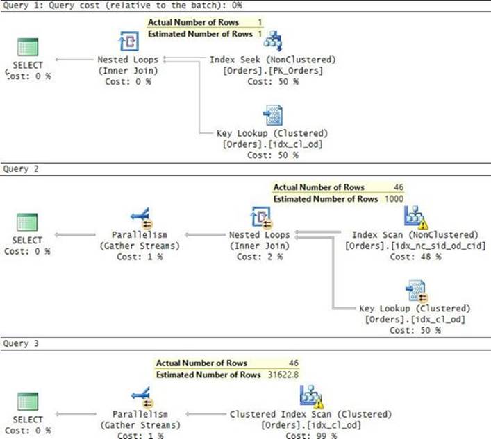
FIGURE 2-46 Plans showing estimates for equality.
When you’re done experimenting, run the following code to turn the automatic creation of statistics back on:
ALTER DATABASE PerformanceV3 SET AUTO_CREATE_STATISTICS ON;
Feel free to rerun the queries to see how the estimations change when SQL Server automatically creates statistics when it needs those. For example, rerun the query with the LIKE predicate:
SELECT orderid, custid, empid, shipperid, orderdate, filler
FROM dbo.Orders
WHERE custid LIKE '%9999';
I got the query plan shown in Figure 2-47.
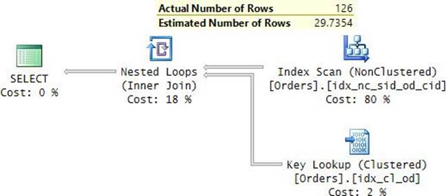
FIGURE 2-47 Plan for a query using LIKE with string statistics available.
SQL Server first created string statistics on the custid column and then performed the estimate based on those statistics. Compared to the previous estimate you got for this query in Figure 2-45 (it was Query 4 in that figure), this time the estimate is much more accurate.
Another curious difference between the legacy and new cardinality estimators is in how they handle a filter with an expression that manipulates a column. Take the expression orderid % 2 = 0 as an example. The legacy cardinality estimator simply treats the case as an unknown input. As such, the estimate for an equality operator is C3/4. With our Orders table, this translates to 1,000,0003/4 = 31,622. That’s likely to be a significant underestimation. The new cardinality estimator is more sophisticated. Here, it actually realizes that the expression uses the modulo (%) operator. Statistically, with % 2 = 0, you’re going to get 50% matches. Accordingly, the estimation for this case is 500,000 rows. This will likely be much closer to the actual number than the estimation made by the legacy cardinality estimator.
Indexing features
This section covers various indexing features. It includes information about descending indexes, included non-key columns, filtered indexes and statistics, columnstore indexes, and inline index definition. The features are covered in the order in which they were added to SQL Server.
Descending indexes
With SQL Server, you can indicate the direction of key columns in an index definition. By default, the direction is ascending, but using the DESC keyword you can request descending order, as in (col1, col2 DESC).
Indexes on disk-based tables have a doubly linked list in their leaf level. So SQL Server can scan the rows in the leaf in forward and backward order. As an aside, as you will learn in Chapter 10, BW-Tree indexes on memory-optimized tables are unidirectional. But back to B-tree-based indexes on disk-based tables, at the beginning it might seem like there’s no need for descending indexes, but there are a few use cases.
As it turns out, the storage engine is currently able to process only forward scans with parallelism. Whenever you have a backward scan, it is processed serially. Take the following queries as an example:
-- Query 1, parallel
SELECT orderid, custid, empid, shipperid, orderdate, filler
FROM dbo.Orders
WHERE orderid <= 100000
ORDER BY orderdate;
-- Query 2, serial
SELECT orderid, custid, empid, shipperid, orderdate, filler
FROM dbo.Orders
WHERE orderid <= 100000
ORDER BY orderdate DESC;
Figure 2-48 shows the execution plans for these queries.
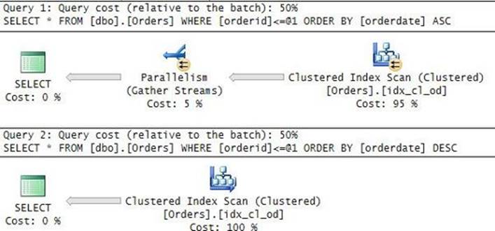
FIGURE 2-48 Plans showing that there’s no parallel backward scan.
I have 8 logical CPUs on my machine. According to SQL Server’s costing formulas, with that many CPUs, a query against a table with 1,000,000 rows that filters 100,000 rows should get a parallel plan. That’s why the plan for the first query uses a parallel scan. However, because a backward scan cannot be processed with parallelism, the plan for the second query uses a serial one.
It’s interesting to see what the optimizer does when you try to force parallelism with the second query using query trace flag 8649, like so:
SELECT orderid, custid, empid, shipperid, orderdate, filler
FROM dbo.Orders
WHERE orderid <= 100000
ORDER BY orderdate DESC
OPTION(QUERYTRACEON 8649);
The plan for this query is shown in Figure 2-49.
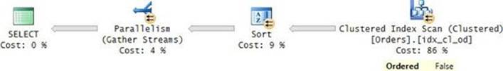
FIGURE 2-49 Plan with forced parallelism.
Not being able to use a parallel backward-order scan, the optimizer chose a plan that uses a parallel unordered scan, and then an explicit sort operation. Clearly, it’s a very inefficient plan. If you find that parallelism is a critical factor in the performance of the query, you can arrange a descending index. Of course, if at some point Microsoft introduces support for parallel backward scans, you won’t need descending indexes for this purpose anymore.
Another curious case where descending indexes are useful is with window functions that have both a window partition clause and a window order clause. Consider the following queries:
-- Query 1
SELECT shipperid, orderdate, custid,
ROW_NUMBER() OVER(PARTITION BY shipperid ORDER BY orderdate) AS rownum
FROM dbo.Orders;
-- Query 2
SELECT shipperid, orderdate, custid,
ROW_NUMBER() OVER(PARTITION BY shipperid ORDER BY orderdate DESC) AS rownum
FROM dbo.Orders;
-- Query 3
SELECT shipperid, orderdate, custid,
ROW_NUMBER() OVER(PARTITION BY shipperid ORDER BY orderdate DESC) AS rownum
FROM dbo.Orders
ORDER BY shipperid DESC;
Currently, there is a covering index called idx_nc_sid_od_cid on the table, defined with the key list (shipperid, orderdate, custid). Examine the execution plans for these queries as shown in Figure 2-50.
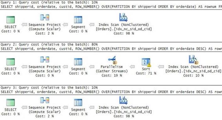
FIGURE 2-50 Plans for queries with a window function.
The plan for query 1 shows that as long as there’s a covering index with a key list that starts with the partition columns in ascending order, and continues with the order columns in the order specified in the window function, the optimizer chooses an ordered scan of the index and avoids an explicit sort operation.
In query 2, the window function’s specification is similar to the one in query 1, but with descending order for the window order column orderdate. Theoretically, the optimizer could have chosen a plan that scans our covering index in descending order. After all, absent a presentation ORDER BY clause, SQL Server might return the rows in any order in the output. But it seems like SQL Server somehow wants to process the rows in ascending order of the window partition elements, so it adds an explicit sort operation.
Oddly, as you can see in the plan for query 3, if you do add a presentation ORDER BY clause with the shipperid column in descending order, suddenly the optimizer figures that it can use a backward scan both to compute the window function and to support the desired presentation order. I learned this last bit from Brad Shultz, mind you, while presenting a session in front of hundreds of people.
Another use case for descending indexes is when SQL Server needs to process rows based on multiple columns with opposite directions. For example, if your query has an ORDER BY clause with col1, col2 DESC, it can benefit from an index with the key list col1, col2 DESC or col1 DESC, col2. An index with both columns in ascending order isn’t optimal; SQL Server would still need to explicitly sort the rows.
As an anecdote, almost two decades ago, shortly after SQL Server 2000 was released, my friend Wayne Snyder discovered one of the most amazing bugs I’ve seen in SQL Server. If you created a clustered index with col1 DESC as the key, and issued a DELETE statement with the filtercol1 > @n, SQL Server deleted all rows where col1 < @n. This bug existed in SQL Server 2000 RTM and, of course, was fixed in Service Pack 1.
Included non-key columns
When you define a nonclustered index, you specify a vector of columns as the key list to determine the order of the rows in the index. SQL Server can perform ordered scans and range scans based on this key list to support operations such as ordering, filtering, grouping, joining, and others. However, if you need to add columns to the index for coverage purposes (to avoid lookups) and those columns don’t serve any ordering-related purpose, you add those columns in a designated INCLUDE clause.
Unlike key columns, included columns appear only in the index leaf rows. Also, SQL Server imposes fewer restrictions on those. For example, the key list cannot have more than 16 columns, whereas included columns can. The key list cannot have more than 900 bytes, whereas included columns can. The key list cannot have special types like XML and other large object types, whereas the include list can. Moreover, when you update a row in the table, naturally SQL Server needs to update all respective index rows that contain the updated columns. If an index key column value changes, the sort position of the row might change, in which case SQL Server will need to relocate the row. If an included column value changes, the sort position remains the same, and the update can happen in place (assuming the row doesn’t expand).
As an example for a use case for the INCLUDE clause, consider the following query:
SELECT orderid, custid, empid, shipperid, orderdate, filler
FROM dbo.Orders
WHERE custid = 'C0000000001';
I showed this query earlier as part of the discussion about the access method unordered nonclustered index scan + lookups, and I provided the query execution plan in Figure 2-31. At the moment, there is no optimal index for this query. The plan scans the entire leaf level of some noncovering nonclustered index that contains the custid column as a nonleading key, and then it applies lookups for the matching cases. The execution of this plan performed 4,006 logical reads on my system.
A far more optimal index is one defined with custid as the key column to support the filter, and all remaining columns defined as included columns to avoid lookups, like so:
CREATE INDEX idx_nc_cid_i_oid_eid_sid_od_flr ON dbo.Orders(custid)
INCLUDE(orderid, empid, shipperid, orderdate, filler);
Run the query again:
SELECT orderid, custid, empid, orderdate, filler
FROM dbo.Orders
WHERE custid = 'C0000000001';
The plan for this query is shown in Figure 2-51.
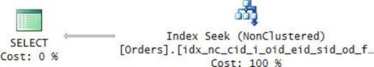
FIGURE 2-51 Plan that uses an index with included columns.
I got only 5 logical reads reported for this query.
When you’re done, run the following code for cleanup:
DROP INDEX dbo.Orders.idx_nc_cid_i_oid_eid_sid_od_flr;
Filtered indexes and statistics
A filtered index is an index on a subset of rows from the underlying table defined based on a predicate. You specify the predicate in a WHERE clause as part of the index definition. Filtered indexes are cheaper to create and maintain than nonfiltered ones because only modifications to the relevant subset of rows need to be reflected in the index. Also, filtered distribution statistics (histograms) are more accurate than nonfiltered statistics. That’s because the maximum number of steps in a histogram is 200, and with filtered statistics that number is used to represent a smaller set of rows. Furthermore, because the histogram is created on the leading key of the index only for the subset of rows that satisfy the index filter, effectively you get a quality of estimates as if you had a multicolumn histogram.
In cases where the index itself is not really important but statistics are, you can also create filtered statistics. You do so using the CREATE STATISTICS command, and specify the filter predicate in a WHERE clause.
As an example of a filtered index, suppose that you often query orders for the ship country USA and a certain order date period (since the beginning of the week, month, year). Perhaps you don’t issue similar queries for other ship countries as frequently. You need to speed up the queries specifically for the USA. You create an index with a filter based on the predicate shipcountry = N‘USA’ and specify the orderdate column as the key. If it’s important for you to avoid lookups, you will want to specify all remaining columns from the query as included columns. Run the following code to create such a filtered index:
USE TSQLV3;
CREATE NONCLUSTERED INDEX idx_USA_orderdate
ON Sales.Orders(orderdate)
INCLUDE(orderid, custid, requireddate)
WHERE shipcountry = N'USA';
Queries such as the following will then greatly benefit from the new index:
SELECT orderid, custid, orderdate, requireddate
FROM Sales.Orders
WHERE shipcountry = N'USA'
AND orderdate >= '20140101';
The execution plan for this query is shown in Figure 2-52.
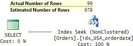
FIGURE 2-52 Plan with a filtered index and an inaccurate cardinality estimate.
Because the index filter matches the query filter, the optimizer considered the index as potentially useful. By the way, if the query filter is a subinterval of the index filter, the index can still be used. For example, if the index filter is col1 > 10 and the query filter is col1 > 20, the index can be used. Back to our example, because the index key column matches the column in the query’s range predicate, the optimizer could use a seek and a range scan to get the qualifying rows. Because the index covers the query, there was no need for lookups. The index is optimal for this query.
Curiously, despite what I said about the improved quality of cardinality estimates with filtered indexes, if you look at the query plan in Figure 2-52, the estimate doesn’t seem to be very accurate. In fact, it reflects the estimate for the filter based on the orderdate column alone. The thing is that here you’re not doing anything with the filtered rows, so the optimizer doesn’t really need a more accurate estimate. For example, if you add ORDER BY orderid to the query, you will see that the estimated number of rows coming out of the sort will be accurate.
An interesting tip I learned from Paul White is that if you add the filtered column (shipcountry in our case) to the index—for example, as an included column—the estimate will be based on the filtered statistics to begin with. With this in mind, re-create the index with shipcountry as an included column, like so:
CREATE NONCLUSTERED INDEX idx_USA_orderdate
ON Sales.Orders(orderdate)
INCLUDE(orderid, custid, requireddate, shipcountry)
WHERE shipcountry = N'USA'
WITH ( DROP_EXISTING = ON );
Rerun the query:
SELECT orderid, custid, orderdate, requireddate
FROM Sales.Orders
WHERE shipcountry = N'USA'
AND orderdate >= '20140101';
The execution plan for this query is shown in Figure 2-53.
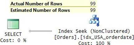
FIGURE 2-53 Plan with a filtered index and an accurate cardinality estimate.
Observe that this time the estimate is accurate.
You can also use filtered indexes to solve a common request related to enforcing data integrity. The UNIQUE constraint supported by SQL Server treats two NULLs as equal for the purposes of enforcing uniqueness. This means that if you define a UNIQUE constraint on a NULLable column, you are allowed only one row with a NULL in that column. In some cases, though, you might need to enforce the uniqueness only of non-NULL values but allow multiple NULLs. Standard SQL does support such a kind of UNIQUE constraint, but SQL Server never implemented it. With filtered indexes, it’s quite easy to handle this need. Simply create a unique filtered index based on a predicate in the form WHERE <column> IS NOT NULL. As an example, run the following code to create a table called T1 with such a filtered index on the column col1:
IF OBJECT_ID(N'dbo.T1', N'U') IS NOT NULL DROP TABLE dbo.T1;
CREATE TABLE dbo.T1(col1 INT NULL, col2 VARCHAR(10) NOT NULL);
GO
CREATE UNIQUE NONCLUSTERED INDEX idx_col1_notnull ON dbo.T1(col1) WHERE col1 IS NOT NULL;
Run the following code in an attempt to insert two rows with the same non-NULL col1 value:
INSERT INTO dbo.T1(col1, col2) VALUES(1, 'a'), (1, 'b');
The attempt fails with the following error:
Msg 2601, Level 14, State 1, Line 1023
Cannot insert duplicate key row in object 'dbo.T1' with unique index 'idx_col1_notnull'. The
duplicate key value is (1).
The statement has been terminated.
Try to insert two rows with a NULL in col1:
INSERT INTO dbo.T1(col1, col2) VALUES(NULL, 'c'), (NULL, 'd');
This time the code succeeds.
When you’re done, run the following code for cleanup:
USE TSQLV3;
DROP INDEX idx_USA_orderdate ON Sales.Orders;
DROP TABLE dbo.T1;
Columnstore indexes
Columnstore technology is a game changer in the database world. It was introduced initially in SQL Server 2012 and significantly improved in SQL Server 2014. This technology targets mainly data-warehousing workloads. Consider the classic star schema model for data warehouses as shown in Figure 2-54.
FIGURE 2-54 Star schema.
You have the dimension tables that keep track of the subjects you analyze the data by, like customers, employees, products, and time. Each dimension table has a surrogate key. The bulk of the data resides in the Fact table. This table has a column for the surrogate key of each of the dimension tables, plus columns representing measures like quantities and amounts. The traditional internal representation of the data in SQL Server before the introduction of columnstore technology has always been based on rowstore technology. This means that the data is stored and processed in a row-oriented mode. With the growing volume of data in data warehouses in recent years, rowstore technology tends to be inefficient on a number of levels, and columnstore technology addresses those inefficiencies.
To understand why rowstore is inefficient for large data warehouse environments, consider the typical data warehouse queries (also known as star join queries). They usually join the Fact table with some of the dimension tables, filter, group, and aggregate. Here’s an example of a typical data warehouse query in our PerformanceV3 database:
USE PerformanceV3;
SET STATISTICS IO, TIME ON; -- turn on performance statistics
SELECT D1.attr1 AS x, D2.attr1 AS y, D3.attr1 AS z,
COUNT(*) AS cnt, SUM(F.measure1) AS total
FROM dbo.Fact AS F
INNER JOIN dbo.Dim1 AS D1
ON F.key1 = D1.key1
INNER JOIN dbo.Dim2 AS D2
ON F.key2 = D2.key2
INNER JOIN dbo.Dim3 AS D3
ON F.key3 = D3.key3
WHERE D1.attr1 <= 10
AND D2.attr1 <= 15
AND D3.attr1 <= 10
GROUP BY D1.attr1, D2.attr1, D3.attr1;
The execution plan for this query is shown in Figure 2-55.
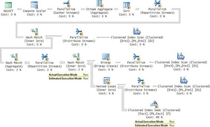
FIGURE 2-55 Plan for a star join query against a rowstore.
I got the following performance statistics for this query on my system:
Table 'Fact'. Scan count 122, logical reads 29300
CPU time = 890 ms, elapsed time = 490 ms.
The Fact table in the sample database has only 2,500,000 rows. Usually, data warehouses have much bigger tables. Our table is big enough, though, to justify a parallel plan and to allow me to illustrate the differences between rowstore and columnstore technologies. The bigger the tables are, the more advantageous it is to use columnstore technology, so keep in mind that in reality you will see much bigger differences than what you will see in my examples.
As mentioned, the rowstore technology has a number of drawbacks. There are so many possibilities in terms of indexing, causing you to spend a lot of time and energy on index tuning. If you have lots of query patterns in the system, it’s not going to be very practical for you to create the perfect covering index on the Fact table per query. You’ll end up with too many indexes. In an attempt to limit the number of indexes you create, you prioritize queries for tuning and also try to consolidate multiple queries with roughly similar indexing requirements. For example, if you have a number of queries that can benefit from indexes with the same key list but different include lists, you will probably prefer to create one index with a superset of the included columns. The result is that many queries won’t have truly optimal indexes to support them, and each query will likely end up using indexes that contain more than just the columns that are relevant to it. As you can realize, this means that queries will tend to perform more reads than the optimal number.
With rowstore, data is not compressed by default; rather, you need to explicitly request to compress it with row or page compression. Even if you do, because the data is stored a row at a time, the compression levels SQL Server can achieve are nowhere near what it can achieve with columnstore.
Another drawback of the rowstore technology is that currently the execution model for it is a row-execution model. This means that the different operators in the query plan are all limited to processing one row at a time. You can see this in the execution plan for our sample query in Figure 2-55. All operators in the plan will show the execution mode Row. (I highlighted this property for the clustered index seek against the Fact table and one of the hash joins.) A lot of CPU cycles are wasted because the operators process one row at a time. Any metadata information the operator needs to evaluate is evaluated per row. Any internal functions the operator needs to invoke are invoked per row.
Columnstore technology changes things quite dramatically. Note though that SQL Server 2012 is limited only to nonclustered, nonupdateable, columnstore indexes. SQL Server 2014 adds support for clustered, updateable indexes, making the technology much more accessible.
Use the following code to create a nonclustered columnstore index on our Fact table:
CREATE NONCLUSTERED COLUMNSTORE INDEX idx_nc_cs
ON dbo.Fact(key1, key2, key3, measure1, measure2, measure3, measure4);
You want to list all columns from the Fact table in the index. The order in which you list them isn’t significant. Unlike the key list in a rowstore index, which defines order, there is no similar concept of ordering in a columnstore index. Figure 2-56 illustrates how the data is organized in the columnstore index.
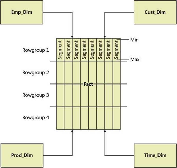
FIGURE 2-56 Columnstore applied to the Fact table.
SQL Server arranges the data in units called rowgroups. Each rowgroup has up to about 1,000,000 rows (more precisely, up to 220). You can find information about the rowgroups by querying the view sys.column_store_row_groups. Each rowgroup is split into the individual column segments, and each column segment is stored in a highly compressed form on a separate set of pages. You can find information about the column segments in the view sys.column_store_segments, including the minimum and maximum values in the column segment. SQL Server reduces storage requirements by using dictionaries that map entry numbers to the actual larger values. SQL Server always uses dictionaries for strings, and sometimes also for other types when there are few enough distinct values. You can find information about the dictionaries in the view sys.column_store_dictionaries.
Run our sample query again after creating the columnstore index:
SELECT D1.attr1 AS x, D2.attr1 AS y, D3.attr1 AS z,
COUNT(*) AS cnt, SUM(F.measure1) AS total
FROM dbo.Fact AS F
INNER JOIN dbo.Dim1 AS D1
ON F.key1 = D1.key1
INNER JOIN dbo.Dim2 AS D2
ON F.key2 = D2.key2
INNER JOIN dbo.Dim3 AS D3
ON F.key3 = D3.key3
WHERE D1.attr1 <= 10
AND D2.attr1 <= 15
AND D3.attr1 <= 10
GROUP BY D1.attr1, D2.attr1, D3.attr1;
The execution plan for this query is shown in Figure 2-57.
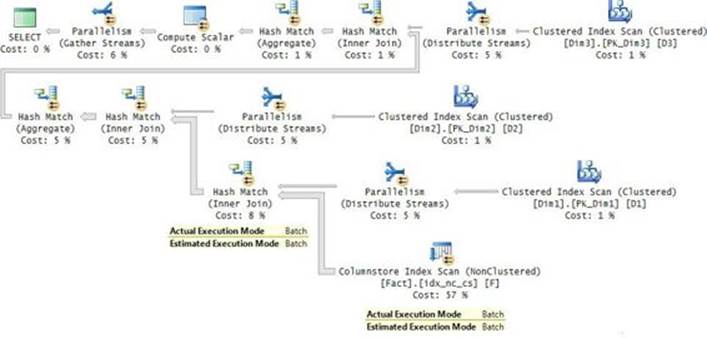
FIGURE 2-57 Plan for a star join query against a columnstore.
I got the following performance statistics for this query on my system:
Table 'Fact'. Scan count 8, logical reads 13235
CPU time = 172 ms, elapsed time = 185 ms.
As mentioned, our Fact table is pretty small in data warehousing terms. In practice, you will tend to work with much bigger tables and you will get much bigger performance differences between rowstore and columnstore.
One of the greatest things about the columnstore technology is that it pretty much eliminates the need to do index tuning on the Fact table. You just create one index. To fulfill a query, SQL Server constructs the result set only from the relevant columns. This is quite profound if you think about it; it’s as if you have all possible covering indexes without really needing to create a separate index for each case. Also, the fact that SQL Server constructs the result set only from the relevant columns tends to result in a significant reduction of I/O costs compared to rowstore.
Two other aspects of the columnstore technology tend to further reduce I/O costs. As mentioned, the level of compression that Microsoft managed to achieve with columnstore is much higher than with rowstore. Furthermore, remember that SQL Server records internally the minimum and maximum values of each column segment. If your query filters by a certain column, and the filtered values fall outside of the range covered by a column segment, the entire respective rowgroup is excluded. This capability is known as segment elimination.
An interesting aspect of the way the columnstore technology was implemented in SQL Server is that it is memory optimized, but it doesn’t require the entire data set to fit in memory. The columnstore technology also greatly benefits from parallel processing.
I described some aspects of the technology that tend to reduce I/O costs. There’s an aspect of the technology that tends to reduce CPU costs. Along with the columnstore technology, Microsoft introduced batch execution in SQL Server. A batch consists of a vectorized form of the relevant columns for a subset of the rows. Usually, the batch size is close to a thousand rows. Operators that were enhanced to support batch mode process a batch at a time instead of a row at a time. Internal functions that the operator executes use a batch as their input instead of a row. In the plan for our sample query, the operators that use batch mode are Columnstore Index Scan, all Hash operators, and the Compute Scalar operator. Figure 2-57 highlights two of the operators that use batch mode in this plan. Such operators will apply fewer iterations. Also, they evaluate the metadata information per batch instead of per row. All this translates to fewer CPU cycles. Currently, batch mode is used only when the data is organized as columnstore, but there’s nothing inherent in the technology that prevents it from being used also with rowstore. So perhaps we will see such support in the future.
As mentioned, support for columnstore in SQL Server 2012 was limited in a number of ways. You could create only a nonclustered columnstore index, which meant you had to create it in addition to the main rowstore-based representation of the data. With very large data warehouses, you have to consider the extra space requirements and the maintenance of two different representations of your data. The biggest limitation, though, is that once you create a nonclustered columnstore index, the table becomes nonupdateable. One way around this limitation is to maintain two tables with the same structure. One is a static partitioned table with a nonclustered columnstore index. Another is a trickle table without a columnstore index that absorbs the real-time changes. As soon as you are ready to make the trickle table part of the partitioned table, you create the nonclustered columnstore index on it, switch it into the partitioned table, and create a new trickle table to absorb the real-time changes. This solution also requires you to query both tables and unify the results.
The SQL Server 2012 implementation also has a number of limitations with the batch-execution feature. There’s a limited set of operators that support batch execution, and those that do, in some cases, will have to revert to row mode. For example, take the classic hash join algorithm, which is typically used in star join queries. The hash join operator can use batch execution only if the logical join type is an inner join; it always uses row mode with outer joins. Similarly, scalar aggregates are limited to row mode. In addition, if an operator doesn’t have enough memory and has to spill to tempdb, it switches to row mode. The process of switching from one mode to another is very static and can be done only at very specific points in the plan.
The SQL Server 2012 implementation is also more limited in its data type support with columnstore indexes. For example, it doesn’t support NUMERIC with a precision beyond 18, DATETIMEOFFSET with a precision beyond 2, BINARY, VARBINARY, UNIQUEIDENTIFIER, and others.
SQL Server 2014 has a number of significant improvements to the columnstore technology. The biggest one is support for clustered, updateable, columnstore indexes. Note, though, that if you create one, it cannot be unique, and you cannot create any other indexes on the table. As an example, the following code creates a table called FactCS with a clustered columnstore index and populates it with the rows from the table Fact:
CREATE TABLE dbo.FactCS
(
key1 INT NOT NULL,
key2 INT NOT NULL,
key3 INT NOT NULL,
measure1 INT NOT NULL,
measure2 INT NOT NULL,
measure3 INT NOT NULL,
measure4 NVARCHAR(50) NULL,
filler BINARY(100) NOT NULL DEFAULT (0x)
);
CREATE CLUSTERED COLUMNSTORE INDEX idx_cl_cs ON dbo.FactCS;
INSERT INTO dbo.FactCS WITH (TABLOCK) SELECT * FROM dbo.Fact;
When you use large-enough bulk inserts (102,400 rows or more) to add data to the table, SQL Server converts batches of up to 1,048,576 rows to columnstore format. When you perform nonbulk trickle inserts, SQL Server stores those in a rowgroup that uses a normal B-tree rowstore representation. Such a rowgroup is also known as a deltastore. As long as the deltastore keeps accepting new data, it will appear in the sys.column_store_row_groups view with the state description OPEN. Once the deltastore reaches the maximum size allowed for a rowgroup (1,048,576), it will stop accepting new data and SQL Server will mark it as CLOSED. A background process called tuple mover will then convert the data from the deltastore to the compressed columnstore format. When the process is done, the state of the rowgroup will appear as COMPRESSED.
SQL Server also supports deletes and updates. A delete of a row that resides in a deltastore is processed as a regular delete from a B-tree. A delete of a row from a compressed rowgroup causes the row ID of the deleted row to be written to a delete bitmap (an actual bitmap in memory and a B-tree on disk). When you query the data, SQL Server consults the delete bitmap to know which rows to consider as deleted. An update is handled as a delete followed by an insert.
The best thing about all this is that the query-processing layer is oblivious to this split between compressed rowgroups and deltastores; the storage-engine layer takes care of the details. This means that from the user’s perspective, it’s business as usual. The user submits reads and writes against the table, and behind the scenes the storage engine handles the writing to and reading from the deltastores and compressed rowgroups. One thing you do need to be aware of is that a large delete bitmap will slow down your queries. So, after a large number of deletes and updates, it would be a good idea to rebuild the table, like so:
ALTER TABLE dbo.FactCS REBUILD;
If the table is partitioned, you can rebuild the relevant partition by adding to the code PARTITION = <partition_number>.
SQL Server 2014 makes a number of improvements in batch-mode processing. For example, it can use batch mode in hash join operators that handle outer joins, in scalar aggregates, and in operators that spill to tempdb. It also handles cases where it needs to switch from one mode to another more dynamically. SQL Server 2014 also relaxes some of the restrictions related to data types. For example, it supports NUMERIC beyond precision 18, DATETIMEOFFSET beyond precision 2, BINARY and VARBINARY (although not with the MAX specifier), and UNIQUEIDENTIFIER.
Run the following star join query with the FactCS table this time:
SELECT D1.attr1 AS x, D2.attr1 AS y, D3.attr1 AS z,
COUNT(*) AS cnt, SUM(F.measure1) AS total
FROM dbo.FactCS AS F
INNER JOIN dbo.Dim1 AS D1
ON F.key1 = D1.key1
INNER JOIN dbo.Dim2 AS D2
ON F.key2 = D2.key2
INNER JOIN dbo.Dim3 AS D3
ON F.key3 = D3.key3
WHERE D1.attr1 <= 10
AND D2.attr1 <= 15
AND D3.attr1 <= 10
GROUP BY D1.attr1, D2.attr1, D3.attr1;
Note that the first time you run the query SQL Server will likely need to refresh existing statistics and create new ones, so the parse and compile time might take a bit longer. Run the query a second time to get a sense of the more typical run time. SQL Server reported the following performance statistics for this query on my system:
Table 'FactCS'. Scan count 8, logical reads 13556
CPU time = 139 ms, elapsed time = 219 ms.
For more information about the columnstore technology and the improvements in SQL Server 2014, see the following white paper: http://research.microsoft.com/apps/pubs/default.aspx?id=193599.
When you’re done, run the following code for cleanup:
SET STATISTICS IO OFF;
SET STATISTICS TIME OFF;
DROP INDEX idx_nc_cs ON dbo.Fact;
DROP TABLE dbo.FactCS;
Inline index definition
As you will learn in Chapter 10, SQL Server 2014 introduces support for memory-optimized tables as part of the In-Memory OLTP feature. In this first implementation, DDL changes are not allowed after the table creation. To allow you to define indexes on such tables as part of the table creation, Microsoft introduced syntax for inline index definition. Because Microsoft already made the effort mainly in the parser component, it extended the support for such a syntax also for disk-based tables, including table variables.
Remember that you cannot alter the definition of table variables once you declare them, so you cannot define indexes on existing table variables. Previously, you could define indexes only on table variables through PRIMARY KEY and UNIQUE constraints as part of the table definition, and therefore the indexes had to be unique. Now with the new inline index syntax, you can define nonunique indexes as part of the table variable definition, like so:
DECLARE @T1 AS TABLE
(
col1 INT NOT NULL
INDEX idx_cl_col1 CLUSTERED, -- column index
col2 INT NOT NULL,
col3 INT NOT NULL,
INDEX idx_nc_col2_col3 NONCLUSTERED (col2, col3) -- table index
);
Just like with constraints, you can define column-level indexes as part of a column definition and table-level indexes based on a composite key list as a separate item. Note that in the SQL Server 2014 implementation, inline indexes do not support the options UNIQUE, INCLUDE, and WHERE. For uniqueness, define the indexes like you used to indirectly through PRIMARY KEY or UNIQUE constraints.
Prioritizing queries for tuning with extended events
If you experience general performance problems in your system, besides trying to find and fix the bottlenecks, a common thing to do is to tune queries to be more efficient. The tricky part is that if you have lots of query patterns in the system, it’s not realistic to try and tune them all. You want to prioritize the queries for tuning so that you can spend more time on cases that, when tuned, will have a bigger impact on the system as a whole.
You need to decide which performance measure to use to prioritize the queries. It could be duration because that’s the user’s perception of performance. But it could also be that you identified a specific bottleneck in the system and need to rely on related measures. For example, if you identify a bottleneck in the I/O subsystem, you naturally will want to focus on I/O-related measures like writes and reads.
To measure query performance, you can capture a typical workload in your system using an Extended Events session with statement completed events. Remember that statement completed events carry performance information. For demonstration purposes, I’ll submit the sample workload with ad hoc queries from a specific SSMS session, so I’ll capture the sql_statement_completed event and filter by the session ID of the session in question. If the queries are submitted in your environment from stored procedures, you will need to capture the sp_statement_completedevent and apply any filters that are relevant to you.
A critical element that can help you prioritize which queries to tune is the query_hash action. It’s available to statement completed events starting with SQL Server 2012. This is a hash value that represents the template, or parameterized, form of the query string. Query strings that have the same template will get the same query hash value even if their input values are different. After you capture the workload, you group the events by the query hash value and order the groups (query templates) by the total relevant performance measure (say, duration in our example), descending. Then you spend more time and energy on the top templates.
Use the following code to create an Extended Events session that will capture the performance workload from the specified session into the specified target file (make sure to replace the session ID and file path with the ones relevant to you):
CREATE EVENT SESSION query_perf ON SERVER
ADD EVENT sqlserver.sp_statement_completed(
ACTION(sqlserver.query_hash)
WHERE (sqlserver.session_id=(54))),
ADD EVENT sqlserver.sql_statement_completed(
ACTION(sqlserver.query_hash)
WHERE (sqlserver.session_id=(54)))
ADD TARGET package0.event_file(SET filename=N'C:\Temp\query_perf.xel');
Use the following code to start the session:
ALTER EVENT SESSION query_perf ON SERVER STATE = START;
Assuming that the following set of queries represents your typical workload, run it a few times from the source SSMS session (54 in my case):
SELECT orderid, custid, empid, shipperid, orderdate
FROM dbo.Orders
WHERE orderid >= 1000000;
SELECT orderid, custid, empid, shipperid, orderdate
FROM dbo.Orders
WHERE custid = 'C0000000001';
SELECT orderid, custid, empid, shipperid, orderdate
FROM dbo.Orders
WHERE orderdate = '20140101';
SELECT orderid, custid, empid, shipperid, orderdate
FROM dbo.Orders
WHERE orderid >= 1000001;
SELECT orderid, custid, empid, shipperid, orderdate
FROM dbo.Orders
WHERE custid = 'C0000001000';
SELECT orderid, custid, empid, shipperid, orderdate
FROM dbo.Orders
WHERE orderdate = '20140201';
When you’re done running the workload, run the following code to stop the session:
ALTER EVENT SESSION query_perf ON SERVER STATE = STOP;
The event data was captured in the target file in XML format. Use the following code to copy the data from the file through the table function sys.fn_xe_file_target_read_file into a temporary table called #Events:
SELECT CAST(event_data AS XML) AS event_data_XML
INTO #Events
FROM sys.fn_xe_file_target_read_file('C:\Temp\query_perf*.xel', null, null, null) AS F;
Query the #Events table, and then extract the event columns from the XML using the value() method, placing them into a temporary table called #Queries, like so:
SELECT
event_data_XML.value ('(/event/action[@name=''query_hash'' ]/value)[1]', 'NUMERIC(38, 0)')
AS query_hash,
event_data_XML.value ('(/event/data [@name=''duration'' ]/value)[1]', 'BIGINT' )
AS duration,
event_data_XML.value ('(/event/data [@name=''cpu_time'' ]/value)[1]', 'BIGINT' )
AS cpu_time,
event_data_XML.value ('(/event/data [@name=''physical_reads'']/value)[1]', 'BIGINT' )
AS physical_reads,
event_data_XML.value ('(/event/data [@name=''logical_reads'' ]/value)[1]', 'BIGINT' )
AS logical_reads,
event_data_XML.value ('(/event/data [@name=''writes'' ]/value)[1]', 'BIGINT' )
AS writes,
event_data_XML.value ('(/event/data [@name=''row_count'' ]/value)[1]', 'BIGINT' )
AS row_count,
event_data_XML.value ('(/event/data [@name=''statement'' ]/value)[1]', 'NVARCHAR(4000)')
AS statement
INTO #Queries
FROM #Events;
CREATE CLUSTERED INDEX idx_cl_query_hash ON #Queries(query_hash);
You can now examine the query performance information conveniently by querying the #Queries table, like so:
SELECT query_hash, duration, cpu_time, physical_reads AS physreads,
logical_reads AS logreads, writes, row_count AS rowcnt, statement
FROM #Queries;
I got the following output on my system (the statement column is displayed on two lines to fit the printed page):
Query_hash duration cpu_time physreads logreads writes rowcnt statement
--------------------- --------- --------- ---------- --------- ------- ------- ----------------
3195161633580410947 234514 0 0 22 0 692 ... orderdate =
'20140101'
3195161633580410947 189375 0 0 21 0 671 ... orderdate =
'20140201'
...
14791727431994962596 272909 281000 0 4028 0 46 ... custid =
'C0000000001'
14791727431994962596 270893 281000 0 4016 0 42 ... custid =
'C0000001000'
...
15020196184001629514 405 0 0 6 0 1 ... orderid >=
1000000
15020196184001629514 354 0 0 3 0 0 ... orderid >=
1000001
...
Observe that queries that are based on the same template got the same query hash value even though their input values were different.
The final step is to issue a query against the table #Queries that groups the events by the query hash value and orders the groups by the sum of the desired performance measure (in this example, based on duration), descending, like so:
SELECT
query_hash, SUM(duration) AS sumduration,
CAST(100. * SUM(duration) / SUM(SUM(duration)) OVER() AS NUMERIC(5, 2)) AS pct,
(SELECT TOP (1) statement
FROM #Queries AS Q2
WHERE Q2.query_hash = Q1.query_hash) AS queryexample
FROM #Queries AS Q1
GROUP BY query_hash
ORDER BY SUM(duration) DESC;
I got the following output on my system:
query_hash sumduration pct queryexample
--------------------- ------------ ------ ----------------------------------------------------
14791727431994962596 3159476 58.13 SELECT orderid, custid, empid, shipperid, orderdate
FROM dbo.Orders
WHERE custid = 'C0000000001'
3195161633580410947 2267599 41.72 SELECT orderid, custid, empid, shipperid, orderdate
FROM dbo.Orders
WHERE orderdate = '20140101'
15020196184001629514 7963 0.15 SELECT orderid, custid, empid, shipperid, orderdate
FROM dbo.Orders
WHERE orderid >= 1000001
I had only three query templates in my sample workload. Naturally, in an active system you will have many more. At this point, you know which queries are more important to tune in terms of the potential effect on the system as a whole.
When you’re done, drop the temporary tables and the Extended Events session by running the following code:
DROP TABLE #Events, #Queries;
DROP EVENT SESSION query_perf ON SERVER;
Index and query information and statistics
SQL Server provides you with a wealth of performance-related information about your indexes and queries through dynamic management views (DMVs) and dynamic management functions (DMFs). This section describes some objects I find particularly useful.
Earlier in the chapter, I discussed index fragmentation. You can query the sys.dm_db_index_physical_stats function to get physical statistics about your indexes, including fragmentation levels. For example, the following code returns information about all indexes in the PerformanceV3 database (the NULLs stand for all tables, all indexes, and all partitions):
SELECT database_id, object_id, index_id, partition_number,
avg_fragmentation_in_percent, avg_page_space_used_in_percent
FROM sys.dm_db_index_physical_stats( DB_ID('PerformanceV3'), NULL, NULL, NULL, 'SAMPLED' );
To evaluate fragmentation, I examine two measures: avg_fragmentation_in_percent is the percentage of out-of-order pages (also known as logical scan fragmentation), and avg_page_space_used_in_percent is the average page population expressed as a percentage.
You want to be careful when you run such code in a production environment because the information is actually gathered when you query this object. The DETAILED mode is the most expensive one because it involves full scans of the data. The LIMITED mode is the cheapest because it examines only parent index pages (nonleaf), but for this reason it cannot report the average page population. The SAMPLED mode scans one percent of the data, and therefore is a good compromise between the two.
When you have a high level of logical scan fragmentation and you find that it negatively affects your query performance, the remedy is to rebuild or reorganize the index. Similarly, if you have too much free space, or too little (which results in splits), you rebuild the index and, if relevant, specify the desired fill factor.
Use ALTER INDEX REBUILD to rebuild the index, like so:
ALTER INDEX <index_name> ON <table_name> REBUILD WITH (FILLFACTOR = 70 /*, ONLINE = ON */);
Use ALTER INDEX REORGANIZE to reorganize the index, like so:
ALTER INDEX <index_name> ON <table_name> REORGANIZE;
The REBUILD option allows specifying a fill factor, and its result tends to be more effective than the REORGANIZE option; however, the former is an offline operation, whereas the latter is an online one. You can rebuild an index as a mostly online operation if you’re using the Enterprise edition of SQL Server by adding the ONLINE = ON option; however, an online rebuild is a longer and more expensive operation, so you better do it as an offline one if you can allow some downtime.
You need to be able to identify which indexes are used more often and which are rarely or never used. You don’t want to keep indexes that are rarely used, because they do have a negative performance effect on modifications. SQL Server collects index-usage information in the background and enables you to query it through dynamic management objects called dm_db_index_operational_stats and dm_db_index_usage_stats. The dm_db_index_operational_stats function gives you low-level I/O, locking, latching, and access-method activity information. For example, to get information about all objects, indexes, and partitions in the PerformanceV3 database, you query the function like so:
SELECT * FROM sys.dm_db_index_operational_stats( DB_ID('PerformanceV3'), null, null, null );
The dm_db_index_usage_stats view gives you usage counts of the different access methods (scan, seek, lookup):
SELECT * FROM sys.dm_db_index_usage_stats;
Recall from earlier examples, such as in Figure 2-31, that in some plans SQL Server identifies missing indexes. SQL Server also records such missing index information internally and exposes it through the dynamic management objects sys.dm_db_missing_index_details,sys.dm_db_missing_index_group_stats, sys.dm_db_missing_index_groups, and sys.dm_db_missing_index_columns. Query those objects to get missing index information that was collected since SQL Server was last restarted.
The sys.dm_db_missing_index_details view contains most of the interesting information. Run the following code to query the view in your system:
SELECT * FROM sys.dm_db_missing_index_details;
This view has a row for each missing index. The attributes equality_columns and inequality_columns report the columns that are candidates as key columns in the index. The included_columns attribute reports the columns that are candidates as included columns in the index if it’s important for you to avoid lookups.
Make sure, though, that you apply your knowledge, your experience, and some common sense in choosing which recommendations to follow. You might find redundant recommendations. For example, if two queries look the same but only slightly differ in the returned set of columns (for example, one returns col1 and col2 and the other returns col1 and col3), you will get different missing index recommendations. You can easily consolidate such recommendations and create one index with the superset of included columns (col1, col2, and col3).
The view sys.dm_db_missing_index_group_stats gives you summary statistics about groups of missing indexes, like the average user impact. At the moment, an index group contains only one index. Perhaps the thinking was to allow the future arrangement of multiple indexes in groups. Run the following code to query the view in your system:
SELECT * FROM sys.dm_db_missing_index_group_stats;
The view sys.dm_db_missing_index_groups gives you a group-to-index connection (again, at the moment, it is a one-to-one relationship). Use the following code to query the view in your system:
SELECT * FROM sys.dm_db_missing_index_groups;
Query the sys.dm_db_missing_index_columns function with a specific index handle you obtain from the sys.dm_db_missing_index_details view to get information about the columns of the missing index individually. The result will tell you if the column role is equality or inequality. Such information can help you determine which columns to specify in the index key list and which to specify in the include list. Query the function like so:
SELECT * FROM sys.dm_db_missing_index_columns(<handle>);
SQL Server supports a handy view called sys.dm_exec_query_stats that aggregates query performance information for queries whose plans are in cache. Querying such a view is so much easier than working with an Extended Events session to get query performance information, but keep in mind that this view won’t report information for queries whose plans are not in cache. The information that this view provides for each cached query plan includes, among other things, the following:
![]() A SQL handle that you can provide as input to the function sys.dm_exec_sql_text to get the text of the parent query or batch of the current query. You also get the start and end offsets of the query that the current row represents so that you can extract it from the full parent query or batch text. Note that the offsets are zero based and are specified in bytes, although the text is Unicode (meaning two bytes of storage per character).
A SQL handle that you can provide as input to the function sys.dm_exec_sql_text to get the text of the parent query or batch of the current query. You also get the start and end offsets of the query that the current row represents so that you can extract it from the full parent query or batch text. Note that the offsets are zero based and are specified in bytes, although the text is Unicode (meaning two bytes of storage per character).
![]() A plan handle that you can provide as input to the function sys.dm_exec_query_plan to get the XML form of the plan.
A plan handle that you can provide as input to the function sys.dm_exec_query_plan to get the XML form of the plan.
![]() The creation time and last execution time.
The creation time and last execution time.
![]() The execution count.
The execution count.
![]() Performance information, including worker (CPU) time, physical reads, logical reads, CLR time, and elapsed time. For each performance counter, you get the total for all invocations of the plan: last, minimum, and maximum.
Performance information, including worker (CPU) time, physical reads, logical reads, CLR time, and elapsed time. For each performance counter, you get the total for all invocations of the plan: last, minimum, and maximum.
![]() Query hash and plan hash values. You use the former to identify queries with the same query template (similar to the query_hash action in Extended Events). With the latter, you can identify similar query execution plans.
Query hash and plan hash values. You use the former to identify queries with the same query template (similar to the query_hash action in Extended Events). With the latter, you can identify similar query execution plans.
![]() Row counts.
Row counts.
Run the following code to query the view in your system:
SELECT * FROM sys.dm_exec_query_stats;
If you want to isolate top query templates that represent more work, you can group the data in the view by the query_hash attribute, and order the groups by the sum of the performance measure of interest, descending, like so (using duration in this example):
SELECT TOP (5)
MAX(query) AS sample_query,
SUM(execution_count) AS cnt,
SUM(total_worker_time) AS cpu,
SUM(total_physical_reads) AS reads,
SUM(total_logical_reads) AS logical_reads,
SUM(total_elapsed_time) AS duration
FROM (SELECT
QS.*,
SUBSTRING(ST.text, (QS.statement_start_offset/2) + 1,
((CASE statement_end_offset
WHEN -1 THEN DATALENGTH(ST.text)
ELSE QS.statement_end_offset END
- QS.statement_start_offset)/2) + 1
) AS query
FROM sys.dm_exec_query_stats AS QS
CROSS APPLY sys.dm_exec_sql_text(QS.sql_handle) AS ST
CROSS APPLY sys.dm_exec_plan_attributes(QS.plan_handle) AS PA
WHERE PA.attribute = 'dbid'
AND PA.value = DB_ID('PerformanceV3')) AS D
GROUP BY query_hash
ORDER BY duration DESC;
This query generated the following output on my system:
sample_query cnt cpu reads logical_reads duration
---------------------------------------- ---- -------- ------ -------------- ---------
SELECT ... WHERE custid = 'C0000001000' 10 3155513 92 40305 3158897
SELECT ... FROM dbo.FactCS AS F 8 2021766 1 110332 2929692
SELECT ... WHERE orderid <= 100000 1 463615 0 25339 2805217
SELECT ... WHERE orderdate = '20140201' 10 15054 0 215 2266620
SELECT ... WHERE custid LIKE '%9999' 1 1828461 0 4283 1887095
SQL Server provides you with similar views called sys.dm_exec_procedure_stats and sys.dm_exec_trigger_stats to query procedure and trigger performance statistics. Run the following code to query these views in your system:
SELECT * FROM sys.dm_exec_procedure_stats;
SELECT * FROM sys.dm_exec_trigger_stats;
SQL Server 2014 introduces a curious new DMV called sys.dm_exec_query_profiles. This view provides real-time query plan progress. It returns a row for every operator in an active actual query plan or, more precisely, for every operator and thread in the plan, with progress information. It shows the estimated row count as well as the actual row count produced so far, I/O, CPU and elapsed time information, open and close times, first and last times the operator was active, first and last times it produced a row, and more. It’s a supercool feature. Note, though, that you need to have some form of an actual query plan enabled for the view to report information about the plan. To achieve this, you can enable the Include Actual Execution Plan option in SSMS, turn on the STATISTICS PROFILE or STATISTICS XML session options, run an Extended Events session with the event query_post_execution_showplan, or a trace with the events Showplan Statistics Profile or Showplan XML Statistics Profile.
As an example, enable the Include Actual Execution Plan option in SSMS and run the following expensive query:
SELECT O1.orderid, O1.orderdate, MAX(O2.orderdate) AS mxdate
FROM dbo.Orders AS O1
INNER JOIN dbo.Orders AS O2
ON O2.orderid <= O1.orderid
GROUP BY O1.orderid, O1.orderdate;
To see the live query progress, query the view in a different query pane, like so:
SELECT * FROM sys.dm_exec_query_profiles;
I’m just waiting for some company like SQL Sentry, which developed the popular Plan Explorer tool, to come forward and, based on the information in the view, provide a graphical animated view of the real-time progress of a query plan. Who knows, perhaps by the time you read these words some company will have already done this.
Temporary objects
This section covers the use of temporary tables and table variables as tools to aid in query tuning. These objects are often misunderstood, and this misunderstanding tends to lead to suboptimal solutions. Hopefully, with the information in this section you will be equipped with correct understanding of these objects, and will use them efficiently. I’ll refer to temporary tables and table variables collectively as temporary objects.
Temporary objects are used for various purposes, not just performance related. For example, you need such objects when you have a process that requires you to set aside intermediate result sets for further processing. Because the focus of this chapter is query tuning, I’ll discuss the use of such objects mainly for query tuning purposes.
In a number of cases, you’ll find it beneficial to use temporary objects from a query-tuning perspective. One case is when you have an expensive query that generates a small result set and you need to refer to this result set multiple times. Naturally, you want to avoid repeating the work. Another case is to help improve cardinality estimates. SQL Server uses statistics to make cardinality estimates mainly in the leaf nodes of the plan, but the farther the data flows in the plan, the more likely it is that the quality of cardinality estimates will degrade. If you have a query that involves a lot of tables and a lot of manipulation, and you observe suboptimal choices in the plan that you connect to inaccurate cardinality estimates, one way to deal with those is to split the original solution into steps. Extract the part of the work, like a subset of the joins, up to the point where you see the problem in the plan, and write the result to a temporary object. Then apply the next step between the temporary object and the rest of the tables. This will give the optimizer a fresh start and, I hope, lead to a more efficient solution overall.
In the upcoming sections, I compare and contrast the different types of temporary objects that SQL Server supports. I compare local temporary tables (named with a number sign as prefix, as in #MyTable), table variables (named with the at sign as prefix, as in @MyTable), and table expressions such as derived tables and CTEs. For reference purposes, Table 2-2 has a summary of the comparison.
TABLE 2-2 Temporary objects
There are a number of common misconceptions concerning the use of temporary objects. Probably the oldest one is that some people incorrectly believe that table variables reside only in memory and have no disk-based representation. The source for this misconception is probably that people intuitively think that a variable is always a memory-only resident object. The reality is that temporary tables and table variables are represented the same way as a set of pages in tempdb and can incur disk activity.
Interestingly, the technology seems to be catching up with the misconception. Certain improvements in recent versions of SQL Server could result in reduced activity or no disk activity. For example, starting with SQL Server 2014 you can define a table type as a memory-optimized one (using the MEMORY_OPTIMIZED = ON option). Then, when you declare a table variable of this type, it is represented as a memory-optimized table. This feature is part of the In-Memory OLTP engine and is described in Chapter 10.
Another improvement in SQL Server 2014 (also backported to SQL Server 2012) is related to how SQL Server handles what’s called eager writes for bulk operations like SELECT INTO in tempdb. Normally, eager writes eagerly flush dirty pages associated with bulk operations to disk to prevent such operations from flooding the memory with new pages. With the new feature, when you perform bulk operations in tempdb, the eager-writing behavior is relaxed, not forcing the flushing of dirty pages as quickly as before. This improvement can be beneficial when you create and populate a temporary object with a bulk operation, query it, and drop it quickly. Now such work can be done with reduced activity or no disk activity.
Another common misconception concerns table expressions like derived tables and CTEs. Some intuitively think that when you use a table expression, SQL Server persists the inner query’s result in a work table if it is beneficial to do so from a performance perspective. Theoretically, such potential exists, but the reality is that, so far, Microsoft has not introduced such a capability to the engine. Any reference to a table expression gets unnested (inlined), and the query plan interacts with the underlying objects directly. This fact is especially important to remember when you have an expensive query and you need to interact with its result set multiple times—perhaps even with the same query. All references to the table expression will be inlined, and the expensive work will be repeated. It’s easy to demonstrate this behavior. Start by running the following code to enable reporting performance statistics:
SET STATISTICS IO, TIME ON;
Consider the following query, which computes yearly order counts:
SELECT YEAR(orderdate) AS orderyear, COUNT(*) AS numorders
FROM dbo.Orders
GROUP BY YEAR(orderdate);
I got the following performance statistics for this query on my system: logical reads = 2,641, CPU time = 861 ms, elapsed time = 289 ms.
You need to come up with a solution that, for each current year, returns the year with the closest count of orders and the difference between the order counts between the two years. To achieve this, you use the following query (if you’re not familiar with the CROSS APPLY operator, you can find details in Chapter 3):
WITH C AS
(
SELECT YEAR(orderdate) AS orderyear, COUNT(*) AS numorders
FROM dbo.Orders
GROUP BY YEAR(orderdate)
)
SELECT C1.orderyear, C1.numorders,
A.orderyear AS otheryear, C1.numorders - A.numorders AS diff
FROM C AS C1 CROSS APPLY
(SELECT TOP (1) C2.orderyear, C2.numorders
FROM C AS C2
WHERE C2.orderyear <> C1.orderyear
ORDER BY ABS(C1.numorders - C2.numorders)) AS A
ORDER BY C1.orderyear;
Examine the query plan for this query as shown in Figure 2-58.
FIGURE 2-58 Query plan with a CTE shows the expensive work is repeated.
The middle branch in the plan (outer input of the Nested Loops operator) represents the instance of the CTE called C1, which is referenced in the FROM clause of the outer query. It involves scanning, grouping, and aggregating the data from the Orders table once. The bottom branch in the plan (the inner input of the Nested Loops operator) represents the instance of the CTE called C2, which is referenced by the TOP (1) subquery. This branch also involves scanning, grouping, and aggregating the data from the Orders table. Because there are five years currently in the outer table C1, this branch is activated five times. In total, the expensive work was repeated six times. I got the following performance statistics from this query: logical reads = 15,696 (6 scans), CPU time = 4763 ms, elapsed time = 1938 ms.
To avoid repeating the expensive work, you should persist the result of the grouped query in a temporary table or a table variable. Here’s an example of how you can achieve this using a table variable:
DECLARE @T AS TABLE
(
orderyear INT,
numorders INT
);
INSERT INTO @T(orderyear, numorders)
SELECT YEAR(orderdate) AS orderyear, COUNT(*) AS numorders
FROM dbo.Orders
GROUP BY YEAR(orderdate)
SELECT T1.orderyear, T1.numorders,
A.orderyear AS otheryear, T1.numorders - A.numorders AS diff
FROM @T AS T1 CROSS APPLY
(SELECT TOP (1) T2.orderyear, T2.numorders
FROM @T AS T2
WHERE T2.orderyear <> T1.orderyear
ORDER BY ABS(T1.numorders - T2.numorders)) AS A
ORDER BY T1.orderyear;
The execution plans for these statements are shown in Figure 2-59.
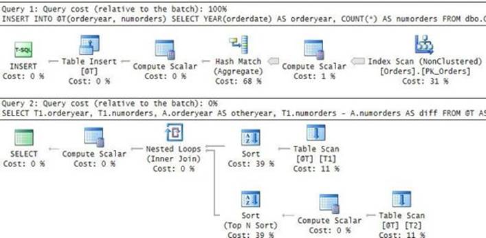
FIGURE 2-59 Query plan with a table variable shows the expensive work is not repeated.
The first execution plan is for the code that computes the yearly aggregates and writes those to the table variable. Observe that 100 percent of the cost of the batch (in reality it’s almost 100 percent) is associated with this activity. The second execution plan is for the query against the table variable. The important thing here is that this solution executes the bulk of the work only once. The table variable is accessed six times by the second query, but it’s so tiny that this part of the work is negligible. Here are the performance statistics I got for this solution: logical reads = 2,622, CPU time = 468 ms, elapsed time = 572 ms. That’s one-sixth of the reads and less than one-third of the run time of the solution with the CTE. In short, remember that table expressions don’t have a physical side to them; they don’t get persisted anywhere. When you query them, SQL Server translates the work directly to the underlying objects. If you need to persist the result somewhere, you should be using temporary tables or table variables.
The key difference between temporary tables and table variables from a performance perspective is in the kinds of statistics that SQL Server maintains for each. SQL Server maintains the same types of statistics for temporary tables that it does for permanent ones. This includes the statistics header, density vectors, and histogram. For table variables, SQL Server maintains only the table’s cardinality, and even this limited information is typically not visible to the optimizer, as I will demonstrate shortly. Theoretically, because temporary tables have more statistics, queries involving them should get more accurate cardinality estimates, and therefore more optimal plans than table variables. In some cases, that’s what you will experience. But you know what Einstein said about theory and practice: “In theory, theory and practice are the same. In practice, they are not.” You should be aware that especially when using temporary tables in stored procedures, certain complications can lead to inaccurate estimates. I’ll elaborate on this point later. Pro tem, for simplicity’s sake, assume that with temporary tables, because of the existence of more statistics, you will tend to get better plans than with table variables.
If you tend to get better plans with temporary tables, why even bother with table variables? There are both performance reasons and logical ones. From a performance standpoint, because table variables don’t have statistics, you don’t pay the costs related to creating and maintaining those. Furthermore, you will tend to get fewer recompilations. If you think about it, when the volume of data you need to store in the temporary object is very small (just a few pages), you don’t really care much about the accuracy of the estimates. Then you might as well use table variables and benefit from the fewer recompiles. Such is the case with our last solution. When working with data beyond just a few pages, you will typically care about the quality of the estimates, and the cost of maintaining statistics and the related recompilations associated with temporary tables will typically be worth it.
I mentioned that the table cardinality is recorded for table variables but that often it’s not visible to the optimizer. This has much to do with the earlier discussion about cardinality estimates when variables are involved. I explained that because the initial optimization unit is the batch and not the statement, normally the optimizer cannot sniff variable values. The same applies to table variables. If the same batch declares, populates, and queries the table variable, the optimizer gets to optimize the query before the table variable is populated. So it cannot know what the cardinality of the table is. Like with regular variables, if you add the RECOMPILE query option, the query will get optimized after the table variable is populated; therefore, its cardinality will be visible to the optimizer. But this will cost you a recompile every time you execute the code. Another option to make the table cardinality visible is to pass the table variable as a table-valued parameter to a stored procedure, and this way get parameter sniffing.
I’ll use the following code and the related query plans to demonstrate cardinality estimates with table variables:
DECLARE @T AS TABLE
(
col1 INT NOT NULL PRIMARY KEY NONCLUSTERED,
col2 INT NOT NULL,
filler CHAR(200) NOT NULL
);
INSERT INTO @T(col1, col2, filler)
SELECT n AS col1, n AS col2, 'a' AS filler
FROM TSQLV3.dbo.GetNums(1, 100000) AS Nums;
-- Query 1
SELECT col1, col2, filler
FROM @T
WHERE col1 <= 100
ORDER BY col2;
-- Query 2
SELECT col1, col2, filler
FROM @T
WHERE col1 <= 100
ORDER BY col2
OPTION(RECOMPILE);
-- Query 3
SELECT col1, col2, filler
FROM @T
WHERE col1 >= 100
ORDER BY col2
OPTION(RECOMPILE);
The execution plans for these three queries are shown in Figure 2-60.
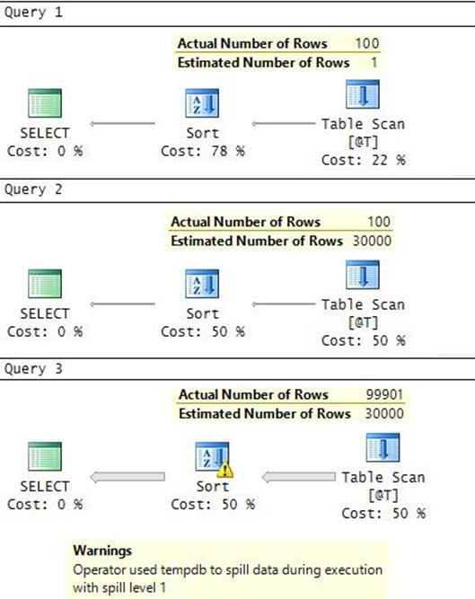
FIGURE 2-60 Query plans with a table variable.
The code declares a table variable called @T with three columns called col1, col2, and filler, with a nonclustered index called PK_T1 defined on col1. The code populates the table variable with 100,000 rows. The code then issues three queries. Query 1 filters the rows where col1 <= 100. Query 2 filters the rows where col1 <= 100 and has the RECOMPILE option. Query 3 filters the rows where col1 >= 100 and has the RECOMPILE option. All queries order the result rows by col2. The index PK_T1 can support the query filters, but because it’s not a covering index, if the optimizer decides to use it, lookups will be involved. Because the first two queries are very selective, they would benefit from a plan that uses the index and applies a few lookups. The last query is nonselective and would benefit from a scan.
Looking at the plans in Figure 2-60, you see inefficient choices in all three plans. In the first plan, the optimizer doesn’t have the table cardinality available, so it assumes that it’s very small. As a result, it uses a scan. In the second plan, thanks to the RECOMPILE query option, the optimizer does have the table cardinality available; however, because there’s no histogram available and you used the <= operator, it estimates 30% matches. (Remember the magic table of estimates in Table 2-1?) In the third plan—again, thanks to the RECOMPILE query option—the optimizer does have the table cardinality available, and also here the estimate is 30% because you used the operator >=. However, in this case, 30% is an underestimate, which results in a spill of the sort operation to tempdb.
Another option to make the cardinality of a table variable visible is to use trace flag 2453, which is available in SQL Server 2014 RTM CU3 and later and in SQL Server 2012 SP2 and later. This trace flag causes SQL Server to trigger recompiles based on the same thresholds that it uses for normal tables. This means that instead of forcing a recompile explicitly in every execution of the query, you will get fewer automated recompiles. When an automated recompile does happen, the table cardinality becomes available. You can find details about this trace flag here:http://support.microsoft.com/kb/2952444/en-us.
With temporary tables, you will tend to get better cardinality estimates and, consequently, better plans, as the following code demonstrates:
CREATE TABLE #T
(
col1 INT NOT NULL PRIMARY KEY NONCLUSTERED,
col2 INT NOT NULL,
filler CHAR(200) NOT NULL
);
INSERT INTO #T(col1, col2, filler)
SELECT n AS col1, n AS col2, 'a' AS filler
FROM TSQLV3.dbo.GetNums(1, 100000) AS Nums
OPTION(MAXDOP 1);
GO
-- Query 1
SELECT col1, col2, filler
FROM #T
WHERE col1 <= 100
ORDER BY col2;
-- Query 2
SELECT col1, col2, filler
FROM #T
WHERE col1 >= 100
ORDER BY col2;
GO
-- Cleanup
DROP TABLE #T;
The execution plans for the two queries are shown in Figure 2-61.
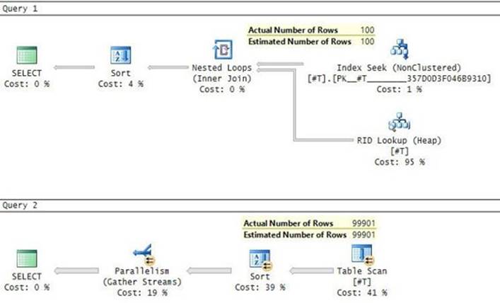
FIGURE 2-61 Query plans with a temporary table.
You can see in the plans that the cardinality estimates are accurate. As expected, the plan for the first query performs a seek and lookups. The plan for the second query is a parallel plan that performs a scan, and the sort doesn’t spill to tempdb.
I mentioned that in theory queries involving temporary tables should get better cardinality estimates, but that in practice things are not always that simple. The complications have to do with a certain caching mechanism SQL Server uses for temporary tables, table variables, and worktables SQL Server creates as part of the query plan. Recall from the discussions about the internal data structures earlier in the book that, by default, the first eight page allocations for a new table are done from mixed extents. Also remember that SQL Server uses SGAM pages to map the extents in the file that are mixed and have a page available for allocation. Temporary objects start empty, and the first few allocations for those will tend to be single-page allocations from mixed extents. Every time your modification allocates a page from a mixed extent, it needs to obtain an update latch on the respective SGAM page. As you can realize, with many temporary objects created at the same time, the situation can potentially lead to a bottleneck as a result of page-latch contention against the SGAM pages.
SQL Server has an internal caching mechanism designed to reduce such contention. Say that you execute a stored procedure where you use a temporary table or a table variable. When the procedure finishes, the temporary object is normally supposed to be destroyed. With this caching mechanism, SQL Server keeps some resources of the temporary object in cache. Those include the metadata entries, one IAM page, and one data page. The next time you (or someone else) execute the stored procedure, if such resources are available in cache, SQL Server can connect your new logical temporary object to those cached physical resources. By doing so, some page allocations are avoided and, thus, contention is reduced.
All this sounds nice in theory. In practice, there’s a small problem; apparently, SQL Server also caches and reuses the statistics for those temporary objects. The odd thing is that the internal modification counter of changes in the temporary objects, which SQL Server uses to know whetherto trigger a refresh of the statistics, accumulates across procedure calls. Consequently, if SQL Server optimizes a query against a temporary object in a stored procedure and the recompilation threshold wasn’t reached yet, it might end up using distribution information that was created earlier for a different execution of the procedure. You must be thinking, “No way!” Well, I’m afraid it’s “Yes way!” Enough said by me. I cannot do this topic as good a service as Paul White did with the following two brilliant articles:
![]() http://sqlblog.com/blogs/paul_white/archive/2012/08/15/temporary-tables-in-stored-procedures.aspx
http://sqlblog.com/blogs/paul_white/archive/2012/08/15/temporary-tables-in-stored-procedures.aspx
![]() http://sqlblog.com/blogs/paul_white/archive/2012/08/17/temporary-object-caching-explained.aspx
http://sqlblog.com/blogs/paul_white/archive/2012/08/17/temporary-object-caching-explained.aspx
Not only is the information in these articles gold, the articles are also a sheer pleasure to read.
Paul’s recommendation is that in those targeted cases where you find the problem, you can explicitly update statistics in the temporary table right before the query and add the RECOMPILE option to the query. This will trigger a refresh of the statistics and a recompile.
Back to the discussion about the differences between temporary tables and table variables: another difference is in scope and visibility. Like regular variables, a table variable is visible only to the batch that declared it. A local temporary table is visible only to the session that created it, including the entire level in which it was created as well as all inner levels in the call stack. It gets automatically destroyed (logically, at least) as soon as the level that created it goes out of scope. With ad hoc code, this means that the temporary table will even be able to cross batch boundaries. With stored procedures and triggers, as soon as the module that created the temporary table terminates, the temporary table is destroyed. This means that if you create a temporary table in one level, you will be able to interact with it in inner levels like an inner procedure, trigger, or dynamic batch. If your scope requirements dictate that the temporary object should be visible in an inner level in the call stack, you will have to use a temporary table. If you create a global temporary table (with two number signs as a prefix, as in ##MyTable), it’s visible globally (not just to the session that created it) and destroyed as soon as the session that created it terminates and there are no active references.
Another curious difference between temporary tables and table variables is what happens when you modify them in a transaction that eventually rolls back. In such a case, changes against a temporary table are undone just like changes against a permanent table. But with table variables, only a single-statement change that doesn’t complete is undone. As soon as a single-statement change completes, the changes survive a rollback. This capability of table variables makes them extremely useful in transactions and triggers that fail (or when you fail them) and where you need to keep information created by the transaction. For example, suppose that you make changes in a transaction within a TRY block. If the transaction fails, it enters a doomed state and control is passed to the CATCH block. You have to roll back the doomed transaction. But what if there’s critical information that the transaction generated and you need to save. The trick is to copy the data you need to save into table variables in the CATCH block and then roll back the transaction. The data in the table variables survives the rollback, and you can then save it wherever you need in a new transaction.
In a similar manner, suppose that you have a trigger and, in certain conditions, you need to issue a rollback from the trigger. But you need to save the information from the inserted and deleted tables. If you issue a rollback, all data in inserted and deleted disappears. If you first copy the data from inserted and deleted to the target tables and then do the rollback, the copying to the target tables will be undone too. The solution is that before you issue the rollback, you copy the data from inserted and deleted into table variables. You then issue a rollback, and after the rollback you copy the data from the table variables to the target tables.
Set-based vs. iterative solutions
One of the common dilemmas people have when they need to solve a querying task is whether to use a set-based approach or an iterative one in their solution. The relational model is based, in part, on mathematical set theory. You solve a task using a set-based approach by applying principles that are based on set theory. Here’s the definition of a set as formulated by Georg Cantor—the creator of set theory:
By a “set” we mean any collection M into a whole of definite, distinct objects m (which are called the “elements” of M) of our perception or of our thought.
—Joseph W. Dauben, Georg Cantor (Princeton University Press, 1990)
To me, a set-based solution interacts with an input table as a whole, and it doesn’t make any assumptions about the physical order of the data in terms of the correctness of the solution. You can implement such solutions with T-SQL queries without iterations. Conversely, an iterative solution manipulates one row at a time and can rely on the order of the data. You can manipulate one row at a time using a cursor mechanism or a loop with TOP (1) queries.
There are two main reasons why I generally prefer to use the set-based approach as my default and consider the iterative approach only in exceptional cases. One reason is philosophical, and the other is pragmatic. The philosophical dimension is that I feel that an approach based on strong mathematical foundations is likely going to result in more stable and robust solutions. The relational model survived so many years probably because it is based on strong mathematical foundations, unlike so many other aspects of computing that are based more on intuition and tend to be shorter lasting.
The pragmatic dimension is that iterative constructs in T-SQL are very inefficient compared to iterative constructs in many other programming languages. For example, the T-SQL WHILE loop is much slower than a while loop in C#. Similarly, working with a T-SQL cursor is much slower than working with the SQLDataReader object in .NET. So T-SQL set-based solutions tend to perform better than T-SQL iterative ones.
Interestingly, the execution model SQL Server uses when it executes a query plan for a T-SQL set-based solution is, after all, iterative. When SQL Server executes a query plan, the various operators perform iterations (hence, they are also known as iterators) to process one row at a time. But the language that SQL Server uses to perform those iterations isn’t T-SQL; rather, it is some low-level language that is highly efficient in applying them.
I consider iterative solutions in exceptional cases where the optimizer doesn’t do a good job at optimizing my set-based solution and I feel that I exhausted my tuning options. But then, I can get much better performance by implementing a CLR-based iterative solution rather than a T-SQL-based one.
To demonstrate how expensive a T-SQL iterative solution can be compared to a set-based one, I’ll use a task such as grouping and aggregating as my example. To make the problem a bit more interesting than just a basic grouping problem, I’ll add a filtering dimension as well. The task involves the Shippers and Orders tables in the PerformanceV3 database. Use the following code to add a few more shippers and orders to the sample data:
SET NOCOUNT ON;
USE PerformanceV3;
INSERT INTO dbo.Shippers(shipperid, shippername)
VALUES ('B', 'Shipper_B'),
('D', 'Shipper_D'),
('F', 'Shipper_F'),
('H', 'Shipper_H'),
('X', 'Shipper_X'),
('Y', 'Shipper_Y'),
('Z', 'Shipper_Z');
INSERT INTO dbo.Orders(orderid, custid, empid, shipperid, orderdate)
VALUES (1000001, 'C0000000001', 1, 'B', '20090101'),
(1000002, 'C0000000001', 1, 'D', '20090101'),
(1000003, 'C0000000001', 1, 'F', '20090101'),
(1000004, 'C0000000001', 1, 'H', '20090101');
The task is to identify shippers who handled orders placed prior to 2010 but haven’t handled any orders placed since then. The bulk of the work in this task is to compute the maximum order date per shipper. The qualifying shippers are the ones with a maximum order date before January 1, 2010. The optimal index for this task is a nonclustered index on the Orders table with the key list (shipperid, orderdate). Run the following code to create such an index:
CREATE NONCLUSTERED INDEX idx_nc_sid_od ON dbo.Orders(shipperid, orderdate);
The gross leaf row size in this index is about 20 bytes. So you can fit about 400 rows per leaf page. With 1,000,004 rows in the table, the index leaf level contains about 2,500 pages. There are 12 shippers in the Shippers table, out of which three are entirely new—namely, those three that have not shipped any orders yet. Nine of the shippers have shipped orders, but four of them have not shipped orders that were placed in 2010 or later. Those are the four shippers your solution should return.
One of the critical things you need to think about when tuning queries is the data characteristics. In our case, the grouping, or partitioning, column shipperid is very dense. There are only nine distinct shipper IDs in the index, each appears on average in over 100,000 rows. Your solution needs to somehow obtain the order date from the last row in each shipper section (that’s the maximum order date for the shipper), and if that date is before 2010, return the shipper.
Remember that before you test your solutions, you need to determine whether to do a cold cache test or a hot cache one, depending on the cache state you expect to have in production. I’ll assume a cold cache state for our example, so make sure to use the following code to clear the data cache before you run each solution:
CHECKPOINT;
DBCC DROPCLEANBUFFERS;
I’ll first present a cursor-based solution and then a set-based one.
![]() Note
Note
Before you execute the cursor-based solution, make sure that you don’t have the actual execution plan enabled in SSMS and that you don’t have any session options reporting performance information enabled. That’s because if these options are enabled, the information will be generated per fetch of a row from the cursor.
Here’s the cursor-based solution:
DECLARE
@sid AS VARCHAR(5),
@od AS DATETIME,
@prevsid AS VARCHAR(5),
@prevod AS DATETIME;
DECLARE ShipOrdersCursor CURSOR FAST_FORWARD FOR
SELECT shipperid, orderdate
FROM dbo.Orders
ORDER BY shipperid, orderdate;
OPEN ShipOrdersCursor;
FETCH NEXT FROM ShipOrdersCursor INTO @sid, @od;
SELECT @prevsid = @sid, @prevod = @od;
WHILE @@fetch_status = 0
BEGIN
IF @prevsid <> @sid AND @prevod < '20100101' PRINT @prevsid;
SELECT @prevsid = @sid, @prevod = @od;
FETCH NEXT FROM ShipOrdersCursor INTO @sid, @od;
END
IF @prevod < '20100101' PRINT @prevsid;
CLOSE ShipOrdersCursor;
DEALLOCATE ShipOrdersCursor;
This solution implements an order-based aggregate algorithm similar to the one that the optimizer calls Stream Aggregate. Observe that the query that feeds the data to the cursor arranges the data ordered by shipperid and orderdate. This means that the last row in each shipper group will be the one with the maximum order date. Naturally, the execution plan that the optimizer uses for this query is an ordered scan of the nonclustered index, as shown in Figure 2-62.
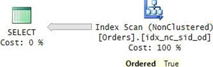
FIGURE 2-62 Execution plan for the query that the cursor is based on.
The important thing to observe in this plan is that the index scan is ordered; therefore, there’s no need for explicit sorting to arrange the data in the order that the query specifies.
The code starts by declaring and opening the cursor. The code declares the cursor as a FAST_FORWARD one, meaning that it’s read-only and forward-only. The code then fetches the first row’s values and puts them into the current row’s variables, and it initially assigns the current row’s variables to the previous row’s variables. Then the code iterates while the last fetch hasn’t reached the end of the cursor (@@fetch_status = 0). In each iteration, the code applies the following:
![]() It checks if the previous shipper ID is different than the current shipper ID. If so, the previous row has the maximum order date for the previous shipper. In such a case, the code checks if that date is before 2010, and if it is, the code returns that shipper ID as a qualifying one.
It checks if the previous shipper ID is different than the current shipper ID. If so, the previous row has the maximum order date for the previous shipper. In such a case, the code checks if that date is before 2010, and if it is, the code returns that shipper ID as a qualifying one.
![]() It assigns the current row’s variables to the previous row’s variables.
It assigns the current row’s variables to the previous row’s variables.
![]() It fetches the next row’s values and puts them into the current row’s variables.
It fetches the next row’s values and puts them into the current row’s variables.
After the loop, the code needs to handle the last row separately to check if the last shipper is a qualifying shipper. Finally, the code closes and deallocates the cursor.
Normally, scanning about 2,500 pages on my system with cold cache takes about half a second. However, because of the high overhead of the iterations and the cursor fetches in T-SQL, it took this solution 17 seconds to complete on my system.
Before you test the set-based solution, run the following code to turn on reporting I/O and time statistics in the session:
SET STATISTICS IO, TIME ON;
You can also enable the Include Actual Execution Plan option in SSMS. It’s OK to do so now because you’re about to run a single statement.
Following is a simple set-based solution for our task (call it set-based solution 1):
SELECT shipperid
FROM dbo.Orders
GROUP BY shipperid
HAVING MAX(orderdate) < '20100101';
The solution uses a basic grouped query against the Orders table. The query groups the rows by shipper ID, and it filters only shipper groups having a maximum order date before 2010. The execution plan for this query is shown in Figure 2-63.
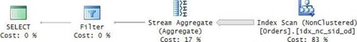
FIGURE 2-63 Query plan for set-based solution 1.
The optimizer created a plan that scans the nonclustered index in order. The plan then applies a stream aggregate based on this order without the need to explicitly sort the rows. Finally, the plan filters the rows that satisfy the HAVING predicate. I got the following performance statistics for this query on my system: logical reads = 2,487, CPU time = 375 ms, elapsed time = 602 ms.
Notice that the run time of this solution is only about half a second. That’s compared with 17 seconds that it took the previous solution to complete. You realize that the plan for this solution uses the same order-based algorithm as in the cursor-based solution. Both solutions scan the same number of pages. The reason that the cursor solution is so much slower is mainly because of the expensive iterations and cursor fetching in T-SQL.
Query tuning with query revisions
Set-based solution 1 is much more efficient than the cursor-based solution. However, what if it’s not efficient enough? Perhaps this is just small-scale test environment with 1,000,000 rows in the Orders table, but suppose the production environment has 100,000,000 rows.
The two operators in the plan in Figure 2-63 that do most of the work are the Index Scan and the Stream Aggregate operators. Both have linear scaling because their cost is proportional to the number of rows involved. Therefore, the whole plan has linear scaling. Simplifying things a bit for the purposes of our discussion, if it takes the query half a second to complete with 1,000,000 rows, it should take it about 50 seconds to complete with 100,000,000 rows. Suppose that you need the query to be much faster than that; say you need it to complete in under three seconds. You did the best you could with rowstore indexes. Now suppose that using columnstore indexing here is not really an option for you. At this point, you should evaluate query revisions that perhaps will result in a more optimal plan.
The idea behind query revisions is that the query optimizer isn’t perfect. Don’t get me wrong; I’m not trying to underestimate its capabilities. But the reality is that, in many cases, different queries that perform the same logical task get different execution plans. This has to do with a number of reasons. The optimizer limits the optimization process so that it won’t become counterproductive. It computes both cost-based and time-based thresholds based on the sizes of the tables involved. If either of the thresholds is reached, the optimization process stops and the optimizer picks the best plan it generated up to that point. With different queries, the starting point for the optimization process is different, so the point where it stops in each case could be after exploring different sets of plans. Also, the use of certain query constructs might impose certain restrictions in terms of the optimizer’s options.
In short, as mentioned, different queries that perform the same logical task can get different plans. Therefore, you have to think of query revisions as a query tuning tool. And if you’d like to improve your query-tuning skills, you should invest time in this area. You should learn how the optimizer tends to handle different query constructs and what changing conditions make the optimizer change its choices. Then, when you tune a query and want to achieve a certain effect on the plan, you will know what to try as opposed to shooting in the dark. I’ll demonstrate this technique on our sample task, and I will show more examples throughout the book.
The first step is to identify the most expensive part in the existing plan. Clearly, that part is the full scan of the leaf level of the nonclustered index.
The second step is to try and identify a more efficient strategy, theoretically, even if you don’t know yet how to achieve it. With a very dense partitioning column (remember, we have a small number of shipper IDs, each with many occurrences in average), the scan strategy isn’t optimal. A far more optimal strategy is to scan the small Shippers table and, per shipper, apply a seek in the nonclustered index on Orders. The seek would reach the right edge of the current shipper’s section in the index leaf and then scan backward one row. That row has the maximum order date for the current shipper. What’s nice about this strategy is that its scaling depends on the number of shippers and not on the number of orders. So, as long as you have a very small number of shippers, that number dictates how many seek operations you will get. Remember that the cost of a seek in an index is as many reads as the number of levels in the index. The number of levels in an index doesn’t change significantly when the number of rows increases. For example, with 1,000,000 rows the index will have three levels, and with 100,000,000 rows it will have four.
The third step is to come up with a query that will get a plan with the desired strategy. You could first try the following query, which returns the maximum order date for a single shipper, just to see if the optimizer will handle it with a seek:
SELECT MAX(orderdate) FROM dbo.Orders WHERE shipperid = 'A';
The plan for this query is shown in Figure 2-64.
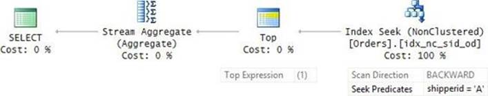
FIGURE 2-64 Query plan for a single shipper.
Sure enough, the plan performs a seek in the nonclustered index to the right edge of shipper A’s section in the index leaf and then starts a backward range scan. The Top operator is the one requesting the rows from the Index Seek operator and, as you can see in the plan, it requests only one row. Therefore, the range scan has no reason to proceed beyond that row. The order date from the filtered row is served to the Stream Aggregate operator, and this operator returns that date as the maximum order date. The execution of this query plan involved three logical reads on my system.
Now that you know that the optimizer applies the desired strategy for a single shipper, the next move is to get the same per shipper from the Shippers table. One way to achieve this is to query the Shippers table and, in the filter, invoke a correlated scalar aggregate subquery that returns the maximum order date for the current shipper. Filter the shipper only if the returned date is before 2010. Here’s the complete solution that implements this approach (call it set-based solution 2):
SELECT shipperid
FROM dbo.Shippers AS S
WHERE (SELECT MAX(orderdate)
FROM dbo.Orders AS O
WHERE O.shipperid = S.shipperid) < '20100101';
One would hope that the plan for this query will start by scanning some index from the Shippers table to get the shipper IDs, and then in a loop perform the activity you saw in Figure 2-64 per shipper. But alas, it is not so, as you can see in the execution plan in Figure 2-65.
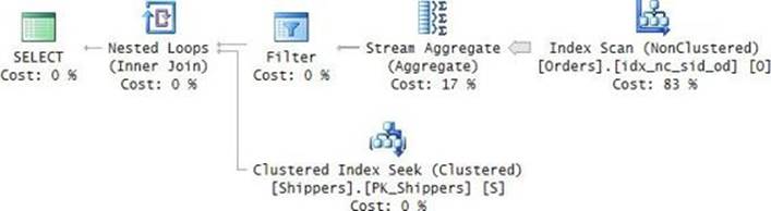
FIGURE 2-65 Query plan for set-based solution 2.
As you can see, the optimizer chose a plan that performs a full scan of the nonclustered index, which is what you were looking to avoid with this query revision. SQL Server reported the following performance statistics for this query on my system: logical reads = 8 + 2487, CPU time = 438 ms, elapsed time = 524 ms.
As it turns out, when the optimizer sees a scalar aggregate subquery like in our example, it first unnests it internally, turning it into a join form. This way, the optimizer can evaluate different plans that access the tables in a different order. The problem is that the optimizer needs to make a number of other decisions here, like which access methods to use to access the tables, which join algorithm to use, which aggregate algorithm to use, and so on. The search space becomes so large that if the optimizer tried to explore all possible plans, the optimization process would become so long that it would be counterproductive. It looks like the optimizer didn’t explore the truly optimal plan here.
Normally, the unnesting of the subqueries that the optimizer performs leads to more efficient plans, but in our case it resulted in an inefficient one. So what you need in this case is to somehow prevent the optimizer from unnesting the subquery, causing it to go to Shippers first and then to Orders per shipper. It would have been handy if SQL Server supported a hint that instructs the optimizer not to unnest the inner query, but unfortunately there’s no such hint. Curiously, there is an indirect way to achieve the same effect. When the subquery uses a TOP filter, SQL Server doesn’t unnest it because, in some cases, such unnesting could change the meaning of the query. The one exception is when the inner query uses TOP (100) PERCENT; in such a case, SQL Server simply ignores the TOP option, knowing that it’s meaningless. So in our query, if you change the subquery to use TOP (1) instead of MAX, it will prevent the undesired unnesting. Here’s the revised solution (call it set-based solution 3):
SELECT shipperid
FROM dbo.Shippers AS S
WHERE (SELECT TOP (1) orderdate
FROM dbo.Orders AS O
WHERE O.shipperid = S.shipperid
ORDER BY orderdate DESC) < '20100101';
The plan for this query is shown in Figure 2-66.
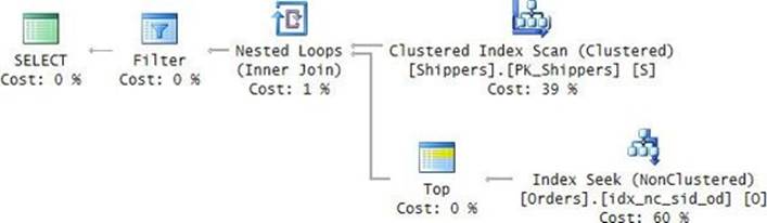
FIGURE 2-66 Query plan for set-based solution 3.
This time, the plan is precisely the desired one. It starts with a scan of the Shippers table, which costs just a couple of reads. This scan returns 12 shipper IDs. Then, per shipper, the loop performs a seek in the nonclustered index on Orders to retrieve the maximum order date for the current shipper. Then the filter keeps the shipper ID if the respective date is before 2010; otherwise, it discards it. Here are the performance statistics I got for this solution: logical reads against Shippers = 2, access count against Orders = 12, logical reads against Orders = 36, CPU time = 0 ms, elapsed time = 12 ms.
Following is another solution that gets an efficient plan (call it set-based solution 4):
SELECT shipperid
FROM dbo.Shippers AS S
WHERE NOT EXISTS
(SELECT * FROM dbo.Orders AS O
WHERE O.shipperid = S.shipperid
AND O.orderdate >= '20100101')
AND EXISTS
(SELECT * FROM dbo.Orders AS O
WHERE O.shipperid = S.shipperid);
You issue the query against the Shippers table. The filter uses a NOT EXISTS predicate with a correlated subquery that ensures that the outer shipper didn’t handle orders placed in 2010 or later. The filter also uses an EXISTS predicate with a correlated subquery that ensures the outer shipper handled at least one order. The plan for this query is shown in Figure 2-67.
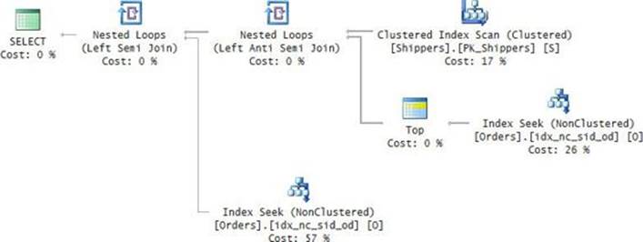
FIGURE 2-67 Query plan for set-based solution 4.
Like the plan for set-based solution 3, this plan also starts with a scan of the Shippers table, which returns 12 shipper IDs. For each of the 12 shippers, the first loop applies a seek in the nonclustered index to check the NOT EXISTS predicate in the query. For each of the remaining shipper IDs (which could be 0 to 12 in our case), the second loop applies a seek in the nonclustered index to check the EXISTS predicate in the query. This plan is a bit more expensive than the one for set-based solution 3, but it’s still highly efficient, and its scaling is also tied to the number of shippers. The performance statistics I got for this query are as follows: logical reads against Shippers = 2, access count against Orders = 19, logical reads against Orders = 72, CPU time = 0 ms, elapsed time = 9 ms.
I covered four different solutions to the task, and each one got a different execution plan. The first was the simplest and most intuitive solution but not the most efficient one. You saw that the remaining attempts to tune the query were not just a matter of trying a bunch of other solutions until you get an efficient one. They were about understanding the inefficiencies in the plan for the first solution and, after thinking about what an efficient plan should look like, applying revisions in an attempt to get certain effects on the plan. The point of this exercise is to emphasize the importance of developing the skill to tune queries based on query revisions.
When you’re done, run the following code to turn off reporting I/O and time statistics in the session:
SET STATISTICS IO, TIME OFF;
At this point, it’s recommended that you rerun the script file PerformanceV3.sql from the book’s source code to re-create the sample database as a clean one.
Parallel query execution
The changes to computer hardware over the past several years have been characterized by huge growth along virtually every possible metric: more and much faster storage, more and faster main memory, and most importantly, more and much more powerful CPUs. A similar set of changes have occurred in databases, with data volumes rapidly growing. Meanwhile, users are ever more demanding of data analytics, but they still expect split-second query times and reports that render at the click of a button.
Processing large volumes of data is naturally easier with a large amount of computing power, but the biggest performance improvements are made by using special algorithms that specifically take advantage of the increased power of newer servers. The key to these algorithms lies in splitting data into smaller chunks that can be distributed across many processor cores at once. Such techniques are referred to as parallel query execution, intraquery parallelism, or simply parallelism, and SQL Server has a mature and nuanced system for handling this kind of work.
This section delves into SQL Server’s parallel query capabilities, focusing on key aspects of query optimization, query execution, and scheduling internals. Understanding these areas will allow you not only to analyze query plans and performance characteristics, but also to control parallelism when necessary, applying it or limiting it as is appropriate for your queries or workload.
![]() Note
Note
The examples in this section use the AdventureWorks2014 sample database. This database is available from CodePlex at https://msftdbprodsamples.codeplex.com/releases/view/125550.
How intraquery parallelism works
Parallel processing—the act of splitting work across multiple processor cores—can be done in several different ways. The most common models are the following:
![]() A factory line model, in which each core takes responsibility for a single action and data is passed from core to core. (Think of an automobile factory, where one person installs door handles, another installs windows, and so on.)
A factory line model, in which each core takes responsibility for a single action and data is passed from core to core. (Think of an automobile factory, where one person installs door handles, another installs windows, and so on.)
![]() A stream-based model, in which each core is responsible for a set of data and performs all the required operations. (This model is similar to a factory in which each car is built completely by a single person.)
A stream-based model, in which each core is responsible for a set of data and performs all the required operations. (This model is similar to a factory in which each car is built completely by a single person.)
Although the factory-line model seems intuitively better, especially when applied to cars and human workers, SQL Server and many other database products are based instead on streaming models. Computer processors, unlike humans, are able to quickly and efficiently switch between tasks, as long as the data is already in the processor’s local cache. Acquiring data from main memory—or, worse, main storage—can be orders of magnitude more expensive than switching to a new task. This means that it is almost always advantageous to do as much work as possible on a given piece of data before moving it along to some other processor or memory location.
Stream-based models also often can scale much better than factory-line models, especially as data sizes grow. SQL Server’s streaming model involves distributing rows across cores as evenly as possible using various algorithms (chosen depending on the scenario). Consider a situation in which a query plan has only three operations but tens of billions of rows on which to apply those operations. In a simple factory-line model, the query plan might be able to use only three processors, but in a streaming model the plan could, in theory, scale to millions or even billions of processor cores. Naturally, there are real-world limits on the number of processor cores that servers ship with, and there is also a point of diminishing returns when massively scaling a data set. But this type of flexibility helps even in smaller cases and is one of the key reasons that a stream-based model is commonly used in database systems.
Basics of parallelism in query plans
The idea of a parallel query plan is a bit of a misnomer. A query plan will be either entirely serial—processed using a single worker thread—or it will include one or more parallel branches, which are areas of the plan that are processed using multiple threads. This is an important distinction, because the query processor has the ability to either merge multiple parallel streams into a single stream or create parallel streams out of a single stream. These operations can be done an arbitrary number of times in a given query plan, meaning that a plan can have numerous parallel zones intermingled with numerous serial zones.
Every parallel zone in a given plan will use the same number of threads as every other parallel zone in the plan. The number of threads per zone is referred to as the degree of parallelism (DOP) for the plan and is determined based on a combination of server settings, plan hints, and run-time server conditions. A given set of threads might be reused by multiple zones over the course of the plan. For example, if your plan has a DOP of 4 and 4 parallel zones, it might use between 4 and 16 actual worker threads to do its work, depending on how the various parallel zones interrelate.
Determining whether or not a given operator is inside of a parallel zone can be done by looking at the icons in the graphical execution plan viewer. Operators that are in parallel zones will be adorned with a circle with two arrows, as shown in Figure 2-68; the Parallelism and Sort operators are in a parallel zone, whereas the Top operator is not.
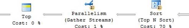
FIGURE 2-68 Operators in parallel zones are decorated with a circle icon with two arrows.
Within a given parallel zone, each worker thread will process a single, unique stream of rows for the entire zone, after which those rows will be moved to another thread in the plan’s next zone (whether that zone is serial or parallel). Therefore, each parallel zone is always bounded on one side by an operator that feeds multiple parallel streams and on the other side by an operator that either redistributes or serializes multiple parallel streams.
Exchange operators
The key feature of parallel query plans is the various parallel zones, and the key to parallel zones is an operator internally referred to as Exchange but exposed in graphical query plans as Parallelism. This operator controls both worker threads and streams of data in parallel plans and, therefore, is the core component that makes parallel plans work.
As a reminder, query plans can be read in two different ways: right to left or left to right. Reading the query plan starting from the right side follows data as it flows through the plan. On the other hand, reading the plan starting from the left side follows the operator logic, which is what actually pulls the data through. Each operator in a plan asks the next downstream operator for one row at a time, and so data streams through the plan.
Most query plan operators are concerned with asking only the next upstream operator for a row and then doing whatever operation or transformation is required before passing the row down the stream. (In the case of blocking operators, like Sort, that might mean acquiring many rows prior to passing one or more back.) Exchange operators deal with multiple streams of rows. However, virtually all other operators on the streams remain blissfully unaware that parallelism is involved.
The Exchange operator has three variants. Each of the three operators has two tasks, which are seemingly in opposition depending on whether you’re reading the plan from a data-flow or operator-logic point of view.
![]() Gather Streams This operator bounds the end of a parallel zone (and the start of a serial zone) when looking at a plan from a data-flow point of view. It takes multiple parallel streams of data and merges them into a single serial stream. When reading a plan from an operator-logic perspective, the Gather Streams operator is actually the start of a parallel zone. Its job from this perspective is to invoke parallel worker threads and ask the operators on each thread for rows.
Gather Streams This operator bounds the end of a parallel zone (and the start of a serial zone) when looking at a plan from a data-flow point of view. It takes multiple parallel streams of data and merges them into a single serial stream. When reading a plan from an operator-logic perspective, the Gather Streams operator is actually the start of a parallel zone. Its job from this perspective is to invoke parallel worker threads and ask the operators on each thread for rows.
![]() Distribute Streams Reading from a data-flow perspective, this operator bounds the start of a parallel zone (likewise, the end of a serial zone). It takes a serial stream of rows and splits it into multiple parallel streams. Reading from an operator-logic perspective, this operator marks the end of a parallel zone; the next upstream operator will be part of a serial zone.
Distribute Streams Reading from a data-flow perspective, this operator bounds the start of a parallel zone (likewise, the end of a serial zone). It takes a serial stream of rows and splits it into multiple parallel streams. Reading from an operator-logic perspective, this operator marks the end of a parallel zone; the next upstream operator will be part of a serial zone.
![]() Repartition Streams The role of this operator is to ingest multiple parallel streams and redistribute the rows onto different threads, based on a different scheme than was used to distribute them in the upstream parallel zone. As such, this operator bounds both the beginning and end of a parallel zone whether the plan is read from a data or logic perspective. Another way to think of this operator is that it joins together two adjacent parallel zones.
Repartition Streams The role of this operator is to ingest multiple parallel streams and redistribute the rows onto different threads, based on a different scheme than was used to distribute them in the upstream parallel zone. As such, this operator bounds both the beginning and end of a parallel zone whether the plan is read from a data or logic perspective. Another way to think of this operator is that it joins together two adjacent parallel zones.
Figure 2-69 shows a query plan that includes all three types of Exchange operators.
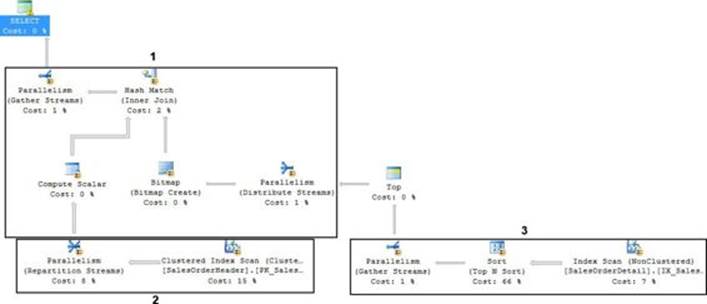
FIGURE 2-69 A query plan that uses all three types of Exchange operators.
The plan shown in Figure 2-69 has been edited and annotated to highlight the three parallel zones (and two serial zones) that are bounded by the various Exchange operators. Parallel zone 1 starts—from a logical perspective—with the Gather Streams operator. The Bitmap operator is fed from a Distribute Streams operator that bounds the zone with a serial zone containing a Top operator. Parallel zone 3 feeds this serial zone and is bounded by a Gather Streams operator. The final parallel zone in the plan—zone 2—is bounded by a Repartition Streams operator and is directly adjacent to zone 1, without an intermediate serial zone.
From a threading point of view, this plan will use a total of DOP * 2 worker threads for its parallel zones, plus a parent thread in the serial zones. The reason that it can use only twice as many worker threads as the DOP, rather than one set of threads per zone, is that the threads allocated for zone 3 will be able to be reused by zone 2.
Again, following the plan’s logical sequence, if DOP is 4, zone 1 will begin and four worker threads will be allocated. The Hash Match operator blocks on its build side—the side that includes parallel zone 3. So this operator will start and will not return until all the work done by the four threads allocated for zone 3 is complete. At this point, the same four threads will be used to process zone 2.
It can be difficult to imagine exactly what is going on when looking at a parallel query plan, but it is somewhat simpler when put into a slightly different graphical form. Consider the plan fragment shown in Figure 2-70.
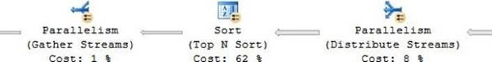
FIGURE 2-70 A parallel zone containing only a Sort operator.
The plan fragment shown in this figure is a complete parallel zone, containing only a Sort operator. If the graphical plan view were rendered in terms of what is really happening, and if the DOP for the plan was 4, the image might instead look similar to what is shown in Figure 2-71.
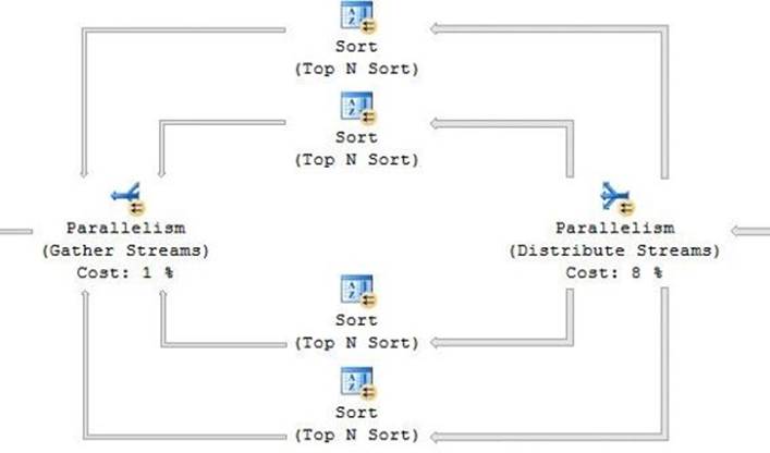
FIGURE 2-71 How parallelism really works.
Given a DOP 4 plan, the Gather Streams operator will allocate four worker threads. Each of these worker threads, in turn, will spawn a Sort operator, and each of these Sort operators will ask the Distribute Streams operator for rows. The important thing to realize is that each of the Sort operators operates entirely independently and completely unaware of what the other Sort operators are doing. Given this design, the DOP can be arbitrarily scaled up or down and the plan can still function the same way, albeit faster or slower.
Inside the Exchange operator
The prior section focused on Exchange operators from a worker-thread and row-stream perspective, but it left a core question unanswered: Why is an Exchange called an Exchange?
Each SQL Server query plan operator has, internally, two logical interfaces: a consumer interface, which takes rows from upstream, and a producer interface, which passes rows downstream. In most operators, these interfaces are handled on the same thread, but in the case of an Exchange, multiple threads will be involved. It is the job of the Exchange operator to take rows from threads on the consumer side and exchange those threads for different threads on the producer side. This is the basis of the name.
The actual exchange process takes place inside of a data structure called CXPacket, where C represents a C++ class (that implements the structure) and XPacket stands for exchange packet, which is the structure’s actual name. As rows are consumed in the operator, they are stored in exchange packets. As the packets fill up with rows, they are passed across the exchange to the thread or threads waiting on the producer side. The number of threads on each side of the exchange depends on the type of exchange: Gather Streams operators will have DOP threads on the consumer side and one thread on the producer side; Distribute Streams operators will have one thread on the consumer side and DOP threads on the producer side; and Repartition Streams operators will have DOP threads on each side of the exchange.
If you have spent some time monitoring SQL Server wait statistics, you no doubt have encountered the CXPACKET wait type. This packet is so named because it involves threads in parallel plans waiting on the CXPacket data structure. Threads with this wait type set are usually waiting for rows on the producer side of the exchange. However, threads on the consumer side can also set the wait type if, for example, some synchronization is necessary prior to the threads beginning to produce rows.
Row-distribution strategies
Parallel query plans must cover a broad set of use cases. To increase the flexibility available to the query optimizer, there are a five options for distributing rows across the threads on the producer side of a Distribute or Repartition exchange:
![]() Hash This is the most common distribution scheme, and it involves each row getting assigned a consumer thread based on the result of a hash function. This scheme is generally used to align rows in logical groups on worker threads. For example, if the hash function is applied to theProductID column, all rows with the same product ID will be assigned to the same worker thread. If the query includes an aggregation grouped by product ID, each thread will be able to independently handle aggregations of several products.
Hash This is the most common distribution scheme, and it involves each row getting assigned a consumer thread based on the result of a hash function. This scheme is generally used to align rows in logical groups on worker threads. For example, if the hash function is applied to theProductID column, all rows with the same product ID will be assigned to the same worker thread. If the query includes an aggregation grouped by product ID, each thread will be able to independently handle aggregations of several products.
![]() Round Robin In this scheme, the first row consumed by the exchange will be distributed to the first thread waiting on the producer side, the second row will be distributed to the second waiting thread, and so on until all threads have received a row. Then the distribution will start again from the first thread. One example of when this scheme is commonly used is on the outside of a Nested Loops operator, where each row represents independent work to be done on the inner side of the loop.
Round Robin In this scheme, the first row consumed by the exchange will be distributed to the first thread waiting on the producer side, the second row will be distributed to the second waiting thread, and so on until all threads have received a row. Then the distribution will start again from the first thread. One example of when this scheme is commonly used is on the outside of a Nested Loops operator, where each row represents independent work to be done on the inner side of the loop.
![]() Broadcast This scheme sends all rows from the consumer side to all threads on the producer side. It is used only when there is a relatively small number of estimated rows and it is desirable for the entire set of rows to be present on each thread—for example, to build a hash table.
Broadcast This scheme sends all rows from the consumer side to all threads on the producer side. It is used only when there is a relatively small number of estimated rows and it is desirable for the entire set of rows to be present on each thread—for example, to build a hash table.
![]() Demand This scheme is unique in that it involves threads on the producer side receiving rows on request. Currently, this is used only in query plans involving aligned partitioned tables.
Demand This scheme is unique in that it involves threads on the producer side receiving rows on request. Currently, this is used only in query plans involving aligned partitioned tables.
![]() Range In this scheme, each thread is given a unique and nonoverlapping range of keys to work with. This scheme is used only when building indexes.
Range In this scheme, each thread is given a unique and nonoverlapping range of keys to work with. This scheme is used only when building indexes.
To see the row distribution scheme and related information used by an Exchange operator, either hover the mouse pointer over the operator until the tooltip appears or, better, click F4 to get a properties window, as shown in Figure 2-72.
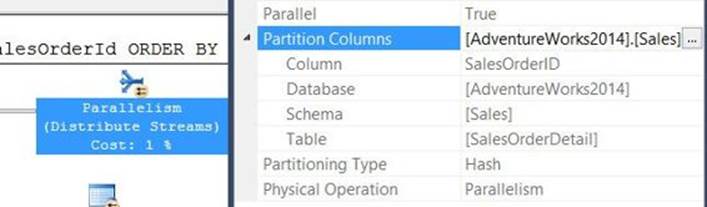
FIGURE 2-72 Getting information about the Exchange operator’s row-distribution scheme.
This figure shows that the selected Distribute Streams operator uses Hash partitioning, and the hash function will be applied to the SalesOrderID column from the AdventureWorks2014 Sales.SalesOrderDetail table.
The properties window has another useful feature for reading parallel query plans: when viewing an actual (as opposed to estimated) query plan, it shows for each operator in the plan—Exchange as well as others—the number of rows that were processed by each worker thread. This information is shown in Figure 2-73.
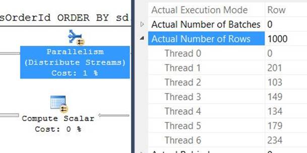
FIGURE 2-73 Viewing the number of rows processed per thread, in an actual query plan.
The number of rows per thread is available by expanding the dialog under the Actual Number Of Rows item. The plan shown here has a DOP of 6, meaning that in each parallel zone there are 6 worker threads. Here each thread processed over 100 rows, but some threads processed more than others; this is probably not a major issue for a plan that deals with only 1,000 rows, but potentially it can cause performance problems for a bigger plan.
Thread 0 here represents the parent thread (also known as the distributor or coordinator thread). This is the thread that is active in serial zones and that spawns the parallel worker threads. Its role here is not to process rows, but rather to control the life cycle of the worker threads; therefore, it does not show as having done any work on this particular operator.
Parallel sort and merging exchange
The main goal of parallelism, of course, is to break expensive units of work into smaller pieces that can run concurrently on more than one CPU. It might be reasonable to expect that if a given operation takes 1,000 ms running on a single processor, it might take only 250 ms running on four processors. This is somewhat naïve logic, but it might be correct—it depends on how expensive it is to split up the work to begin with, and how expensive it is to merge the results back into a single stream so that they can be consumed by the caller.
Surprisingly, there are also cases where splitting up units of work into smaller pieces can actually result in an even greater performance boost than would be expected based on the number of concurrent workers. In other words, for these types of operations, the 1,000-ms example, when run on four processors might take only 200 ms rather than 250 ms. The types of operations for which this works are those that mathematically scale extralinearly; given a working set of size N, these types of operations will perform over 10 times worse for a working set of size N * 10.
One such operation, and by far the most common in database scenarios, is sorting data. The best sort algorithms all scale at the rate of N * LOG(N). This is not a very steep curve: a set of 100,000,000 items will take just over 11 times longer to sort than a set of 10,000,000 items, a difference of only 10 percent compared to a linear scale. However, in the world of database performance, every bit counts. So it makes a lot of sense to take advantage of these kinds of mathematical gains in the query processor.
If a large set of rows needs to be sorted by a given key, the query plan will often put the sort into a parallel zone. If the sort is being done on more than one column, the data will often be distributed using the hash scheme, in order to keep like values together.
Once the data has been sorted, the order often needs to be preserved in a subsequent serial zone; there is little benefit to sorting the data in parallel if it can’t be used. In these cases, the query plan will use a special variant of a Gather Streams operator, known as a merging exchange. A merging exchange consumes multiple streams of data ordered the same way, and it outputs a single stream of data that maintains the same order. This is done using a simple merge algorithm: if the data is sorted by ProductID ascending, rows are read off of each input stream and the minimum ProductID is recorded. Now rows are read off of each stream until there are no more rows for that minimum ID, at which point the next smallest ID is recorded. Rows are now read for that ID, and so on, thereby maintaining the input order.
Figure 2-74 displays a plan fragment for the following query:
SELECT TOP(1000)
UnitPrice
FROM Sales.SalesOrderDetail
ORDER BY
UnitPrice DESC;
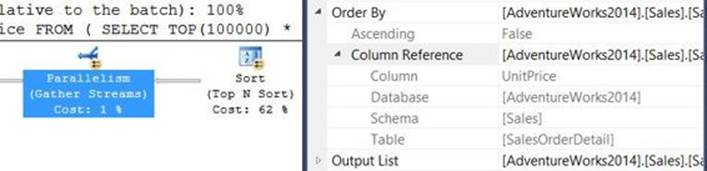
FIGURE 2-74 Parallel sort with merging exchange.
The Gather Streams operator shown here includes an Order By property, indicating that it is a merging exchange. The data will be output ordered by the UnitPrice column from the AdventureWorks2014 Sales.SalesOrderDetail table, which is, in this plan, the same column that the upstream Sort operator uses.
Partial aggregation
When thinking about query plan performance, the most important consideration is generally not how many operators exist in the plan. Most operators process only a single row at a time, and do so very quickly. This is, in fact, the whole point of SQL Server’s streaming query processor model.
The important thing, rather than the number of operators, is how many rows are passing through each operator. Performance problems occur in areas of plans where there are a lot of rows, meaning that the operators are doing a lot of work. It makes sense, therefore, that the earlier in a plan (from a data-flow perspective) that rows can be either filtered or aggregated, the faster that plan will be.
The benefit of early row reduction is more apparent with more expensive operations, and moving data across threads—as is done in Exchange operators—is a very expensive operation. This is because it requires putting the data into exchange packets and then copying those packets to new memory locations, rather than keeping everything in the same place.
To eliminate as much exchange cost as possible, many parallel plans that involve aggregates will use a strategy called partial aggregation. This strategy involves aggregating groups of rows on whatever thread they happen to be on at an earlier point in the plan, and then completing the full aggregation later, after the data has been properly repartitioned.
For example, consider a case where a query is using the MAX aggregate to find the highest price every product in the system has ever sold for. There are 1,000,000 rows for ProductID 123, and these rows are spread across 10 threads. The query processor could repartition all 1,000,000 rows—copying them to new memory locations—and then calculate the aggregate. Or, alternatively, the query processor could calculate one aggregate per thread—the maximum value of all the rows that happen to be on each thread—and then repartition only 10 threads prior to calculating the final aggregate. The answer in either case would be the same, but the cost of repartitioning would be greatly reduced in the latter.
Figure 2-75 shows partial aggregation as the result of the following query:
SELECT
th.ProductID,
th.TransactionDate,
MAX(th.ActualCost) AS MaxCost
FROM
(
SELECT
tha.ProductID,
tha.TransactionDate,
tha.ActualCost
FROM Production.TransactionHistoryArchive AS tha
CROSS JOIN Production.TransactionHistory AS th
) AS th
GROUP BY
th.ProductID,
th.TransactionDate;
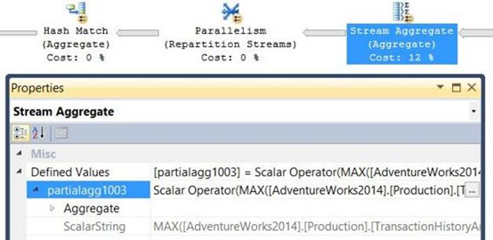
FIGURE 2-75 Partial aggregation.
Here the Stream Aggregate operator calculates a partial aggregate—named within the plan as partialagg1003—which greatly reduces the row count prior to the rows being consumed by the Repartition Streams operator. This plan is chosen because the row estimate is exceptionally large due to the two tables used in the plan being cross joined: An estimated 10,125,100,000 rows will be created by the cross join, but after the initial aggregation only an estimated 319,983 will remain. These rows will be repartitioned, using the Hash scheme, on the combination of the ProductIDand TransactionDate columns. Then the Hash Match operator will finish the aggregation by taking the maximum value of partialagg1003 for each group.
Note that here both Stream Aggregate and Hash Match operators are involved in this partial aggregation, but that is not always the case. Any combination of two aggregate operators can be used to perform partial aggregation.
Parallel scan
Prior to operating on a set of rows, those rows must be read from the heap or index in which they are contained. While this could be accomplished by having a single thread read the data, it is often faster, especially for large tables, to involve several threads in the process. This is done by using a parallel scan.
Figure 2-76 shows a parallel scan as the result of this query:
SELECT
ActualCost
FROM Production.TransactionHistory AS th
ORDER BY
ActualCost DESC;
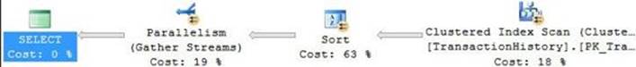
FIGURE 2-76 Parallel scan.
A parallel scan can be a table scan, an index scan, or a range scan—the latter of which will use an operator called Index Seek. There is no special labeling, but a parallel scan is effectively any scan operation done in a parallel zone, except under a nested loop. (That is a special case covered later in this chapter.)
In this plan, the Gather Streams operator spawns worker threads, each of which instantiate a Sort operator. The Sort operators, in turn, ask the Index Scan operator for rows. Because this Index Scan is in a parallel zone, it is parallel aware, and it will not feed the same set of rows to each of the worker threads. Instead, it gives each worker thread a data page or a range of data pages to read, depending on how large the table is. The worker threads read the rows off of the data page or pages, after which they are consumed by the Sort operator. Once all the rows have been read, the worker thread will request more rows from the Scan operator. Scan will once again provide one or more data pages, and it will keep doing so until the entire table or range has been scanned.
The component inside of the Scan operator that takes care of providing the data pages is responsible for figuring out which pages each thread should read next, and also for ensuring that the pages read by each thread are unique so that no two threads will process duplicate rows. The decisions made by this component are largely based upon statistics, so it is even more important than usual to keep statistics up to date when working with large parallel plans.
Few outer rows
One of the key attributes of a high-performance parallel system is that every worker will be equally as busy, and for as long, as every other worker. This means that work has been properly distributed and the work being done in parallel will finish on every worker at about the same time, thereby reducing overall run duration.
Parallel scan works in terms of data pages rather than in terms of rows, and especially with smaller lookup tables there can be cases in which there are fewer data pages than there are worker threads. In such a case, some worker threads would be allocated but would have no work to do, which would mean not only that allocating those threads was a waste of time, but also that the remaining threads would each have to do more work than was expected.
To eliminate this situation, SQL Server implements a special optimization called few outer rows. This optimization occurs when a parallel scan is being used to feed the outer side of a Nested Loops operator. In this case, each row on each thread represents work to be done on the inner side of the loop, and ideally that work should be as evenly distributed among the threads as possible. To accomplish that in a case where the optimizer detects that there will be too few rows, a Repartition Streams operator is injected into the plan immediately following the parallel scan.
Figure 2-77 shows the result of this optimization on behalf of the following query:
SELECT
p.ProductId,
th0.TransactionID
FROM Production.Product AS p
CROSS APPLY
(
SELECT TOP(1000)
th.TransactionId
FROM Production.TransactionHistory AS th
WHERE
th.ProductID = p.ProductID
ORDER BY
th.TransactionID
) AS th0
ORDER BY
th0.TransactionId;
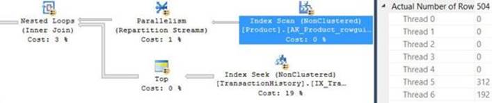
FIGURE 2-77 Without the few outer rows optimization, only two of six threads would have work to do.
In this plan, the index scan of the Product table results in only two of the six worker threads receiving rows. This is because there are only two data pages in the index; the table has only 504 rows. The query optimizer has foreseen this issue and included a Repartition Streams operator directly after the scan. This operator will repartition the rows using the Round Robin scheme, thereby producing perfect balance across the workers, as shown in Figure 2-78.
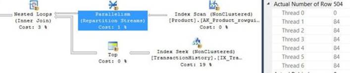
FIGURE 2-78 The Round Robin scheme equally distributes rows among the worker threads.
Parallel hash join and bitmap
It is extremely common—given that parallel query plans tend to work with large sets of rows and that hash match is designed to join large sets of rows—to see Hash Join operators in parallel query plans. Therefore, it makes sense that these joins should be as optimized as possible.
The usual hash join algorithm involves hashing the outer (build-side) keys, hashing each inner (probe-side) key, finding the matching bucket in the hash table, and finally walking the bucket’s linked list to find the matching row.
In parallel plans, an optimization can occur whereby each thread will build a bitmap with the same number of bits as the number of buckets in the hash table. A bit in the bitmask will be 0 if there are no rows in the corresponding hash bucket and 1 if there are rows in the hash bucket. At probe time, rather than going straight into the hash bucket, the query processor can instead first discover, by means of the bitmap, whether or not there might be a potential row in the hash table. This can greatly reduce the cost and overhead of hash join queries, especially in cases where a large proportion of probe-side rows do not match a build-side row.
The following query is optimized with a bitmap in the plan, as shown in Figure 2-79:
SELECT
*
FROM
(
SELECT
sh.*,
sd.ProductId
FROM
(
SELECT TOP(1000)
*
FROM Sales.SalesOrderDetail
ORDER BY
SalesOrderDetailId
) AS sd
INNER JOIN Sales.SalesOrderHeader AS sh ON
sh.SalesOrderId = sd.SalesOrderId
) AS s;
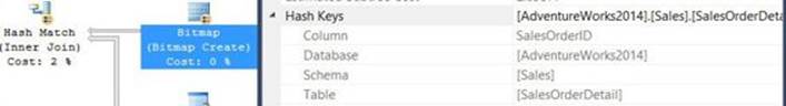
FIGURE 2-79 A hash bitmap in a parallel plan.
The bitmap in these kinds of plans, as shown here, is based on the same hash keys as the subsequent Hash Match operator.
A further enhancement of the bitmap optimization can occur in data-warehouse queries that the query optimizer has determined to be part of a star join (one or more dimensions joining to a fact table). If the star join optimization occurs, each of the dimensions will be scanned and internally merged into a single bitmap (and hash table) that can be used on the probe side as a single filter. This approach can be significantly faster than separately probing a hash table for each dimension.
Parallelism and partitioned tables
In parallel plans involving tables with a large number of partitions, the query optimizer might choose to distribute threads and individually process each partition, rather than sequentially scanning the entire set of partitions using the typical parallel scan mechanism. This special case involves the Demand distribution scheme; each thread can work on a single partition at a time and request another partition to work on once the first one is done. In this way, the work is well balanced across worker threads, even when some partitions have fewer rows than others.
Seeing this in action requires a partitioned table, so some setup is needed. The following code creates a partition function, a partition scheme, and a table in tempdb:
USE tempdb;
GO
CREATE PARTITION FUNCTION pf_1 (INT)
AS RANGE LEFT FOR VALUES
(
25000, 50000, 75000, 100000,
125000, 150000, 175000, 200000,
225000, 250000, 275000, 300000,
325000, 350000, 375000, 400000,
425000, 450000, 475000, 500000,
525000, 550000, 575000, 600000,
625000, 650000, 675000, 700000,
725000, 750000, 775000, 800000,
825000, 850000, 875000, 900000,
925000, 950000, 975000, 1000000
);
GO
CREATE PARTITION SCHEME ps_1
AS PARTITION pf_1 ALL TO ([PRIMARY]);
GO
CREATE TABLE dbo.partitioned_table
(
col1 INT NOT NULL,
col2 INT NOT NULL,
some_stuff CHAR(200) NOT NULL DEFAULT('')
) ON ps_1(col1);
GO
CREATE UNIQUE CLUSTERED INDEX ix_col1
ON dbo.partitioned_table
(
col1
) ON ps_1(col1);
GO
The partition function specifies 41 partitions (including the implicit partition for values greater than 1,000,000), and the table is clustered based on col1 used in conjunction with the partition scheme. The table includes two integer columns and a CHAR(200) column that is used to increase the query cost in order to influence the optimization process. (See the discussion later in this chapter for more detail.)
Once the table has been created, some data can be inserted:
WITH
n1 AS (SELECT 1 a UNION ALL SELECT 1),
n2 AS (SELECT 1 a FROM n1 b, n1 c),
n3 AS (SELECT 1 a FROM n2 b, n2 c),
n4 AS (SELECT 1 a FROM n3 b, n3 c),
n5 AS (SELECT 1 a FROM n4 b, n4 c),
n6 AS (SELECT 1 a FROM n5 b, n5 c)
INSERT INTO dbo.partitioned_table WITH (TABLOCK)
(
col1,
col2
)
SELECT TOP(1000000)
ROW_NUMBER() OVER
(
ORDER BY
(SELECT NULL)
) AS col1,
CHECKSUM(NEWID()) AS col2
FROM n6;
GO
This query generates and inserts 1,000,000 rows into the table. The col1 column will contain sequential values between 1 and 1,000,000, whereas the values in col2 will be pseudorandom, based on a checksum of a unique identifier.
Once the table has been populated with data, the following query can be used, which produces the plan fragment shown in Figure 2-80:
SELECT
COUNT(*)
FROM partitioned_table AS pt1
INNER JOIN partitioned_table AS pt2 ON
pt1.col1 = pt2.col1
WHERE
pt1.col1 BETWEEN 25000 AND 500000;
GO
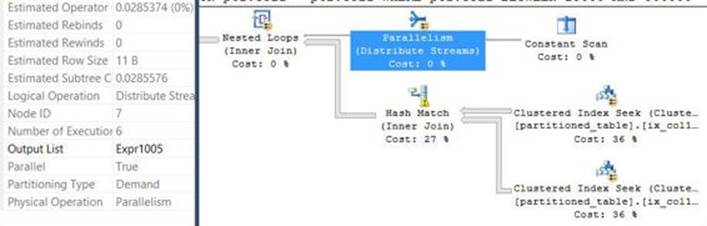
FIGURE 2-80 Demand-based row distribution in a plan involving partitioned tables.
The Constant Scan used in this plan returns one row per partition that will need to be accessed, as determined by the query optimizer based on the predicate in the WHERE clause of the query. The Distribute Streams operator consumes these rows and then distributes them based on the Demand scheme, as shown on the Properties tab to the left of the plan fragment.
Parallel SELECT INTO
For several years, it has been possible to do parallel bulk loads of data into tables by using the Bulk Copy API. A parallel bulk load does not involve query-processor parallelism, but rather enables client applications to spawn multiple concurrent bulk loads that can run together. This works because a minimally logged bulk copy deals only with page allocations; several streams allocating pages simultaneously has no risk of conflict nor requirement for concurrency except in the page allocation structures, so this is a low overhead and simple way to improve throughput.
Within the query engine itself, T-SQL developers have long been able to do minimally logged inserts by using the SELECT INTO syntax (as long as the target database uses either the Simple or Bulk Logged recovery model). However, these operations have always written data using a single stream even though the relational engine is capable of handling multiple concurrent streams.
Consider the following SELECT INTO query:
WITH
n1 AS (SELECT 1 a UNION ALL SELECT 1),
n2 AS (SELECT 1 a FROM n1 b, n1 c),
n3 AS (SELECT 1 a FROM n2 b, n2 c),
n4 AS (SELECT 1 a FROM n3 b, n3 c),
n5 AS (SELECT 1 a FROM n4 b, n4 c),
n6 AS (SELECT 1 a FROM n5 b, n5 c)
SELECT TOP(10000000)
ROW_NUMBER() OVER
(
ORDER BY
(SELECT NULL)
) AS col1,
CHECKSUM(NEWID()) AS col2
INTO #test_table
FROM n6;
This query inserts 10,000,000 rows into a temporary table called #test_table. Figure 2-81 shows a fragment of the query plan when this query is run against a SQL Server 2012 instance.
![]()
FIGURE 2-81 In SQL Server 2012, SELECT INTO writes on a single thread.
Even though this query uses parallelism, prior to calculating the row number, the parallel streams are gathered. After the row number is calculated, the data is written to the temp table on a single serial stream.
The same query, run against a SQL Server 2014 instance, generates the plan fragment shown in Figure 2-82.
![]()
FIGURE 2-82 In SQL Server 2014, SELECT INTO can do multithreaded writes.
In SQL Server 2014, the row number is still generated in a serial zone. However, once it has been calculated, the rows are distributed to multiple threads (in this case, using the Round Robin scheme) and are then written to the destination temporary table from multiple simultaneous streams.
The performance benefit of this enhancement can be surprisingly large: on one test server that has both SQL Server 2012 and SQL Server 2014 installed, with identical disk systems and memory allocations, the query runs for 10 seconds in SQL Server 2012 and only for 4 seconds in SQL Server 2014.
Parallelism and query optimization
Prior to the query processor being able to exercise a parallel query plan, the query optimizer must generate one. The process that is used is somewhat more complex and nuanced than that used for serial query plans, and as a developer working with parallel queries you need to understand what is going on in order to effectively deal with problems as they occur.
The decision to use or not use parallelism in a query plan is mostly made prior to the query processor’s role in plan execution. This decision is based on a combination of instance-level (or Resource Governor workload group-level) settings and the query in question. The execution engine that actually runs the plan has very little say in whether or not parallelism is used, and it will veto its use only when the SQL Server instance is under extreme resource pressure.
Parallelism settings
A discussion of the parallel query optimization process is impossible without an understanding of the instance-level and Resource Governor settings that influence the process.
There are four instance-level settings that can influence parallelism. These settings can be viewed in the sys.configurations catalog view and can be configured using the sp_configure system stored procedure. The settings are as follows:
![]() Affinity Mask This setting controls which of the server’s logical processors will be mapped to a SQLOS scheduler. A parallel query plan requires more than one SQLOS scheduler, so if the affinity mask is set such that there is only a single mapped processor, the query optimizer will not attempt to produce parallel query plans. That said, it is quite rare to see a single-scheduler SQL Server instance given the commonality of multicore processors in today’s servers. The default value for this setting is 0, which indicates that all logical processors should be mapped to SQLOS schedulers.
Affinity Mask This setting controls which of the server’s logical processors will be mapped to a SQLOS scheduler. A parallel query plan requires more than one SQLOS scheduler, so if the affinity mask is set such that there is only a single mapped processor, the query optimizer will not attempt to produce parallel query plans. That said, it is quite rare to see a single-scheduler SQL Server instance given the commonality of multicore processors in today’s servers. The default value for this setting is 0, which indicates that all logical processors should be mapped to SQLOS schedulers.
![]() Max Degree of Parallelism The maximum degree of parallelism is a default value that is used by parallel queries to determine how many worker threads to allocate per parallel zone (the DOP previously discussed). This setting can be overridden—either increased or decreased—using the query-level MAXDOP hint. The maximum in this setting’s name and the query hint are both a bit misleading; if a query uses parallelism, it will use whatever DOP is specified at the query level, by this setting, or by the Resource Governor setting described later in this section. There is neither a query optimizer decision nor a run-time query processor decision made about what the “correct” DOP might be for a given query. The default for this setting is 0, which means that each zone of a parallel plan can use as many threads as there are online SQLOS schedulers, up to 64.
Max Degree of Parallelism The maximum degree of parallelism is a default value that is used by parallel queries to determine how many worker threads to allocate per parallel zone (the DOP previously discussed). This setting can be overridden—either increased or decreased—using the query-level MAXDOP hint. The maximum in this setting’s name and the query hint are both a bit misleading; if a query uses parallelism, it will use whatever DOP is specified at the query level, by this setting, or by the Resource Governor setting described later in this section. There is neither a query optimizer decision nor a run-time query processor decision made about what the “correct” DOP might be for a given query. The default for this setting is 0, which means that each zone of a parallel plan can use as many threads as there are online SQLOS schedulers, up to 64.
![]() Cost Threshold for Parallelism When optimizing query plans, the query optimizer goes through multiple stages, each of which adds time and expense to the process. One of the central goals of the optimizer is to produce a good enough plan in a short amount of time, and this setting helps it achieve that goal by allowing it to exit the query-optimization process if a serial version of a query’s plan does not have a high enough cost to warrant further optimization. The default for this setting is 5, which means that only serial plans with a cost higher than 5 will be put through the parallel-optimization phases.
Cost Threshold for Parallelism When optimizing query plans, the query optimizer goes through multiple stages, each of which adds time and expense to the process. One of the central goals of the optimizer is to produce a good enough plan in a short amount of time, and this setting helps it achieve that goal by allowing it to exit the query-optimization process if a serial version of a query’s plan does not have a high enough cost to warrant further optimization. The default for this setting is 5, which means that only serial plans with a cost higher than 5 will be put through the parallel-optimization phases.
![]() Max Worker Threads SQLOS maintains an internal pool of operating system threads that are used (and reused) by queries as needed. Threads are finite resources and must be carefully controlled to avoid process starvation issues, so a given SQL Server instance is limited in how many threads it can create at any given time. This setting controls that limit, and this is the only setting that can have a run-time impact, rather than an optimization-time impact. If the query processor determines that the server is close to running out of worker threads, it will downgrade a parallel query plan to a serial query plan (by using a DOP of 1) in an attempt to keep the server from hitting the wall. The default for this setting is 0, which means that the instance controls the number of threads based on the number of logical processors. This system is fully documented at the following URL: http://msdn.microsoft.com/en-us/library/ms190219.aspx.
Max Worker Threads SQLOS maintains an internal pool of operating system threads that are used (and reused) by queries as needed. Threads are finite resources and must be carefully controlled to avoid process starvation issues, so a given SQL Server instance is limited in how many threads it can create at any given time. This setting controls that limit, and this is the only setting that can have a run-time impact, rather than an optimization-time impact. If the query processor determines that the server is close to running out of worker threads, it will downgrade a parallel query plan to a serial query plan (by using a DOP of 1) in an attempt to keep the server from hitting the wall. The default for this setting is 0, which means that the instance controls the number of threads based on the number of logical processors. This system is fully documented at the following URL: http://msdn.microsoft.com/en-us/library/ms190219.aspx.
In addition to these instance-level settings, a given Resource Governor workload group can override the Max Degree Of Parallelism setting by using the Resource Governor max_dop setting. This setting has the same implications as the instance-level setting, except that it interacts differently with the query-level MAXDOP hint: the Resource Governor setting can be overridden by the query level hint, but it can be only lessened, and not increased. In other words, if max_dop is set to 10 by Resource Governor, a T-SQL developer can override it in a given query to 8, but not to 12. This is a useful way to control complex ad hoc workloads and ensure that a single query does not consume too many resources.
The optimization process
In the first phase of query optimization, the optimizer produces a serial version of a query plan for the query. The query plan has a total cost, which is the sum of the cost determined for each operator in the plan. These costs are further broken down, on each operator, into CPU and I/O costs, as shown in Figure 2-83.
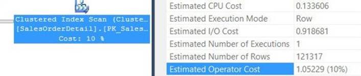
FIGURE 2-83 The operator costs for an index scan in a serial plan.
In the plan fragment shown, this serial scan has an estimated CPU cost of 0.133606, an estimated I/O cost of 0.918681, and a total operator cost of 1.05229—the sum of the CPU and I/O costs.
Once the serial plan has been generated, the costs for each of the operators in the plan are added together. If the total is less than the value of the Cost Threshold For Parallelism setting, no further optimization is attempted and the plan is used as-is. If, however, the total exceeds the Cost Threshold For Parallelism, the query is subjected to further optimization phases, and parallel query plans are considered.
Once a parallel query plan has been generated for a query, additional math takes place. Each operator’s CPU cost—but not its I/O cost—is divided by the number referred to as the DOP for costing. This number is the lesser of half of the number of SQLOS schedulers, or the MAXDOP that will be used by the plan as a result of settings or the MAXDOP query hint. For example, on an instance with 24 schedulers, the DOP for costing will be 12 if the Max Degree Of Parallelism setting is left untouched and the query is left unhinted. If the query-level MAXDOP hint is set to 8, that number will be used instead. However, on an instance with 12 schedulers, the DOP for costing will be 6 even if the MAXDOP hint is set to 8, because the lesser of the two values is used.
Figure 2-84 shows the same index scan as the prior figure, this time in a parallel plan.
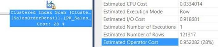
FIGURE 2-84 The CPU cost has been divided by the DOP for costing.
In this case, the query was optimized on an instance with 8 SQLOS schedulers, but with the instance-level Max Degree Of Parallelism set to 6. The serial CPU cost of 0.133606 has been divided by 4—half of the number of schedulers—to yield an estimated parallel CPU cost of 0.0334014. The I/O cost remains untouched, because SQL Server takes a conservative approach in assuming that the I/O channel will be fully saturated. The result, even without touching the I/O cost, is a lower overall operator cost.
The new operator costs are all added together, in addition to the operator costs for any Exchange operators that were added to the plan to facilitate parallel processing. If the total operator cost of the parallel version of the plan is less than the total operator cost of the serial version of the plan, the query optimizer chooses the parallel version. Otherwise, the serial version is used.
Configuring an instance for parallelism
No discussion of settings would be complete without some advice for configuration. Unfortunately, there are no simple answers, but some general guidelines can be helpful.
The Affinity Mask and Max Worker Threads settings, in the vast majority of cases, should be left untouched.
Affinity Mask was primarily intended to control licensing agreements, but recent versions of SQL Server must be licensed for all the processors available on a given server. This leaves edge cases where, for example, SQL Server shares a server with an IIS instance and the administrator wants to give each process its own reserved CPUs. This use case does make some sense, but in today’s world, server virtualization technologies are usually a better way to handle that situation.
The Max Worker Threads setting is designed to be automatically maintained and should generally need adjustment only in extreme cases with especially heavy parallel workloads and specific symptoms indicative of thread-pool exhaustion. These cases will generally necessitate a call to product support, and it is probably wise to allow the support person to decide how best to fix the situation.
Query cost is a metric that was first introduced in SQL Server 7.0, back in 1998. Now, 16 years later, as of the time of this writing, the computer industry has changed dramatically, but query costs still use the same basic structure. A query with a cost of 5, the default for Cost Threshold Of Parallelism, was quite large in 1998, but in today’s massive databases it is relatively small. It is therefore recommended that this number be changed for most SQL Server instances. A value between 30 and 50 makes sense given today’s typical hardware and data sizes. You might consider setting things even higher if you are seeing small queries (for your environment) using parallel plans.
Like Cost Threshold For Parallelism, the Max Degree Of Parallelism setting has an unfortunate default. This setting should be tuned for a given instance in an effort to balance the goals of fast query response time and allowing many queries to run concurrently. If Max Degree Of Parallelism is set too low, large queries will slow down; if it is set too high, concurrent queries will be forced to compete for processor time and therefore will interact negatively.
General guidelines for Max Degree Of Parallelism depend on the workload. For OLTP systems, which tend to have a much higher percentage of small serial query plans in addition to much lighter-weight larger queries, a smaller Max Degree Of Parallelism—as low as 2—might be advised.
For OLAP workloads, on the other hand, a smaller number of much larger queries is typical and a higher Max Degree Of Parallelism is usually a good idea. It is wise to start, on a four-socket server, with the number of processors per NUMA node (usually the same as the number of processors per socket), or half that number on a two-socket server. This gives each query a significant portion of the available CPU power, while allowing several concurrent queries to run without interacting.
If Hyper-Threading is enabled, it is recommended that you set Max Degree Of Parallelism to no more than 50 percent higher than the number of physical processors per node. In other words, if there are 6 physical processors per node and 12 logical processors (due to Hyper-Threading), it is generally advisable to set Max Degree Of Parallelism no higher than 9. This helps to keep query execution from overwhelming the additional boost provided by Hyper-Threading.
Parallelism inhibitors
In addition to the core query optimization and processing decisions, several query features can inhibit parallelism in one of two ways: either forcing a serial zone in an otherwise parallel query plan, or disabling parallelism entirely for a given query.
Following is a list of the common things that will cause a serial region to appear in a parallel query plan:
![]() Multistatement T-SQL UDF A multistatement UDF returns a tabular value via a table variable. The logic in the user-defined function (UDF) will be processed in a serial zone, although the rest of the plan might use parallelism.
Multistatement T-SQL UDF A multistatement UDF returns a tabular value via a table variable. The logic in the user-defined function (UDF) will be processed in a serial zone, although the rest of the plan might use parallelism.
![]() Recursive CTEs Recursive common table expressions are processed in serial zones, although downstream operators might still use parallelism.
Recursive CTEs Recursive common table expressions are processed in serial zones, although downstream operators might still use parallelism.
![]() Backward scans Indexes in SQL Server use doubly linked lists that can be scanned in either a forward or backward direction. Only forward scans are eligible for the parallel scan already described. Backward scans will be done in serial.
Backward scans Indexes in SQL Server use doubly linked lists that can be scanned in either a forward or backward direction. Only forward scans are eligible for the parallel scan already described. Backward scans will be done in serial.
![]() Nonpartitioned TOP, aggregates, and windowing functions Use of the TOP operator, aggregations, and windowing functions all involve creating groups of rows. If the group must be determined by analyzing the entire set of input rows at a given stage of the plan, the query optimizer has no choice but to use a serial zone. Examples include TOP outside of a correlated table expression, an ungrouped aggregate (also known as a scalar aggregate), and a windowing function that doesn’t use partitioning.
Nonpartitioned TOP, aggregates, and windowing functions Use of the TOP operator, aggregations, and windowing functions all involve creating groups of rows. If the group must be determined by analyzing the entire set of input rows at a given stage of the plan, the query optimizer has no choice but to use a serial zone. Examples include TOP outside of a correlated table expression, an ungrouped aggregate (also known as a scalar aggregate), and a windowing function that doesn’t use partitioning.
The following list includes common features that will completely disable parallelism for a given plan:
![]() Scalar T-SQL UDF Use of any scalar T-SQL UDF in a query will make that query unable to use parallelism. This should be a major red flag for any developer thinking of using T-SQL UDFs. Inline expressions or CLR scalar UDFs are often better options.
Scalar T-SQL UDF Use of any scalar T-SQL UDF in a query will make that query unable to use parallelism. This should be a major red flag for any developer thinking of using T-SQL UDFs. Inline expressions or CLR scalar UDFs are often better options.
![]() Modification of table variables In most cases, when inserting, updating, or deleting rows in a table using a query, the parts of the query prior to the actual data modification can be processed in a parallel zone. (The data modification will always be processed in a serial zone, with the exception of parallel SELECT INTO.) Table variables break this precedent; if rows in a table variable are being modified, the entire plan will run serially. Note that this is not the case if the table variable is merely used in some part of the plan not involving row modification.
Modification of table variables In most cases, when inserting, updating, or deleting rows in a table using a query, the parts of the query prior to the actual data modification can be processed in a parallel zone. (The data modification will always be processed in a serial zone, with the exception of parallel SELECT INTO.) Table variables break this precedent; if rows in a table variable are being modified, the entire plan will run serially. Note that this is not the case if the table variable is merely used in some part of the plan not involving row modification.
![]() CLR UDFs with DataAccessKind.Read CLR UDFs will not disable parallelism unless the UDF is marked with DataAccessKind.Read, which means that it has access to run a query in the hosting database.
CLR UDFs with DataAccessKind.Read CLR UDFs will not disable parallelism unless the UDF is marked with DataAccessKind.Read, which means that it has access to run a query in the hosting database.
![]() Memory-optimized tables Memory-optimized tables cannot participate in parallel query plans.
Memory-optimized tables Memory-optimized tables cannot participate in parallel query plans.
To see the impact of one of these features, first consider the following query, the plan for which is shown in Figure 2-85:
SELECT TOP(1000)
OrderQty
FROM Sales.SalesOrderDetail
ORDER BY
OrderQty DESC;
GO

FIGURE 2-85 A parallel query plan.
This query generates a typical parallel plan; but what if a small modification is made? First create the following scalar UDF:
CREATE FUNCTION dbo.ReturnInput(@input INT)
RETURNS INT
AS
BEGIN
RETURN(@input)
END
GO
Once the UDF is created, it can be used in the query:
SELECT TOP(1000)
dbo.ReturnInput(OrderQty)
FROM Sales.SalesOrderDetail
ORDER BY
OrderQty DESC;
GO
Despite the fact that it is probably the simplest UDF that can possibly be written, its impact on the query plan is extreme, as shown in Figure 2-86.

FIGURE 2-86 No longer a parallel query plan.
If you are trying to figure out whether your plan is not parallel as a result of the presence of an inhibitor, check the properties of the SELECT operator. Figure 2-87 highlights the NonParallelPlanReason property, which can help you understand what might be keeping parallelism at bay.
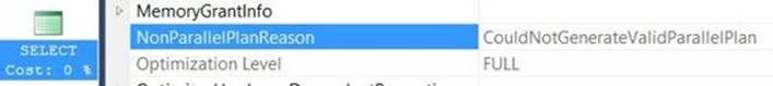
FIGURE 2-87 The NonParallelPlanReason node shows that an inhibitor is present.
In this case, the NonParallelPlanReason node shows that it is impossible to generate a valid parallel plan—in other words, the inhibitor is invalidating things. Looking at this property for a plan that you expect to be parallel tells you to look for and remove inhibitors.
The parallel APPLY query pattern
Given the extra-linear properties of scale described earlier in the chapter, in addition to the overhead associated with migrating rows between threads, large parallel query plans often don’t scale as well as might be ideal.
Although the query optimizer is capable of performing a number of optimizations and transformations on any given query, its scope is somewhat limited based on its model. By using more extensive manual rewrites, you often can create plans that perform up to an order of magnitude faster, without hoping that the query optimizer will arrive at the right solution.
An example query
The AdventureWorks2014 sample database, although handy for example queries, is not quite big enough to illustrate the benefits or drawbacks of various performance techniques. To write a sample query, a few larger tables are required.
First, let’s look at a table with five times more products than the standard version:
SELECT
p.Name,
p.ProductID + x.v AS ProductID
INTO #bigger_products
FROM Production.Product AS p
CROSS JOIN
(
VALUES
(0),(1000),(2000),(3000),(4000)
) AS x(v);
CREATE CLUSTERED INDEX i_ProductID
ON #bigger_products (ProductID);
GO
The #bigger_products table is created by cross-joining the 504 rows from Production.Product with five new rows, and then adding a number to each row to create a total of 2,520 rows. This table is clustered on ProductID.
Next, here’s a table with 504 times more transactions than the standard version:
SELECT
th.ProductID + x.v AS ProductID,
th.ActualCost,
th.TransactionDate
INTO #bigger_transactions
FROM Production.TransactionHistory AS th
CROSS JOIN
(
SELECT
(NTILE(5) OVER (ORDER BY p.ProductId) - 1) * 1000
FROM Production.Product AS p
) AS x(v);
CREATE CLUSTERED INDEX i_ProductID
ON #bigger_transactions (ProductID);
GO
This table is created by cross-joining the 113,443 transactions in Production.TransactionHistory with 504 rows derived from Production.Product. The NTILE function is used to create five groups of rows that correspond to the five rows used to create the #bigger_products table. The resultant set has 57,175,272 rows and is also clustered on the ProductID column. This was chosen because the example query will use this column to join the two tables.
The scenario is as follows: a user would like to know, for each product, the top 10 highest prices (including ties) for which that product was sold, as well as the dates of the transactions. The following query answers the question:
SELECT
p.Name,
x.TransactionDate,
x.ActualCost
FROM
(
SELECT
th.ProductID,
th.TransactionDate,
th.ActualCost,
ROW_NUMBER() OVER
(
PARTITION BY
th.ProductId
ORDER BY
th.ActualCost DESC
) AS rn
FROM #bigger_transactions AS th
) AS x
INNER JOIN #bigger_products AS p ON
p.ProductID = x.ProductID
WHERE
x.rn <= 10;
This query works by calculating a row number in derived table x, partitioned by ProductID and ordered by ActualCost descending. On the outer side of the query, the rows are filtered to return only the top 10 per product, and a join is made to #bigger_products to obtain each product’s name. Figure 2-88 shows a version of the plan that has been edited to fit in this book.
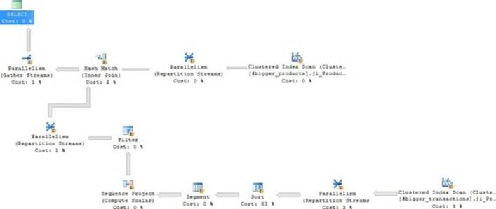
FIGURE 2-88 The query plan for finding the top 10 most expensive transactions.
This query plan uses parallelism, but it has a couple of potential bottlenecks that can be solved without modifying either indexes or table structure.
The first bottleneck is the sort on the probe side of the Hash Join operator. As already mentioned, Sort does not scale linearly, and in this case the number of input rows is quite large. The set will be split up because this is a parallel plan, but the reduction in size will be limited by the DOP of the plan. Splitting the set into even smaller working subsets could potentially yield a larger benefit. Furthermore, smaller subsets require less memory and have less of a chance of running out of memory and spilling to tempdb.
The second bottleneck is the Repartition Streams used just downstream from the parallel scan on the probe side of the Hash Join operator. This operator uses the Hash distribution methodology to distribute rows among the threads based on ProductID. This is done so that the rows for each product will be properly sorted together. Unfortunately, because this repartition is necessary so early in the plan, it must move every row produced by the scan—all 57,175,272 of them. That is a lot of data movement.
Parallel nested loops
The solution to both of these bottlenecks is to rethink the way data flows through a big plan like this one and work out a way to eliminate monolithic operations and instead do many more, but much smaller, operations. The query plan tool that can make this happen is the Nested Loops operator.
In any query plan, whether it is serial or parallel, a Nested Loops operator invokes its inner-side operators once per outer row. Nested Loops is often used with correlated subqueries or table expressions as a way to evaluate the correlated expression for every necessary row.
From the perspective of join performance, Nested Loops is generally not the best choice for large sets of data, because each inner-side evaluation requires another seek or scan of the data and the cost of these operations can add up. For this reason, Hash or Merge joins are usually used as data volumes increase.
That said, in many queries join performance is not the main thing that determines overall performance. Because of the scalability curve of both the Sort and Repartition Streams operator, the join performance in the plan shown in Figure 2-88 is greatly overshadowed by other elements. In this and similar examples, you are better off ignoring join performance and focusing on the bigger picture. Leveraging Nested Loops will allow you to properly handle this situation.
Reducing parallel plan overhead
The key to leveraging Nested Loops is a special query technique known as the Parallel APPLY Pattern. This pattern is shown in Listing 2-1.
LISTING 2-1 The Parallel APPLY Pattern
SELECT
p.[columns]
FROM [driver_table] AS x
[CROSS | OUTER] APPLY
(
SELECT
[columns]
FROM [correlated_table] AS c
WHERE
c.[key] = x.[key]
) AS p
The pattern has two primary elements:
![]() Driver table This is a table (or set of rows) where each row represents a unique piece of work to be done in the inner table expression. For example, this table might be a set of products, customers, dates, or some similar element type over which you would like to do an analysis on a per-item basis.
Driver table This is a table (or set of rows) where each row represents a unique piece of work to be done in the inner table expression. For example, this table might be a set of products, customers, dates, or some similar element type over which you would like to do an analysis on a per-item basis.
![]() Correlated table (or tables) The rows in the driver table should be able to correlate to rows in the table expression via a key. Ideally, correlation should be nonoverlapping, such that each row in the outer driver table represents a specific and unique set in the inner expression. Ideally, the inner table or tables should use covering indexes so that key lookups will be unnecessary.
Correlated table (or tables) The rows in the driver table should be able to correlate to rows in the table expression via a key. Ideally, correlation should be nonoverlapping, such that each row in the outer driver table represents a specific and unique set in the inner expression. Ideally, the inner table or tables should use covering indexes so that key lookups will be unnecessary.
Applying this pattern to the example query is simply a matter of rewriting the inner join using a CROSS APPLY, as follows:
SELECT
p.Name,
x.TransactionDate,
x.ActualCost
FROM #bigger_products AS p
CROSS APPLY
(
SELECT
th.TransactionDate,
th.ActualCost,
ROW_NUMBER() OVER
(
ORDER BY
th.ActualCost DESC
) AS rn
FROM #bigger_transactions AS th
WHERE
th.ProductID = p.ProductID
) AS x
WHERE
x.rn <= 10;
This version of the query starts with the #bigger_products table; because the join is done on ProductID and the row number is calculated by partitioning on ProductID, each product represents a unique piece of work in the query plan. By driving a loop off of rows from #bigger_products, the query will exercise the inner table expression once per product. The inner table expression is correlated on ProductID, so the explicit PARTITION BY clause is removed from the ROW_NUMBER function.
The resultant query has exactly the same logic as the prior version, but the query plan changes significantly, as shown in Figure 2-89.
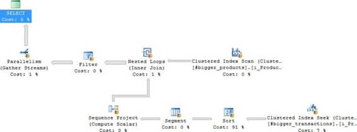
FIGURE 2-89 Parallel APPLY query plan for finding the top 10 most expensive transactions.
This query plan now includes one inner-side index operation per product. That is undoubtedly more expensive than the single parallel scan used in the previous version of the query. But that increased cost is much more than made up for by much smaller sorts and the lack of needing an inner-side repartition.
Running these queries side by side on a test server with Max Degree Of Parallelism set to 6 gives conclusive results: the initial version of the query runs for 31 seconds, and the rewritten version completes in 15. Bigger or more complex queries will see even greater performance improvements when this pattern is properly leveraged.
Conclusion
This chapter covered various query and index tuning topics. It introduced you to internal data structures, fundamental index access methods, tools to measure query performance, and other tuning aspects. So much is involved in tuning, and knowledge of the product’s architecture and internals plays a big role in doing it well. But knowledge is not enough. I hope this chapter gave you the tools and guidance for putting your knowledge into action as you progress in this book—and, of course, in your production environments.
All materials on the site are licensed Creative Commons Attribution-Sharealike 3.0 Unported CC BY-SA 3.0 & GNU Free Documentation License (GFDL)
If you are the copyright holder of any material contained on our site and intend to remove it, please contact our site administrator for approval.
© 2016-2026 All site design rights belong to S.Y.A.