T-SQL Querying (2015)

Chapter 11. Graphs and recursive queries

This chapter covers the treatment of specialized data structures called graphs in Microsoft SQL Server using T-SQL. People use different terms when they want to discuss a graph, like hierarchy and tree, but those terms are often used incorrectly. For this reason, the chapter starts with a terminology section describing graphs and their properties to clear up the confusion.

The treatment of graphs in a relational database management system (RDBMS) is far from trivial. I’ll discuss the two main approaches. One is based on iterative or recursive logic—for example, using recursive queries. Another is based on materializing extra information in the database that describes the data structure—for example, using the HIERARCHYID data type.

Terminology

This chapter uses many terms to discuss graphs and how to manipulate them in SQL Server. This section provides definitions of important terms to make sure you understand them.

Note

The explanations in this section are based on definitions from the National Institute of Standards and Technology (NIST). I made some revisions and added some narrative to the original definitions to make them less formal and keep them relevant to the subject area (T-SQL).

For more complete and formal definitions of graphs and related terms, refer to http://www.nist.gov/dads/.

Graphs

A graph is a set of items connected by edges. Each item is called a vertex or node. An edge is a connection between two nodes of a graph.

Graph is a catchall term for a data structure, and many scenarios can be represented as graphs—for example, employee organizational charts, bills of materials (BOMs), road systems, and so on. To narrow down the type of graph to a more specific case, you need to identify its properties:

Directed/Undirected In a directed graph (also known as a digraph), the two nodes of an edge have a direction or order—as if one is the major node and the other is the minor node. For example, in a BOM graph for coffee shop products, you might have nodes named Latte and Milk. Latte contains Milk, but you cannot turn that relationship around. The graph has an edge (a containment relationship) for the pair of nodes (Latte, Milk), but it has no edge for the pair (Milk, Latte).

In an undirected graph, each edge simply connects two nodes, with no particular order. For example, a road-system graph could have a road between Los Angeles and San Francisco. The edge (road) between the nodes (cities) Los Angeles and San Francisco can be expressed as either of the following: {Los Angeles, San Francisco} or {San Francisco, Los Angeles}.

Acyclic/Cyclic An acyclic graph is a graph with no cycle—that is, no path that starts and ends at the same node. Examples include employee organizational charts and BOMs. A directed acyclic graph is also known as a DAG.

If the graph has paths that start and end at the same node—as there usually are in road systems—the graph is not acyclic. In other words, the graph is cyclic.

Trees

A tree is a data structure accessed beginning at the root node. Each node is either a leaf node or an internal node. An internal node has one or more child nodes and is called the parent of its child nodes. All child nodes of the same node are siblings. A tree is an acyclic graph. Contrary to the appearance in a physical tree, the root is usually depicted at the top of the structure and the leaves are depicted at the bottom, as illustrated in Figure 11-1.

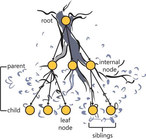
FIGURE 11-1 Roles of nodes in a tree.

A forest is a collection of one or more trees—for example, forum discussions can be represented as a forest in which each thread is a tree.

Hierarchies

Some scenarios can be described as hierarchies and modeled as directed acyclic graphs—for example, inheritance among types and classes in object-oriented programming and reports-to relationships in an employee organizational chart. In the former scenario, the edges of the graph locate the inheritance. Classes can inherit methods and properties from other classes (and possibly from multiple classes). In the latter scenario, the edges represent the reports-to relationship between employees. Note the directed, acyclic nature of these scenarios. The management chain of responsibility in a company cannot go around in circles, for example.

Scenarios

Throughout the chapter, I will use three scenarios: Employee Organizational Chart (tree, hierarchy); Bill of Materials, or BOM (DAG); and Road System (undirected cyclic graph). Note what distinguishes a (directed) rooted tree from a DAG. All trees are DAGs, but not all DAGs are trees. In a tree, an item can have at most one parent.

Employee organizational chart

The employee organizational chart I will use is depicted graphically in Figure 11-2.

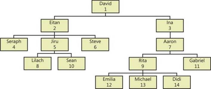
FIGURE 11-2 Employee organizational chart.

To create the Employees table and populate it with sample data, run the code in Listing 11-1. The contents of the Employees table are shown in Table 11-1.

LISTING 11-1 Data-definition language and sample data for the Employees table

SET NOCOUNT ON;
USE tempdb;
IF OBJECT_ID(N'dbo.Employees', 'U') IS NOT NULL DROP TABLE dbo.Employees;
GO
CREATE TABLE dbo.Employees
(
empid INT NOT NULL CONSTRAINT PK_Employees PRIMARY KEY,
mgrid INT NULL CONSTRAINT FK_Employees_Employees REFERENCES dbo.Employees,
empname VARCHAR(25) NOT NULL,
salary MONEY NOT NULL,
CHECK (empid <> mgrid)
);

INSERT INTO dbo.Employees(empid, mgrid, empname, salary) VALUES
(1, NULL, 'David' , $10000.00),
(2, 1, 'Eitan' , $7000.00),
(3, 1, 'Ina' , $7500.00),
(4, 2, 'Seraph' , $5000.00),
(5, 2, 'Jiru' , $5500.00),
(6, 2, 'Steve' , $4500.00),
(7, 3, 'Aaron' , $5000.00),
(8, 5, 'Lilach' , $3500.00),
(9, 7, 'Rita' , $3000.00),
(10, 5, 'Sean' , $3000.00),
(11, 7, 'Gabriel', $3000.00),
(12, 9, 'Emilia' , $2000.00),
(13, 9, 'Michael', $2000.00),
(14, 9, 'Didi' , $1500.00);

CREATE UNIQUE INDEX idx_unc_mgrid_empid ON dbo.Employees(mgrid, empid);

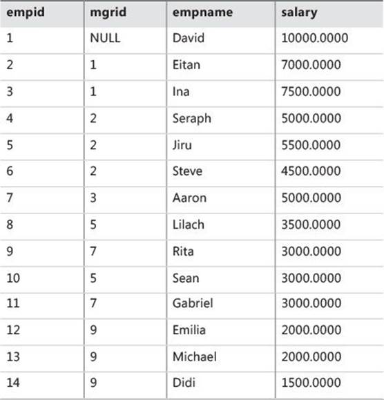
TABLE 11-1 Contents of Employees table

The Employees table represents a management hierarchy as an adjacency list, where the manager and employee represent the parent and child nodes, respectively.

Bill of materials (BOM)

I will use a BOM of coffee shop products, which is depicted graphically in Figure 11-3.

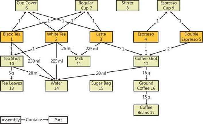
FIGURE 11-3 Bill of materials (BOM) for coffee shop products.

To create the Parts and BOM tables and populate them with sample data, run the code in Listing 11-2. The contents of the Parts and BOM tables are shown in Tables 11-2 and 11-3.

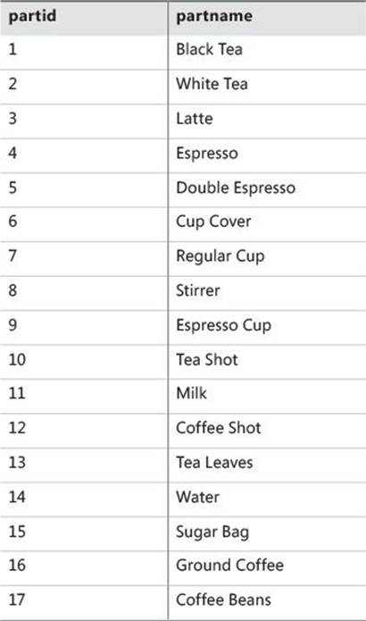
TABLE 11-2 Contents of Parts table

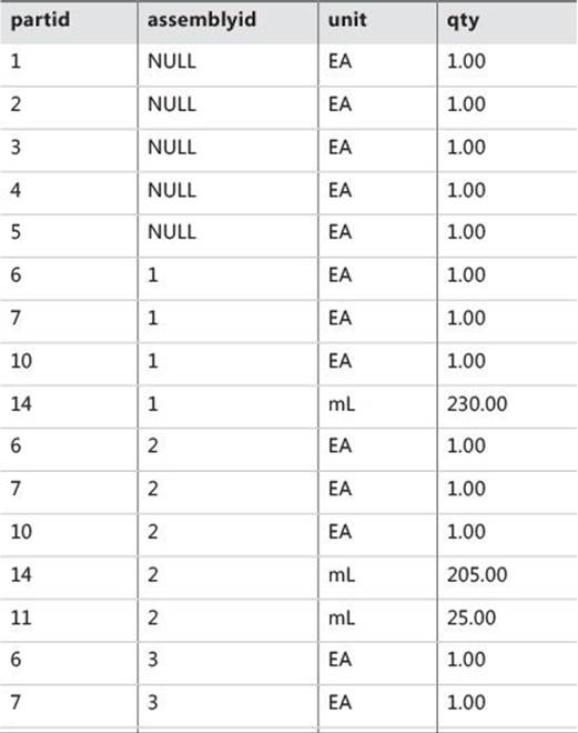
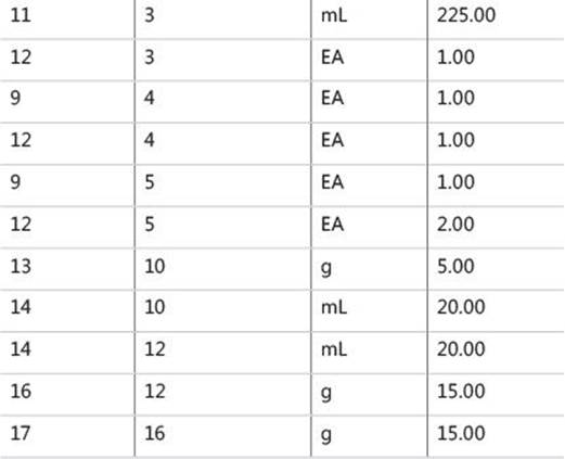
TABLE 11-3 Contents of BOM table

Notice that the first scenario (employee organizational chart) requires only one table because it is modeled as a tree; both an edge (manager, employee) and a node (employee) can be represented by the same row. The BOM scenario requires two tables because it is modeled as a DAG, where multiple paths can lead to each node. An edge (assembly, part) is represented by a row in the BOM table, and a node (part) is represented by a row in the Parts table.

LISTING 11-2 Data-definition language and sample data for the Parts and BOM tables

IF OBJECT_ID(N'dbo.BOM', N'U') IS NOT NULL DROP TABLE dbo.BOM;
IF OBJECT_ID(N'dbo.Parts', N'U') IS NOT NULL DROP TABLE dbo.Parts;
GO
CREATE TABLE dbo.Parts
(
partid INT NOT NULL CONSTRAINT PK_Parts PRIMARY KEY,
partname VARCHAR(25) NOT NULL
);

INSERT INTO dbo.Parts(partid, partname) VALUES
( 1, 'Black Tea' ),
( 2, 'White Tea' ),
( 3, 'Latte' ),
( 4, 'Espresso' ),
( 5, 'Double Espresso'),
( 6, 'Cup Cover' ),
( 7, 'Regular Cup' ),
( 8, 'Stirrer' ),
( 9, 'Espresso Cup' ),
(10, 'Tea Shot' ),
(11, 'Milk' ),
(12, 'Coffee Shot' ),
(13, 'Tea Leaves' ),
(14, 'Water' ),
(15, 'Sugar Bag' ),
(16, 'Ground Coffee' ),
(17, 'Coffee Beans' );

CREATE TABLE dbo.BOM
(
partid INT NOT NULL CONSTRAINT FK_BOM_Parts_pid REFERENCES dbo.Parts,
assemblyid INT NULL CONSTRAINT FK_BOM_Parts_aid REFERENCES dbo.Parts,
unit VARCHAR(3) NOT NULL,
qty DECIMAL(8, 2) NOT NULL,
CONSTRAINT UNQ_BOM_pid_aid UNIQUE(partid, assemblyid),
CONSTRAINT CHK_BOM_diffids CHECK (partid <> assemblyid)
);

INSERT INTO dbo.BOM(partid, assemblyid, unit, qty) VALUES
( 1, NULL, 'EA', 1.00),
( 2, NULL, 'EA', 1.00),
( 3, NULL, 'EA', 1.00),
( 4, NULL, 'EA', 1.00),
( 5, NULL, 'EA', 1.00),
( 6, 1, 'EA', 1.00),
( 7, 1, 'EA', 1.00),
(10, 1, 'EA', 1.00),
(14, 1, 'mL', 230.00),
( 6, 2, 'EA', 1.00),
( 7, 2, 'EA', 1.00),
(10, 2, 'EA', 1.00),
(14, 2, 'mL', 205.00),
(11, 2, 'mL', 25.00),
( 6, 3, 'EA', 1.00),
( 7, 3, 'EA', 1.00),
(11, 3, 'mL', 225.00),
(12, 3, 'EA', 1.00),
( 9, 4, 'EA', 1.00),
(12, 4, 'EA', 1.00),
( 9, 5, 'EA', 1.00),
(12, 5, 'EA', 2.00),
(13, 10, 'g' , 5.00),
(14, 10, 'mL', 20.00),
(14, 12, 'mL', 20.00),
(16, 12, 'g' , 15.00),
(17, 16, 'g' , 15.00);

The BOM represents a directed acyclic graph (DAG). It holds the parent and child node IDs in the assemblyid and partid attributes, respectively. The BOM also represents a weighted graph, where a weight or number is associated with each edge. In our case, that weight is the qty attribute that holds the quantity of the part within the assembly (the assembly of subparts). The unit attribute holds the unit of the qty (EA for each, g for gram, mL for milliliter, and so on).

Road system

The Road System scenario I will use refers to road systems for several major cities in the United States, and it is depicted graphically in Figure 11-4. In this scenario, I chose an International Air Transport Association (IATA) code to identify each city.

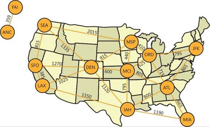
FIGURE 11-4 Road-system scenario.

To create the Cities and Roads tables and populate them with sample data, run the code in Listing 11-3. The contents of the Cities and Roads tables are shown in Tables 11-4 and 11-5.

LISTING 11-3 Data-definition language and sample data for the Cities and Roads tables

IF OBJECT_ID(N'dbo.Roads', N'U') IS NOT NULL DROP TABLE dbo.Roads;
IF OBJECT_ID(N'dbo.Cities', N'U') IS NOT NULL DROP TABLE dbo.Cities;
GO
CREATE TABLE dbo.Cities
(
cityid CHAR(3) NOT NULL CONSTRAINT PK_Cities PRIMARY KEY,
city VARCHAR(30) NOT NULL,
region VARCHAR(30) NULL,
country VARCHAR(30) NOT NULL
);

INSERT INTO dbo.Cities(cityid, city, region, country) VALUES
('ATL', 'Atlanta', 'GA', 'USA'),
('ORD', 'Chicago', 'IL', 'USA'),
('DEN', 'Denver', 'CO', 'USA'),
('IAH', 'Houston', 'TX', 'USA'),
('MCI', 'Kansas City', 'KS', 'USA'),
('LAX', 'Los Angeles', 'CA', 'USA'),
('MIA', 'Miami', 'FL', 'USA'),
('MSP', 'Minneapolis', 'MN', 'USA'),
('JFK', 'New York', 'NY', 'USA'),
('SEA', 'Seattle', 'WA', 'USA'),
('SFO', 'San Francisco', 'CA', 'USA'),
('ANC', 'Anchorage', 'AK', 'USA'),
('FAI', 'Fairbanks', 'AK', 'USA');

CREATE TABLE dbo.Roads
(
city1 CHAR(3) NOT NULL CONSTRAINT FK_Roads_Cities_city1 REFERENCES dbo.Cities,
city2 CHAR(3) NOT NULL CONSTRAINT FK_Roads_Cities_city2 REFERENCES dbo.Cities,
distance INT NOT NULL,
CONSTRAINT PK_Roads PRIMARY KEY(city1, city2),
CONSTRAINT CHK_Roads_citydiff CHECK(city1 < city2),
CONSTRAINT CHK_Roads_posdist CHECK(distance > 0)
);

INSERT INTO dbo.Roads(city1, city2, distance) VALUES
('ANC', 'FAI', 359),
('ATL', 'ORD', 715),
('ATL', 'IAH', 800),
('ATL', 'MCI', 805),
('ATL', 'MIA', 665),
('ATL', 'JFK', 865),
('DEN', 'IAH', 1120),
('DEN', 'MCI', 600),
('DEN', 'LAX', 1025),
('DEN', 'MSP', 915),
('DEN', 'SEA', 1335),
('DEN', 'SFO', 1270),
('IAH', 'MCI', 795),
('IAH', 'LAX', 1550),
('IAH', 'MIA', 1190),
('JFK', 'ORD', 795),
('LAX', 'SFO', 385),
('MCI', 'ORD', 525),
('MCI', 'MSP', 440),
('MSP', 'ORD', 410),
('MSP', 'SEA', 2015),
('SEA', 'SFO', 815);

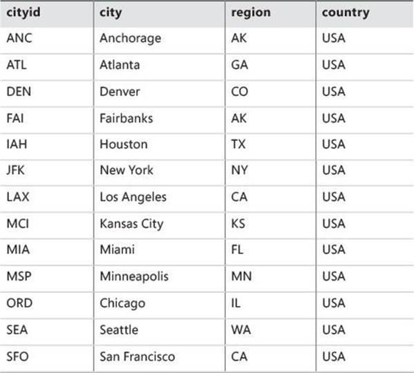
TABLE 11-4 Contents of Cities table

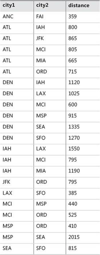
TABLE 11-5 Contents of Roads table

The Roads table represents an undirected cyclic weighted graph. Each edge (road) is represented by a row in the table. The attributes city1 and city2 are two city IDs representing the nodes of the edge. The weight in this case is the distance attribute, which holds the distance between the cities in miles. Note that the Roads table has a CHECK constraint (city1 < city2) as part of its schema definition to reject attempts to enter the same edge twice (for example, {SEA, SFO} and {SFO, SEA}).

Having all the scenarios and sample data in place, let’s go over the approaches to the treatment of graphs. I’ll cover three main approaches: iterative/recursive, materialized path, and nested sets.

Iteration/recursion

Iterative approaches apply some form of loops or recursion. Many iterative algorithms traverse graphs. Some traverse graphs a node at a time and are usually implemented with cursors, but these are typically very slow. I will focus on algorithms that traverse graphs one level at a time using a combination of iterative or recursive logic and set-based queries. Given a set of nodes P, the next level refers to the set C, which consists of the children of the nodes in P. In my experience, implementations of iterative algorithms that traverse a graph one level at a time perform much better than the ones that traverse a graph one node at a time.

Using iterative solutions has several advantages over the other methods. First, you don’t need to materialize any extra information describing the graph to the database other than the node IDs in the edges. In other words, you don’t need to redesign your tables. The solutions traverse the graph by relying solely on the stored edge information—for example, (mgrid, empid), (assemblyid, partid), (city1, city2), and so on.

Second, most of the solutions that apply to trees also apply to the more generic digraphs. In other words, most solutions that apply to graphs where only one path can lead to a given node also apply to graphs where multiple paths may lead to a given node.

Finally, most of the solutions I will describe in this section support a virtually unlimited number of levels.

There are two ways to implement iterative solutions: with loops or with recursive common table expressions (CTEs). The core algorithms are similar in both cases. The use of loops can result in better performance because you have more control over the physical side of things. You can work with your own temporary tables, define your own indexing on them, and so on. Especially when you know what you’re doing, you can achieve good performance. As for recursive CTEs, on the downside they give you very little control over the physical side of things. SQL Server does spool interim sets in internal work tables, but it gives you no control over their structure and indexing. On the upside, recursive CTEs are less verbose and more elegant.

If you want to encapsulate the logic of your loop-based solutions, you can use either multistatement, table-valued user-defined functions (UDFs) or stored procedures. From the user perspective, UDFs are more convenient to work with because you query them like you query tables. However, stored procedures are much less restricted, and you can typically achieve better performance with them. For example, in stored procedures you can materialize and index interim sets in temporary tables, which have histograms. Multistatement, table-valued UDFs use table variables, which have no histograms. So, with temporary tables the query optimizer tends to produce better estimates, which in turn tend to lead to more efficient query plans. That said, I chose to use UDFs in my examples for the loop-based solutions because I want to focus on the algorithms and the clarity of the code. You can easily convert those to stored procedures with temporary tables if you like.

As for the solutions that use recursive CTEs, if you want to encapsulate their logic in a routine, you can use an inline (rather than a multistatement) table-valued UDF. There’s no performance downside to this option because, from an optimization perspective, the use of inline UDFs is transparent. The code gets inlined by definition. In the examples of recursive CTEs in this chapter, I use ad hoc code with local variables in the following form:

DECLARE @input AS <data_type>;

<recursive_query>;

To encapsulate the logic in an inline UDF, simply use the following form:

CREATE FUNCTION <function_name>(@input AS <data_type>) RETURNS TABLE
AS
RETURN
<recursive_query>;

Subgraph/descendants

Let’s start with a classical request to return a subgraph (also known as descendants) of a given root in a digraph; for example, return all subordinates of a given employee. When the graph qualifies as a tree, the request is usually referred to as a subtree. The iterative algorithm is simple:

Input: @root

Algorithm:

• set @lvl = 0; insert into table @Subs row for @root

• while there were rows in the previous level of employees:

• set @lvl += 1; insert into table @Subs rows for the next level (mgrid in (empid values in previous level))

• return @Subs

Run the following code to create the Subordinates1 UDF, which implements this algorithm.

---------------------------------------------------------------------
-- Function: Subordinates1, Descendants
--
-- Input : @root INT: Manager id
--
-- Output : @Subs Table: id and level of subordinates of
-- input manager (empid = @root) in all levels
--
-- Process : * Insert into @Subs row of input manager
-- * In a loop, while previous insert loaded more than 0 rows
-- insert into @Subs next level of subordinates
---------------------------------------------------------------------
IF OBJECT_ID(N'dbo.Subordinates1', N'TF') IS NOT NULL DROP FUNCTION dbo.Subordinates1;
GO
CREATE FUNCTION dbo.Subordinates1(@root AS INT) RETURNS @Subs TABLE
(
empid INT NOT NULL PRIMARY KEY NONCLUSTERED,
lvl INT NOT NULL,
UNIQUE CLUSTERED(lvl, empid) -- Index will be used to filter level
)
AS
BEGIN
DECLARE @lvl AS INT = 0; -- Initialize level counter with 0

-- Insert root node into @Subs
INSERT INTO @Subs(empid, lvl)
SELECT empid, @lvl FROM dbo.Employees WHERE empid = @root;

WHILE @@rowcount > 0 -- while previous level had rows
BEGIN
SET @lvl += 1; -- Increment level counter

-- Insert next level of subordinates to @Subs
INSERT INTO @Subs(empid, lvl)
SELECT C.empid, @lvl
FROM @Subs AS P -- P = Parent
INNER JOIN dbo.Employees AS C -- C = Child
ON P.lvl = @lvl - 1 -- Filter parents from previous level
AND C.mgrid = P.empid;
END

RETURN;
END
GO

The function accepts the @root input parameter, which is the ID of the requested subtree’s root employee. The function returns the @Subs table variable, with all subordinates of employee with ID = @root in all levels. Besides containing the employee attributes, @Subs also has a column called lvl that keeps track of the level in the subtree (0 for the subtree’s root and increasing from there by 1 in each iteration).

The function’s code keeps track of the current level being handled in the @lvl local variable, which is initialized with zero.

The function’s code first inserts into @Subs the row from Employees where empid = @root.

Then in a loop, while the last insert affects more than zero rows, the code increments the @lvl variable’s value by one and inserts into @Subs the next level of employees—in other words, direct subordinates of the managers inserted in the previous level.

To insert the next level of employees into @Subs, the query in the loop joins @Subs (representing managers) with Employees (representing subordinates).

The lvl column is important because you can use it to isolate the managers that were inserted into @Subs in the last iteration. To return only subordinates of the previously inserted managers, the join condition filters from @Subs only rows where the lvl column is equal to the previous level (@lvl – 1).

To test the function, run the following code, which returns the subordinates of employee 3:

SELECT empid, lvl FROM dbo.Subordinates1(3) AS S;

This code generates the following output:

empid lvl
----------- -----------
3 0
7 1
9 2
11 2
12 3
13 3
14 3

You can verify that the output is correct by examining Figure 11-2 and following the subtree of the input root employee (ID = 3).

To get other attributes of the employees in addition to just the employee ID, you can either rewrite the function and add those attributes to the @Subs table or simply join the function with the Employees table, like so:

SELECT E.empid, E.empname, S.lvl
FROM dbo.Subordinates1(3) AS S
INNER JOIN dbo.Employees AS E
ON E.empid = S.empid;

You get the following output:

empid empname lvl
----------- ------------------------- -----------
3 Ina 0
7 Aaron 1
9 Rita 2
11 Gabriel 2
12 Emilia 3
13 Michael 3
14 Didi 3

To limit the result set to leaf employees under the given root, simply add a filter with a NOT EXISTS predicate to select only employees that are not managers of other employees:

SELECT empid
FROM dbo.Subordinates1(3) AS P
WHERE NOT EXISTS
(SELECT * FROM dbo.Employees AS C
WHERE c.mgrid = P.empid);

This query returns employee IDs 11, 12, 13, and 14.

So far, you’ve seen a UDF implementation of a subtree under a given root, which contains a WHILE loop. The following code has the CTE solution, which contains no explicit loop:

DECLARE @root AS INT = 3;

WITH Subs AS
(
-- Anchor member returns root node
SELECT empid, empname, 0 AS lvl
FROM dbo.Employees
WHERE empid = @root

UNION ALL

-- Recursive member returns next level of children
SELECT C.empid, C.empname, P.lvl + 1
FROM Subs AS P
INNER JOIN dbo.Employees AS C
ON C.mgrid = P.empid
)
SELECT empid, empname, lvl FROM Subs;

This code generates the following output:

empid empname lvl
----------- ------------------------- -----------
3 Ina 0
7 Aaron 1
9 Rita 2
11 Gabriel 2
12 Emilia 3
13 Michael 3
14 Didi 3

The solution applies logic similar to the UDF implementation. It’s simpler in the sense that you don’t need to explicitly define the returned table or filter the previous level’s managers.

The first query in the CTE’s body returns the row from Employees for the given root employee. It also returns zero as the level of the root employee. In a recursive CTE, a query that doesn’t have any recursive references is known as an anchor member.

The second query in the CTE’s body (following the UNION ALL operator) has a recursive reference to the CTE’s name. This makes it a recursive member, and it is treated in a special manner. The recursive reference to the CTE’s name (Subs) represents the result set returned previously. The recursive member query joins the previous result set, which represents the managers in the previous level, with the Employees table to return the next level of employees. The recursive query also calculates the level value as the employee’s manager level plus one. The first time that the recursive member is invoked, Subs stands for the result set returned by the anchor member (root employee). There’s no explicit termination check for the recursive member; rather, it is invoked repeatedly until it returns an empty set. Thus, the first time it is invoked, it returns direct subordinates of the subtree’s root employee. The second time it is invoked, Subs represents the result set of the first invocation of the recursive member (first level of subordinates), so it returns the second level of subordinates. The recursive member is invoked repeatedly until there are no more subordinates—in which case, it returns an empty set and recursion stops.

The reference to the CTE name in the outer query represents the unified result sets returned by the invocation of the anchor member and all the invocations of the recursive member.

As I mentioned earlier, using iterative logic to return a subgraph of a digraph where multiple paths might exist to a node is similar to returning a subtree. Run the following code to create the PartsExplosion function:

---------------------------------------------------------------------
-- Function: PartsExplosion, Parts Explosion
--
-- Input : @root INT: assembly id
--
-- Output : @PartsExplosion Table:
-- id and level of contained parts of input part
-- in all levels
--
-- Process : * Insert into @PartsExplosion row of input root part
-- * In a loop, while previous insert loaded more than 0 rows
-- insert into @PartsExplosion next level of parts
---------------------------------------------------------------------
IF OBJECT_ID(N'dbo.PartsExplosion', N'TF') IS NOT NULL DROP FUNCTION dbo.PartsExplosion;
GO
CREATE FUNCTION dbo.PartsExplosion(@root AS INT) RETURNS @PartsExplosion Table
(
partid INT NOT NULL,
qty DECIMAL(8, 2) NOT NULL,
unit VARCHAR(3) NOT NULL,
lvl INT NOT NULL,
n INT NOT NULL IDENTITY, -- surrogate key
UNIQUE CLUSTERED(lvl, n) -- Index will be used to filter lvl
)
AS
BEGIN
DECLARE @lvl AS INT = 0; -- Initialize level counter with 0

-- Insert root node to @PartsExplosion
INSERT INTO @PartsExplosion(partid, qty, unit, lvl)
SELECT partid, qty, unit, @lvl
FROM dbo.BOM
WHERE partid = @root;

WHILE @@rowcount > 0 -- while previous level had rows
BEGIN
SET @lvl = @lvl + 1; -- Increment level counter

-- Insert next level of subordinates to @PartsExplosion
INSERT INTO @PartsExplosion(partid, qty, unit, lvl)
SELECT C.partid, P.qty * C.qty, C.unit, @lvl
FROM @PartsExplosion AS P -- P = Parent
INNER JOIN dbo.BOM AS C -- C = Child
ON P.lvl = @lvl - 1 -- Filter parents from previous level
AND C.assemblyid = P.partid;
END

RETURN;
END
GO

The function accepts a part ID representing an assembly in a BOM, and it returns the parts explosion (the direct and indirect subitems) of the assembly. The implementation of the PartsExplosion function is similar to the implementation of the function Subordinates1. The row for the root part is inserted into the @PartsExplosion table variable (the function’s output parameter). And then in a loop, while the previous insert returned rows, the next level parts are inserted into @PartsExplosion. A small addition here is specific to a BOM: calculating the quantity. The root part’s quantity is simply the one stored in the part’s row. The contained (child) part’s quantity is the quantity of its containing (parent) item multiplied by its own quantity.

Run the following code to test the function, which returns the part explosion of partid 2 (White Tea):

SELECT P.partid, P.partname, PE.qty, PE.unit, PE.lvl
FROM dbo.PartsExplosion(2) AS PE
INNER JOIN dbo.Parts AS P
ON P.partid = PE.partid;

This code generates the following output:

partid partname qty unit lvl
------- ------------ ------- ---- ----
2 White Tea 1.00 EA 0
6 Cup Cover 1.00 EA 1
7 Regular Cup 1.00 EA 1
10 Tea Shot 1.00 EA 1
14 Water 205.00 mL 1
11 Milk 25.00 mL 1
13 Tea Leaves 5.00 g 2
14 Water 20.00 mL 2

You can check the correctness of this output by examining Figure 11-3.

Following is the CTE solution for the parts explosion, which, again, is similar to the subtree solution with the addition of the quantity calculation:

DECLARE @root AS INT = 2;

WITH PartsExplosion
AS
(
-- Anchor member returns root part
SELECT partid, qty, unit, 0 AS lvl
FROM dbo.BOM
WHERE partid = @root

UNION ALL

-- Recursive member returns next level of parts
SELECT C.partid, CAST(P.qty * C.qty AS DECIMAL(8, 2)), C.unit, P.lvl + 1
FROM PartsExplosion AS P
INNER JOIN dbo.BOM AS C
ON C.assemblyid = P.partid
)
SELECT P.partid, P.partname, PE.qty, PE.unit, PE.lvl
FROM PartsExplosion AS PE
INNER JOIN dbo.Parts AS P
ON P.partid = PE.partid;

A parts explosion might contain more than one occurrence of the same part because different parts in the assembly might contain the same subpart. For example, you can notice in the result of the explosion of partid 2 that water appears twice because white tea contains 205 milliliters of water directly, and it also contains a tea shot, which in turn contains 20 milliliters of water. You might want to aggregate the result set by part and unit as follows:

SELECT P.partid, P.partname, PES.qty, PES.unit
FROM (SELECT partid, unit, SUM(qty) AS qty
FROM dbo.PartsExplosion(2) AS PE
GROUP BY partid, unit) AS PES
INNER JOIN dbo.Parts AS P
ON P.partid = PES.partid;

You get the following output:

partid partname qty unit
------- ------------ ------- ----
2 White Tea 1.00 EA
6 Cup Cover 1.00 EA
7 Regular Cup 1.00 EA
10 Tea Shot 1.00 EA
13 Tea Leaves 5.00 g
11 Milk 25.00 mL
14 Water 225.00 mL

I won’t get into issues with the grouping of parts that might contain different units of measurements here. Obviously, you’ll need to deal with those by applying conversion factors.

As another example, the following code explodes part ID 5 (Double Espresso):

SELECT P.partid, P.partname, PES.qty, PES.unit
FROM (SELECT partid, unit, SUM(qty) AS qty
FROM dbo.PartsExplosion(5) AS PE
GROUP BY partid, unit) AS PES
INNER JOIN dbo.Parts AS P
ON P.partid = PES.partid;

This code generates the following output:

partid partname qty unit
------- ---------------- ------- ----
5 Double Espresso 1.00 EA
9 Espresso Cup 1.00 EA
12 Coffee Shot 2.00 EA
16 Ground Coffee 30.00 g
17 Coffee Beans 450.00 g
14 Water 40.00 mL

Going back to returning a subtree of a given employee, in some cases you might need to limit the number of returned levels. To achieve this, you need to make a minor addition to the original algorithm:

Input: @root, @maxlevels (besides root)

Algorithm:

• set @lvl = 0; insert into table @Subs row for @root

• while there were rows in the previous level, and @lvl < @maxlevels:

• set @lvl += 1; insert into table @Subs rows for the next level (mgrid in (empid values in previous level))

• return @Subs

Run the following code to create the Subordinates2 function, which is a revision of Subordinates1 that also supports a level limit:

---------------------------------------------------------------------
-- Function: Subordinates2,
-- Descendants with optional level limit
--
-- Input : @root INT: Manager id
-- @maxlevels INT: Max number of levels to return
--
-- Output : @Subs TABLE: id and level of subordinates of
-- input manager in all levels <= @maxlevels
--
-- Process : * Insert into @Subs row of input manager
-- * In a loop, while previous insert loaded more than 0 rows
-- and previous level is smaller than @maxlevels
-- insert into @Subs next level of subordinates
---------------------------------------------------------------------
IF OBJECT_ID(N'dbo.Subordinates2', N'TF') IS NOT NULL DROP FUNCTION dbo.Subordinates2;
GO
CREATE FUNCTION dbo.Subordinates2 (@root AS INT, @maxlevels AS INT = NULL) RETURNS @Subs TABLE
(
empid INT NOT NULL PRIMARY KEY NONCLUSTERED,
lvl INT NOT NULL,
UNIQUE CLUSTERED(lvl, empid) -- Index will be used to filter level
)
AS
BEGIN
DECLARE @lvl AS INT = 0; -- Initialize level counter with 0

-- Insert root node to @Subs
INSERT INTO @Subs(empid, lvl)
SELECT empid, @lvl FROM dbo.Employees WHERE empid = @root;

WHILE @@rowcount > 0 -- while previous level had rows
AND (@lvl < @maxlevels -- and haven't reached level limit
OR @maxlevels IS NULL)
BEGIN
SET @lvl += 1; -- Increment level counter

-- Insert next level of subordinates to @Subs
INSERT INTO @Subs(empid, lvl)
SELECT C.empid, @lvl
FROM @Subs AS P -- P = Parent
INNER JOIN dbo.Employees AS C -- C = Child
ON P.lvl = @lvl - 1 -- Filter parents from previous level
AND C.mgrid = P.empid;
END

RETURN;
END
GO

In addition to the original input, Subordinates2 also accepts the @maxlevels input that indicates the maximum number of requested levels under @root to return. For no limit on levels, a NULL should be specified in @maxlevels.

The loop’s condition, besides checking that the previous insert affected more than zero rows, also checks that the level limit wasn’t reached (specifically, the @lvl variable is smaller than @maxlevels or is NULL). Except for these minor revisions, the function’s implementation is the same as Subordinates1.

To test the function, run the following code that requests the subordinates of employee 3 in all levels (@maxlevels is NULL):

SELECT empid, lvl
FROM dbo.Subordinates2(3, NULL) AS S;

You get the following output:

empid lvl
----------- -----------
3 0
7 1
9 2
11 2
12 3
13 3
14 3

To get only two levels of subordinates under employee 3, run the following code:

SELECT empid, lvl
FROM dbo.Subordinates2(3, 2) AS S;

This code generates the following output:

empid lvl
----------- -----------
3 0
7 1
9 2
11 2

To get only the second-level employees under employee 3, add a filter on the level:

SELECT empid
FROM dbo.Subordinates2(3, 2) AS S
WHERE lvl = 2;

You get the following output:

empid
-----------
9
11

Use caution regarding the MAXRECURSION hint

To limit levels using a CTE, you might be tempted to use the hint called MAXRECURSION, which raises an error and aborts when the number of invocations of the recursive member exceeds the input. However, MAXRECURSION was designed as a safety measure to avoid infinite recursion in cases where problems exist in the data or there are bugs in the code. When not specified, MAXRECURSION defaults to 100. You can specify MAXRECURSION 0 to have no limit, but be aware of the implications.

To test this approach, run the following code:

DECLARE @root AS INT = 3;

WITH Subs
AS
(
SELECT empid, empname, 0 AS lvl
FROM dbo.Employees
WHERE empid = @root

UNION ALL

SELECT C.empid, C.empname, P.lvl + 1
FROM Subs AS P
INNER JOIN dbo.Employees AS C
ON C.mgrid = P.empid
)
SELECT empid, empname, lvl FROM Subs
OPTION (MAXRECURSION 2);

This is the same subtree CTE shown earlier, with the addition of the MAXRECURSION hint, limiting recursive invocations to 2. This code generates the following output, including an error message:

empid empname lvl
----------- ------------------------- -----------
3 Ina 0
7 Aaron 1
9 Rita 2
11 Gabriel 2
Msg 530, Level 16, State 1, Line 3
The statement terminated. The maximum recursion 2 has been exhausted before
statement completion.

The code breaks as soon as the recursive member is invoked the third time. There are two reasons not to use the MAXRECURSION hint to logically limit the number of levels. First, an error is generated even though there’s no logical error here. Second, there’s no guarantee SQL Server will return any result set if an error is generated. In this particular case, a result set was returned, but this is not guaranteed to happen in other cases.

You can logically limit the number of levels by adding a predicate in the recursive query’s ON clause, like so:

DECLARE @root AS INT = 3, @maxlevels AS INT = 2;

WITH Subs
AS
(
SELECT empid, empname, 0 AS lvl
FROM dbo.Employees
WHERE empid = @root

UNION ALL

SELECT C.empid, C.empname, P.lvl + 1
FROM Subs AS P
INNER JOIN dbo.Employees AS C
ON C.mgrid = P.empid
AND lvl < @maxlevels
)
SELECT empid, empname, lvl
FROM Subs;

Ancestors/path

Requests for ancestors (also known as a path) of a given node are also common—for example, returning the chain of management for a given employee. Not surprisingly, the algorithms for returning ancestors using iterative logic are similar to those for returning a subgraph. Instead of traversing the graph starting with a given node and proceeding “downward” to child nodes, you start with a given node and proceed “upward” to parent nodes.

Run the following code to create the Managers function:

---------------------------------------------------------------------
-- Function: Managers, Ancestors with optional level limit
--
-- Input : @empid INT : Employee id
-- @maxlevels : Max number of levels to return
--
-- Output : @Mgrs Table: id and level of managers of
-- input employee in all levels <= @maxlevels
--
-- Process : * In a loop, while current manager is not null
-- and previous level is smaller than @maxlevels
-- insert into @Mgrs current manager,
-- and get next level manager
---------------------------------------------------------------------
IF OBJECT_ID(N'dbo.Managers', N'TF') IS NOT NULL DROP FUNCTION dbo.Managers;
GO
CREATE FUNCTION dbo.Managers
(@empid AS INT, @maxlevels AS INT = NULL) RETURNS @Mgrs TABLE
(
empid INT NOT NULL PRIMARY KEY,
lvl INT NOT NULL
)
AS
BEGIN
IF NOT EXISTS(SELECT * FROM dbo.Employees WHERE empid = @empid)
RETURN;

DECLARE @lvl AS INT = 0; -- Initialize level counter with 0

WHILE @empid IS NOT NULL -- while current employee has a manager
AND (@lvl <= @maxlevels -- and haven't reached level limit
OR @maxlevels IS NULL)
BEGIN
-- Insert current manager to @Mgrs
INSERT INTO @Mgrs(empid, lvl) VALUES(@empid, @lvl);
SET @lvl += 1; -- Increment level counter
-- Get next level manager
SET @empid = (SELECT mgrid FROM dbo.Employees
WHERE empid = @empid);
END

RETURN;
END
GO

The function accepts an input employee ID (@empid) and, optionally, a level limit (@maxlevels), and it returns managers up to the requested number of levels from the input employee (if a limit was specified). The function first checks whether the input node ID exists and then breaks if it doesn’t. It then initializes the @lvl counter to zero.

The function then enters a loop that iterates as long as @empid is not NULL (because NULL represents the root’s manager ID) and the level limit hasn’t been exceeded (if one was specified). The loop’s body inserts the current employee ID along with the level counter into the @Mgrsoutput table variable, increments the level counter, and assigns the current employee’s manager’s ID to the @empid variable.

There are a couple of differences between this function and the subordinates function. This function uses a scalar subquery to get the manager ID in the next level, unlike the subordinates function, which used a join to get the next level of subordinates. The reason for the difference is that a given employee can have only one manager, whereas a manager can have multiple subordinates. Also, this function uses the expression @lvl <= @maxlevels to limit the number of levels, whereas the subordinates function used the expression @lvl < @maxlevels. The reason for the discrepancy is that this function doesn’t have a separate INSERT statement to get the root employee and a separate one to get the next level of employees; rather, it has only one INSERT statement in the loop. Consequently, the @lvl counter here is incremented after the INSERT, whereas in the subordinates function it was incremented before the INSERT.

To test the function, run the following code:

SELECT empid, lvl
FROM dbo.Managers(8, NULL) AS M;

This code returns managers of employee 8 in all levels and generates the following output:

empid lvl
----------- -----------
1 3
2 2
5 1
8 0

I should point out that in the ancestors/path case and in the subgraph/descendants case, the lvl column has different meanings. In the former case, lvl represents the distance from the starting descendant (subordinate). In the latter case, lvl represents the distance from the starting ancestor (root manager).

The CTE solution to returning ancestors is almost identical to the CTE solution to returning a subtree. The minor difference is that here the recursive member treats the CTE as the child part of the join and the Employees table as the parent part, whereas in the subtree solution the roles were the opposite. Run the following code to get the management chain of employee 8.

DECLARE @empid AS INT = 8;

WITH Mgrs
AS
(
SELECT empid, mgrid, empname, 0 AS lvl
FROM dbo.Employees
WHERE empid = @empid

UNION ALL

SELECT P.empid, P.mgrid, P.empname, C.lvl + 1
FROM Mgrs AS C
INNER JOIN dbo.Employees AS P
ON C.mgrid = P.empid
)
SELECT empid, mgrid, empname, lvl
FROM Mgrs;

This code generates the following output:

empid mgrid empname lvl
------ ------ -------- ----
8 5 Lilach 0
5 2 Jiru 1
2 1 Eitan 2
1 NULL David 3

To get only two levels of managers of employee 8 using the Managers function, run the following code:

SELECT empid, lvl
FROM dbo.Managers(8, 2) AS M;

You get the following output:

empid lvl
----------- -----------
2 2
5 1
8 0

And to return only the second-level manager, simply add a filter in the outer query, returning employee ID 2:

SELECT empid
FROM dbo.Managers(8, 2) AS M
WHERE lvl = 2;

To return two levels of managers for employee 8 with a CTE, simply add a predicate in the recursive query’s ON clause, as shown in bold in the following example:

DECLARE @empid AS INT = 8, @maxlevels AS INT = 2;

WITH Mgrs
AS
(
SELECT empid, mgrid, empname, 0 AS lvl
FROM dbo.Employees
WHERE empid = @empid

UNION ALL

SELECT P.empid, P.mgrid, P.empname, C.lvl + 1
FROM Mgrs AS C
INNER JOIN dbo.Employees AS P
ON C.mgrid = P.empid
AND lvl < @maxlevels
)
SELECT empid, mgrid, empname, lvl
FROM Mgrs;

See Also

Both the subgraph and path solutions presented here implement what can be considered “divide and conquer” or “reduce and conquer” algorithms. In the article “Divide and Conquer Halloween” (http://sqlmag.com/t-sql/divide-and-conquer-halloween), I describe further optimization aspects of such implementations.

Subgraph/descendants with path enumeration

In the subgraph/descendants solutions, you might also want to generate for each node an enumerated path consisting of all node IDs in the path to that node, using some separator (such as ‘.’). For example, the enumerated path for employee 8 in the Organization Chart scenario is ‘.1.2.5.8.’because employee 5 is the manager of employee 8, employee 2 is the manager of 5, employee 1 is the manager of 2, and employee 1 is the root employee.

The enumerated path has many uses—for example, to sort the nodes from the graph in the output, to detect cycles, and to do other things that I’ll describe later in the “Materialized path” section. Fortunately, you can make minor additions to the solutions I provided for returning a subgraph to calculate the enumerated path without any additional I/O.

The algorithm starts with the subtree’s root node and, in a loop or recursive call, returns the next level. For the root node, the path is simply ‘.’ + node id + ‘.’. For successive level nodes, the path is parent’s path + node id + ‘.’.

Run the following code to create the Subordinates3 function, which is the same as Subordinates2 except for the addition of the enumerated path calculation.

---------------------------------------------------------------------
-- Function: Subordinates3,
-- Descendants with optional level limit
-- and path enumeration
--
-- Input : @root INT: Manager id
-- @maxlevels INT: Max number of levels to return
--
-- Output : @Subs TABLE: id, level and materialized ancestors path
-- of subordinates of input manager
-- in all levels <= @maxlevels
--
-- Process : * Insert into @Subs row of input manager
-- * In a loop, while previous insert loaded more than 0 rows
-- and previous level is smaller than @maxlevels:
-- - insert into @Subs next level of subordinates
-- - calculate a materialized ancestors path for each
-- by concatenating current node id to parent's path
---------------------------------------------------------------------
IF OBJECT_ID(N'dbo.Subordinates3', N'TF') IS NOT NULL DROP FUNCTION dbo.Subordinates3;
GO
CREATE FUNCTION dbo.Subordinates3 (@root AS INT, @maxlevels AS INT = NULL) RETURNS @Subs TABLE
(
empid INT NOT NULL PRIMARY KEY NONCLUSTERED,
lvl INT NOT NULL,
path VARCHAR(896) NOT NULL,
UNIQUE CLUSTERED(lvl, empid) -- Index will be used to filter level
)
AS
BEGIN
DECLARE @lvl AS INT = 0; -- Initialize level counter with 0

-- Insert root node to @Subs
INSERT INTO @Subs(empid, lvl, path)
SELECT empid, @lvl, '.' + CAST(empid AS VARCHAR(10)) + '.'
FROM dbo.Employees WHERE empid = @root;

WHILE @@rowcount > 0 -- while previous level had rows
AND (@lvl < @maxlevels -- and haven't reached level limit
OR @maxlevels IS NULL)
BEGIN
SET @lvl += 1; -- Increment level counter

-- Insert next level of subordinates to @Subs
INSERT INTO @Subs(empid, lvl, path)
SELECT C.empid, @lvl, P.path + CAST(C.empid AS VARCHAR(10)) + '.'
FROM @Subs AS P -- P = Parent
INNER JOIN dbo.Employees AS C -- C = Child
ON P.lvl = @lvl - 1 -- Filter parents from previous level
AND C.mgrid = P.empid;
END

RETURN;
END
GO

Run the following code to return all subordinates of employee 1 and their paths:

SELECT empid, lvl, path
FROM dbo.Subordinates3(1, NULL) AS S;

This code generates the following output:

empid lvl path
----------- ----------- ------------------
1 0 .1.
2 1 .1.2.
3 1 .1.3.
4 2 .1.2.4.
5 2 .1.2.5.
6 2 .1.2.6.
7 2 .1.3.7.
8 3 .1.2.5.8.
9 3 .1.3.7.9.
10 3 .1.2.5.10.
11 3 .1.3.7.11.
12 4 .1.3.7.9.12.
13 4 .1.3.7.9.13.
14 4 .1.3.7.9.14.

With both the lvl and path values, you can easily return output that graphically shows the hierarchical relationships of the employees in the subtree:

SELECT E.empid, REPLICATE(' | ', lvl) + empname AS empname
FROM dbo.Subordinates3(1, NULL) AS S
INNER JOIN dbo.Employees AS E
ON E.empid = S.empid
ORDER BY path;

The query joins the subtree returned from the Subordinates3 function with the Employees table based on employee ID match. From the function, you get the lvl and path values, and from the table, you get other employee attributes of interest, such as the employee name. You generate an indentation before the employee name by replicating a string (in this case, ‘ | ‘) lvl times and concatenating the employee name to it. Sorting the employees by the path column produces a correct hierarchical sort (topological sort), which requires a child node to appear later than its parent node—or, in other words, it requires a child node to have a higher sort value than its parent node. By definition, a child’s path is greater than a parent’s path because it is prefixed with the parent’s path. Following is the output of this query:

Similarly, you can add a path calculation to the subtree CTE, as shown in bold in the following example:

DECLARE @root AS INT = 1;

WITH Subs
AS
(
SELECT empid, empname, 0 AS lvl,
-- Path of root = '.' + empid + '.'
CAST('.' + CAST(empid AS VARCHAR(10)) + '.' AS VARCHAR(MAX)) AS path
FROM dbo.Employees
WHERE empid = @root

UNION ALL

SELECT C.empid, C.empname, P.lvl + 1,
-- Path of child = parent's path + child empid + '.'
CAST(P.path + CAST(C.empid AS VARCHAR(10)) + '.' AS VARCHAR(MAX))
FROM Subs AS P
INNER JOIN dbo.Employees AS C
ON C.mgrid = P.empid
)
SELECT empid, REPLICATE(' | ', lvl) + empname AS empname
FROM Subs
ORDER BY path;

Note

Corresponding columns between an anchor member and a recursive member of a CTE must match in both data type and size. That’s why I converted the path strings in both to the same data type and size: VARCHAR(MAX).

Sorting

Sorting is a presentation request that generally is used by the client rather than the server. This means you might want the sorting of hierarchies to take place on the client. In this section, however, I’ll present server-side sorting techniques with T-SQL that you can use when you prefer to handle sorting on the server.

A topological sort of a DAG is defined as one that provides a child with a higher sort value than its parent. Occasionally, I will refer to a topological sort informally as a correct hierarchical sort. More than one way of ordering the items in a DAG can qualify as correct. You might or might not care about the order among siblings. If the order among siblings doesn’t matter to you, you can achieve sorting by constructing an enumerated path for each node, as described in the previous section, and sort the nodes by that path.

Remember that the enumerated path is a character string made of the IDs of the ancestors leading to the node, using some separator. This means that siblings are sorted by their node IDs. Because the path is character based, you get character-based sorting of IDs, which might be different than the integer sorting. For example, employee ID 11 sorts lower than its sibling with ID 9 (‘.1.3.7.11.’ < ‘.1.3.7.9.’), even though 9 is less than 11. You can guarantee that sorting by the enumerated path produces a topological sort, but it doesn’t guarantee the order of siblings. If you need such a guarantee, you need a different solution.

For optimal sorting flexibility, you might want to guarantee the following:

1. A topological sort—that is, a sort in which a child has a higher sort value than its parent’s.

2. Siblings are sorted in a requested order (for example, by empname or by salary).

3. Integer sort values are generated rather than lengthy strings.

In the enumerated path solution, requirement 1 is met. Requirement 2 is not met because the path is made of node IDs and is character based; making a comparison of characters and sorting among characters is based on collation properties, yielding different comparison and sorting behavior than with integers. Requirement 3 is not met because the solution orders the results by the path, which is lengthy compared to an integer value. To meet all three requirements, you can still make use of a path for each node, but with several differences:

Instead of using node IDs, the path is constructed from values that represent a position (row number) among nodes based on a requested order (for example, empname or salary).

Instead of using a character string with varying lengths for each level in the path, use a binary string with a fixed length for each level.

Once the binary paths are constructed, calculate integer values representing path order (row numbers) and, ultimately, use those to sort the hierarchy.

The core algorithm to traverse the subtree is maintained, but the paths are constructed differently, based on the binary representation of row numbers. The implementation uses CTEs and the ROW_NUMBER function.

Run the following code to return the subtree of employee 1, with siblings sorted by empname (as shown in bold) with indentation:

DECLARE @root AS INT = 1;

WITH Subs
AS
(
SELECT empid, empname, 0 AS lvl,
-- Path of root is 1 (binary)
CAST(CAST(1 AS BINARY(4)) AS VARBINARY(MAX)) AS sort_path
FROM dbo.Employees
WHERE empid = @root

UNION ALL

SELECT C.empid, C.empname, P.lvl + 1,
-- Path of child = parent's path + child row number (binary)
P.sort_path + CAST(ROW_NUMBER() OVER(PARTITION BY C.mgrid ORDER BY C.empname) AS BINARY(4))
FROM Subs AS P
INNER JOIN dbo.Employees AS C
ON C.mgrid = P.empid
)
SELECT empid,
ROW_NUMBER() OVER(ORDER BY sort_path) AS sortval, REPLICATE(' | ', lvl) + empname AS empname
FROM Subs
ORDER BY sortval;

This code generates the following output:

The anchor member query returns the root, with the integer 1 converted to BINARY(4), and then returns VARBINARY(MAX) as the binary path. The recursive member query calculates the row number of an employee among siblings based on empname ordering and concatenates that row number converted to BINARY(4) to the parent’s path.

Tip

I used BINARY(4) as the target type for each element in the sort path; however, you can use a smaller size to minimize the length of the path. Just remember that you compute row numbers that are partitioned by the manager. So ask yourself how many direct subordinates at most you can have per manager. For example, if the answer is “Never more than 100,” BINARY(1) is sufficient. If it’s 1,000, BINARY(2) would be sufficient.

The outer query calculates row numbers to generate the sort values based on the binary path order, and it sorts the subtree by those sort values, adding indentation based on the calculated level.

If you want siblings sorted in a different way, you need to change only the ORDER BY list of the ROW_NUMBER function in the recursive member query. The following code has the revision that sorts siblings by salary (as shown in bold):

DECLARE @root AS INT = 1;

WITH Subs
AS
(
SELECT empid, empname, salary, 0 AS lvl,
-- Path of root = 1 (binary)
CAST(CAST(1 AS BINARY(4)) AS VARBINARY(MAX)) AS sort_path
FROM dbo.Employees
WHERE empid = @root

UNION ALL

SELECT C.empid, C.empname, C.salary, P.lvl + 1,
-- Path of child = parent's path + child row number (binary)
P.sort_path + CAST(ROW_NUMBER() OVER(PARTITION BY C.mgrid ORDER BY C.salary) AS BINARY(4))
FROM Subs AS P
INNER JOIN dbo.Employees AS C
ON C.mgrid = P.empid
)
SELECT empid, salary, ROW_NUMBER() OVER(ORDER BY sort_path) AS sortval,
REPLICATE(' | ', lvl) + empname AS empname
FROM Subs
ORDER BY sortval;

This code generates the following output:

Note

If you need to sort siblings by a single integer sort column (for example, by empid), you can construct the binary sort path from the sort column values themselves instead of row numbers based on that column.

Cycles

Cycles in graphs are paths that begin and end at the same node. In some scenarios, cycles are natural (for example, road systems). If you have a cycle in what’s supposed to be an acyclic graph, it might indicate a problem in your data. Either way, you need a way to identify cycles. If a cycle indicates a problem in the data, you need to identify the problem and fix it. If cycles are natural, you don’t want to endlessly keep returning to the same point while traversing the graph.

Cycle detection with T-SQL can be a complex and expensive task. However, I’ll show you a simple technique to detect cycles with reasonable performance, relying on path enumeration, which I discussed earlier. For demonstration purposes, I’ll use this technique to detect cycles in the tree represented by the Employees table, but you can apply this technique to forests as well and also to more generic graphs, as I will demonstrate later.

Suppose that Didi (empid 14) is unhappy with her location in the company’s management hierarchy. Didi also happens to be the database administrator and has full access to the Employees table. Didi runs the following code, making her the manager of the CEO and introducing a cycle:

UPDATE dbo.Employees SET mgrid = 14 WHERE empid = 1;

The Employees table currently contains the following cycle of employee IDs:

1 3 7 9 14 1

As a baseline, I’ll use one of the solutions I covered earlier, which constructs an enumerated path. In my examples, I’ll use a CTE solution, but of course you can apply the same logic to the UDF solution that uses loops.

A cycle is detected when you follow a path leading to a given node if its parent’s path already contains the child node ID. You can keep track of cycles by maintaining a cycle column, which contains 0 if no cycle is detected and 1 if one is detected. In the anchor member of the solution CTE, the cycle column value is simply the constant 0 because, obviously, the root level has no cycle. In the recursive member’s query, use a LIKE predicate to check whether the parent’s path contains the child node ID. Return 1 if it does and 0 otherwise. Note the importance of the dots at both the beginning and end of both the path and the pattern—without the dots, you get an unwanted match for employee ID n (for example, n = 3) if the path contains employee ID nm (for example, m = 15, nm = 315). The following code returns a subtree with an enumerated path calculation and has the addition of the cycle column calculation, as indicated in bold:

DECLARE @root AS INT = 1;

WITH Subs
AS
(
SELECT empid, empname, 0 AS lvl,
CAST('.' + CAST(empid AS VARCHAR(10)) + '.' AS VARCHAR(MAX)) AS path,
-- Obviously root has no cycle
0 AS cycle
FROM dbo.Employees
WHERE empid = @root

UNION ALL

SELECT C.empid, C.empname, P.lvl + 1,
CAST(P.path + CAST(C.empid AS VARCHAR(10)) + '.' AS VARCHAR(MAX)),
-- Cycle detected if parent's path contains child's id
CASE WHEN P.path LIKE '%.' + CAST(C.empid AS VARCHAR(10)) + '.%' THEN 1 ELSE 0 END
FROM Subs AS P
INNER JOIN dbo.Employees AS C
ON C.mgrid = P.empid
)
SELECT empid, empname, cycle, path
FROM Subs;

If you run this code, it always breaks after 100 levels (the default MAXRECURSION value) because cycles are detected but not avoided. You need to avoid cycles—in other words, don’t pursue paths for which cycles are detected. To achieve this, simply add a filter to the recursive member that returns a child only if its parent’s cycle value is 0, as shown in bold in the following example:

DECLARE @root AS INT = 1;

WITH Subs AS
(
SELECT empid, empname, 0 AS lvl,
CAST('.' + CAST(empid AS VARCHAR(10)) + '.' AS VARCHAR(MAX)) AS path,
-- Obviously root has no cycle
0 AS cycle
FROM dbo.Employees
WHERE empid = @root

UNION ALL

SELECT C.empid, C.empname, P.lvl + 1,
CAST(P.path + CAST(C.empid AS VARCHAR(10)) + '.' AS VARCHAR(MAX)),
-- Cycle detected if parent's path contains child's id
CASE WHEN P.path LIKE '%.' + CAST(C.empid AS VARCHAR(10)) + '.%' THEN 1 ELSE 0 END
FROM Subs AS P
INNER JOIN dbo.Employees AS C
ON C.mgrid = P.empid
AND P.cycle = 0 -- do not pursue path for parent with cycle
)
SELECT empid, empname, cycle, path
FROM Subs;

This code generates the following output:

empid empname cycle path
------ -------- ------ -----------------
1 David 0 .1.
2 Eitan 0 .1.2.
3 Ina 0 .1.3.
7 Aaron 0 .1.3.7.
9 Rita 0 .1.3.7.9.
11 Gabriel 0 .1.3.7.11.
12 Emilia 0 .1.3.7.9.12.
13 Michael 0 .1.3.7.9.13.
14 Didi 0 .1.3.7.9.14.
1 David 1 .1.3.7.9.14.1.
4 Seraph 0 .1.2.4.
5 Jiru 0 .1.2.5.
6 Steve 0 .1.2.6.
8 Lilach 0 .1.2.5.8.
10 Sean 0 .1.2.5.10.

Notice in the output that the second time employee 1 was reached, a cycle was detected for it, and the path was not pursued any further. In a cyclic graph, that’s all the logic you usually need to add. In our case, the cycle indicates a problem with the data that needs to be fixed. To isolate only the cyclic path (in our case, .1.3.7.9.14.1.), simply add the filter cycle = 1 to the outer query, as shown in bold here:

DECLARE @root AS INT = 1;

WITH Subs AS
(
SELECT empid, empname, 0 AS lvl,
CAST('.' + CAST(empid AS VARCHAR(10)) + '.' AS VARCHAR(MAX)) AS path,
-- Obviously root has no cycle
0 AS cycle
FROM dbo.Employees
WHERE empid = @root

UNION ALL

SELECT C.empid, C.empname, P.lvl + 1,
CAST(P.path + CAST(C.empid AS VARCHAR(10)) + '.' AS VARCHAR(MAX)),
-- Cycle detected if parent's path contains child's id
CASE WHEN P.path LIKE '%.' + CAST(C.empid AS VARCHAR(10)) + '.%' THEN 1 ELSE 0 END
FROM Subs AS P
INNER JOIN dbo.Employees AS C
ON C.mgrid = P.empid
AND P.cycle = 0
)
SELECT path FROM Subs WHERE cycle = 1;

Now that the cyclic path has been identified, you can fix the data by running the following code:

UPDATE dbo.Employees SET mgrid = NULL WHERE empid = 1;

Materialized path

So far, I presented solutions where paths were computed when the code was executed. In the materialized path solution, the paths are stored so that they need not be computed repeatedly. You basically store an enumerated path and a level for each node of the tree in two additional columns. The solution works optimally with trees and forests. Theoretically, you could use this approach with the more generic DAGs that can have multiple paths leading to each node. However, because this solution needs to store the path and level values per node and the path that leads to it, maintaining the extra information can be both complex and expensive.

This approach has two main advantages over the iterative/recursive approach. Queries are simpler and set based (without relying on recursive CTEs). Also, queries typically perform much faster because they can rely on the indexing of the path.

However, now that you have two additional attributes in the table, you need to keep them in sync with the tree as it undergoes changes. The cost of modifications determines whether it’s reasonable to synchronize the path and level values with every change in the tree. For example, what is the effect of adding a new leaf to the tree? I like to refer to the effect of such a modification informally as the shake effect. Fortunately, as I will elaborate on shortly, the shake effect of adding new leaves is minor. Also, the effect of dropping or moving a small subtree is typically not significant.

The enumerated path can get lengthy when the tree is deep—in other words, when there are many levels of managers. SQL Server limits the size of index keys to 900 bytes. To achieve the performance benefits of an index on the path column, you must limit the size of that column to 900 bytes. If you need the index key list to include other columns besides path, like (lvl, path), the total length cannot exceed 900 bytes. Before you become concerned by this fact, try thinking in practical terms: 900 bytes is enough for trees with hundreds of levels. Will your tree ever reach more levels than that?

Maintaining data

First run the following code to create the Employees table with the new lvl and path columns:

IF OBJECT_ID(N'dbo.Employees', N'U') IS NOT NULL DROP TABLE dbo.Employees;
GO
CREATE TABLE dbo.Employees
(
empid INT NOT NULL,
mgrid INT NULL ,
empname VARCHAR(25) NOT NULL,
salary MONEY NOT NULL,
lvl INT NOT NULL,
path VARCHAR(896) NOT NULL
);

CREATE UNIQUE CLUSTERED INDEX idx_depth_first ON dbo.Employees(path);
CREATE UNIQUE INDEX idx_breadth_first ON dbo.Employees(lvl, path);
ALTER TABLE dbo.Employees ADD CONSTRAINT PK_Employees PRIMARY KEY NONCLUSTERED(empid);

ALTER TABLE dbo.Employees
ADD CONSTRAINT FK_Employees_Employees
FOREIGN KEY(mgrid) REFERENCES dbo.Employees(empid);

Observe the definition of the indexes that the code creates. The index idx_depth_first can be useful for depth-first types of requests like returning a subtree and sorting. Assuming there might be large subtrees in the requests, it becomes important for the index to be a covering one; therefore, I made this index a clustered index. The index idx_breadth_first can be useful for breadth-first types of requests like returning an entire level. The index created on the empid column to support the primary key constraint will naturally support queries that need to filter an employee based on the employee’s ID.

To handle modifications in a tree, it’s recommended that you use stored procedures that also take care of the lvl and path values. Alternatively, you can use triggers, and their logic will be very similar to that shown in the following stored procedures.

Adding employees who manage no one (leaves)

Let’s start with handling inserts. The logic of the insert procedure is simple. If the new employee is a root employee (that is, the manager ID is NULL), its level is 0, and its path is ‘.’ + employee id + ‘.’. Otherwise, its level is the parent’s level plus 1, and its path is parent path + employee id + ‘.’. As you probably can figure out, the shake effect here is minor. You don’t need to make any changes to other employees, and to calculate the new employee’s lvl and path values, you need only to query the employee’s parent.

Run the following code to create the AddEmp stored procedure and populate the Employees table with sample data:

---------------------------------------------------------------------
-- Stored Procedure: AddEmp,
-- Inserts into the table a new employee who manages no one
---------------------------------------------------------------------
IF OBJECT_ID(N'dbo.AddEmp', N'P') IS NOT NULL DROP PROC dbo.AddEmp;
GO
CREATE PROC dbo.AddEmp
@empid INT,
@mgrid INT,
@empname VARCHAR(25),
@salary MONEY
AS

SET NOCOUNT ON;

-- Handle case where the new employee has no manager (root)
IF @mgrid IS NULL
INSERT INTO dbo.Employees(empid, mgrid, empname, salary, lvl, path)
VALUES(@empid, @mgrid, @empname, @salary,
0, '.' + CAST(@empid AS VARCHAR(10)) + '.');
-- Handle subordinate case (non-root)
ELSE
INSERT INTO dbo.Employees(empid, mgrid, empname, salary, lvl, path)
SELECT @empid, @mgrid, @empname, @salary, lvl + 1, path + CAST(@empid AS VARCHAR(10)) + '.'
FROM dbo.Employees
WHERE empid = @mgrid;
GO

EXEC dbo.AddEmp
@empid = 1, @mgrid = NULL, @empname = 'David', @salary = $10000.00;
EXEC dbo.AddEmp
@empid = 2, @mgrid = 1, @empname = 'Eitan', @salary = $7000.00;
EXEC dbo.AddEmp
@empid = 3, @mgrid = 1, @empname = 'Ina', @salary = $7500.00;
EXEC dbo.AddEmp
@empid = 4, @mgrid = 2, @empname = 'Seraph', @salary = $5000.00;
EXEC dbo.AddEmp
@empid = 5, @mgrid = 2, @empname = 'Jiru', @salary = $5500.00;
EXEC dbo.AddEmp
@empid = 6, @mgrid = 2, @empname = 'Steve', @salary = $4500.00;
EXEC dbo.AddEmp
@empid = 7, @mgrid = 3, @empname = 'Aaron', @salary = $5000.00;
EXEC dbo.AddEmp
@empid = 8, @mgrid = 5, @empname = 'Lilach', @salary = $3500.00;
EXEC dbo.AddEmp
@empid = 9, @mgrid = 7, @empname = 'Rita', @salary = $3000.00;
EXEC dbo.AddEmp
@empid = 10, @mgrid = 5, @empname = 'Sean', @salary = $3000.00;
EXEC dbo.AddEmp
@empid = 11, @mgrid = 7, @empname = 'Gabriel', @salary = $3000.00;
EXEC dbo.AddEmp
@empid = 12, @mgrid = 9, @empname = 'Emilia', @salary = $2000.00;
EXEC dbo.AddEmp
@empid = 13, @mgrid = 9, @empname = 'Michael', @salary = $2000.00;
EXEC dbo.AddEmp
@empid = 14, @mgrid = 9, @empname = 'Didi', @salary = $1500.00;

Run the following query to examine the resulting contents of Employees:

SELECT empid, mgrid, empname, salary, lvl, path
FROM dbo.Employees
ORDER BY path;

You get the following output:

empid mgrid empname salary lvl path
------ ------ -------- --------- ---- --------------
1 NULL David 10000.00 0 .1.
2 1 Eitan 7000.00 1 .1.2.
4 2 Seraph 5000.00 2 .1.2.4.
5 2 Jiru 5500.00 2 .1.2.5.
10 5 Sean 3000.00 3 .1.2.5.10.
8 5 Lilach 3500.00 3 .1.2.5.8.
6 2 Steve 4500.00 2 .1.2.6.
3 1 Ina 7500.00 1 .1.3.
7 3 Aaron 5000.00 2 .1.3.7.
11 7 Gabriel 3000.00 3 .1.3.7.11.
9 7 Rita 3000.00 3 .1.3.7.9.
12 9 Emilia 2000.00 4 .1.3.7.9.12.
13 9 Michael 2000.00 4 .1.3.7.9.13.
14 9 Didi 1500.00 4 .1.3.7.9.14.

Moving a subtree

Moving a subtree is a bit tricky. A change in someone’s manager affects the row for that employee and for all of his or her subordinates. The inputs are the root of the subtree and the new parent (manager) of that root. The level and path values of all employees in the subtree are going to be affected. So you need to be able to isolate that subtree and also figure out how to revise the level and path values of all the subtree’s members. To isolate the affected subtree, you join the row for the root (R) with the Employees table (E) based on E.path LIKE R.path + ‘%’. To calculate the revisions in level and path, you need access to the rows of both the old manager of the root (OM) and the new one (NM). The new level value for all nodes is their current level value plus the difference in levels between the new manager’s level and the old manager’s level. For example, if you move a subtree to a new location so that the difference in levels between the new manager and the old one is 2, you need to add 2 to the level value of all employees in the affected subtree. Similarly, to amend the path value of all nodes in the subtree, you need to remove the prefix containing the root’s old manager’s path and substitute it with the new manager’s path. This can be achieved by using the STUFF function.

Run the following code to create the MoveSubtree stored procedure, which implements the logic I just described:

---------------------------------------------------------------------
-- Stored Procedure: MoveSubtree,
-- Moves a whole subtree of a given root to a new location
-- under a given manager
---------------------------------------------------------------------
IF OBJECT_ID(N'dbo.MoveSubtree', N'P') IS NOT NULL DROP PROC dbo.MoveSubtree;
GO
CREATE PROC dbo.MoveSubtree
@root INT,
@mgrid INT
AS

SET NOCOUNT ON;

BEGIN TRAN;
-- Update level and path of all employees in the subtree (E)
-- Set level =
-- current level + new manager's level - old manager's level
-- Set path =
-- in current path remove old manager's path
-- and substitute with new manager's path
UPDATE E
SET lvl = E.lvl + NM.lvl - OM.lvl,
path = STUFF(E.path, 1, LEN(OM.path), NM.path)
FROM dbo.Employees AS E -- E = Employees (subtree)
INNER JOIN dbo.Employees AS R -- R = Root (one row)
ON R.empid = @root
AND E.path LIKE R.path + '%'
INNER JOIN dbo.Employees AS OM -- OM = Old Manager (one row)
ON OM.empid = R.mgrid
INNER JOIN dbo.Employees AS NM -- NM = New Manager (one row)
ON NM.empid = @mgrid;

-- Update root's new manager
UPDATE dbo.Employees SET mgrid = @mgrid WHERE empid = @root;
COMMIT TRAN;
GO

The implementation of this stored procedure is simplistic and is provided for demonstration purposes. Good behavior is not guaranteed for invalid parameter choices. To make this procedure more robust, you should also check the inputs to make sure that attempts to make someone his or her own manager or to generate cycles are rejected. For example, you can achieve this by using an EXISTS predicate with a SELECT statement that first generates a result set with the new paths and making sure that the employees’ IDs do not appear in their managers’ paths.

To test the procedure, first examine the tree before moving the subtree:

SELECT empid, REPLICATE(' | ', lvl) + empname AS empname, lvl, path
FROM dbo.Employees
ORDER BY path;

You get the following output:

Then run the following code to move Aaron’s subtree under Sean:

BEGIN TRAN;

EXEC dbo.MoveSubtree
@root = 7,
@mgrid = 10;

-- After moving subtree
SELECT empid, REPLICATE(' | ', lvl) + empname AS empname, lvl, path
FROM dbo.Employees
ORDER BY path;

ROLLBACK TRAN; -- rollback used in order not to apply the change

Note

The change is rolled back for demonstration only, so the data is the same at the start of each test script.

Examine the result tree to verify that the subtree moved correctly.

Removing a subtree

Removing a subtree is a simple task. You just delete all employees whose path value has the subtree’s root path as a prefix.

To test this solution, first examine the current state of the tree by running the following query:

SELECT empid, REPLICATE(' | ', lvl) + empname AS empname, lvl, path
FROM dbo.Employees
ORDER BY path;

You get the following output:

Issue the following code, which first removes Aaron and his subordinates and then displays the resulting tree:

BEGIN TRAN;

DELETE FROM dbo.Employees
WHERE path LIKE
(SELECT M.path + '%'
FROM dbo.Employees as M
WHERE M.empid = 7);

-- After deleting subtree
SELECT empid, REPLICATE(' | ', lvl) + empname AS empname, lvl, path
FROM dbo.Employees
ORDER BY path;

ROLLBACK TRAN; -- rollback used in order not to apply the change

You get the following output:

Querying

Querying data in the materialized path solution is simple and elegant. For subtree-related requests, the optimizer can always use a clustered or covering index that you create on the path column. If you create a nonclustered, noncovering index on the path column, the optimizer can still use it if the query is selective enough.

Let’s review typical requests from a tree. For each request, I’ll provide a sample query followed by its output.

Return the subtree with a given root:

The query joins two instances of Employees. One represents the managers (M) and is filtered by the given root employee. The other represents the employees in the subtree (E). The subtree is identified using the following logical expression in the join condition, E.path LIKE M.path + ‘%’, which identifies a subordinate if it contains the root’s path as a prefix. Indentation is achieved by replicating a string (‘ | ‘) as many times as the employee’s level within the subtree. The output is sorted by the path of the employee.

This query generates the execution plan shown in Figure 11-5.

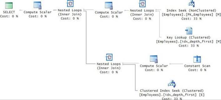
FIGURE 11-5 Execution plan for the custom materialized path subtree query.

The first Index Seek operator in the plan and the associated Key Lookup are in charge of retrieving the row for the filtered employee (empid 3). The second Index Seek operator in the plan performs a range scan in the index on the path attribute to retrieve the requested subtree of employees. Because the path attribute represents topological sorting, an index on path ensures that all members of the same subtree are stored contiguously in the leaf level of the index. Therefore, a request for a subtree is processed with a simple range scan in the index, touching only the nodes that, in fact, are members of the requested subtree.

To exclude the subtree’s root (top-level manager) from the output, simply add an underscore before the percent sign in the LIKE pattern:

With the additional underscore in the LIKE condition, an employee is returned only if its path starts with the root’s path and has at least one subsequent character.

To return leaf nodes under a given root (including the root itself if it is a leaf), add a NOT EXISTS predicate to identify only employees who are not managers of another employee:

SELECT E.empid, E.empname
FROM dbo.Employees AS E
INNER JOIN dbo.Employees AS M
ON M.empid = 3
AND E.path LIKE M.path + '%'
WHERE NOT EXISTS
(SELECT *
FROM dbo.Employees AS E2
WHERE E2.mgrid = E.empid);

empid empname
----------- --------
11 Gabriel
12 Emilia
13 Michael
14 Didi

To return a subtree with a given root, limiting the number of levels under the root, add a filter that limits the level difference between the employee and the root:

SELECT REPLICATE(' | ', E.lvl - M.lvl) + E.empname
FROM dbo.Employees AS E
INNER JOIN dbo.Employees AS M
ON M.empid = 3
AND E.path LIKE M.path + '%'
WHERE E.lvl - M.lvl <= 2
ORDER BY E.path;

Ina
| Aaron
| | Gabriel
| | Rita

To return only the nodes exactly n levels under a given root, use an equal to operator (=) to identify the specific level difference instead of a less than or equal to (<=) operator:

SELECT E.empid, E.empname
FROM dbo.Employees AS E
INNER JOIN dbo.Employees AS M
ON M.empid = 3
AND E.path LIKE M.path + '%'
WHERE E.lvl - M.lvl = 2;

empid empname
----------- --------
11 Gabriel
9 Rita

To return the management chain of a given node, you use a query similar to the subtree query, with one small difference: you filter a specific employee ID rather than filtering a specific manager ID:

You get all managers whose paths are a prefix of the given employee’s path.

Note that requesting a subtree and requesting the ancestors have an important difference in performance, even though they look very similar. For each query, either M.path or E.path is a constant. If M.path is constant, E.path LIKE M.path + ‘%’ enables the plan to use the index on pathefficiently, because the predicate asks for all paths with a given prefix and all qualifying rows appear in a consecutive section in the index. If E.path is constant, the plan does not use the index efficiently, because the predicate asks for all prefixes of a given path and all qualifying rows do not appear in a consecutive section in the index. The subtree query can seek within the index to the first path that meets the filter, and then perform a range scan until it gets to the last path that meets the filter. In other words, only the relevant paths in the index are accessed. Conversely, in the ancestors query, all paths must be scanned to check whether they match the filter. In large tables, this approach translates to a slow query. To handle ancestor requests more efficiently, you can create a function that accepts an employee ID as input, splits its path, and returns a table with the path’s node IDs in separate rows. You can join this table with the tree and use index seek operations for the specific employee IDs in the path. The split function uses the auxiliary table Nums from the sample database TSQLV3.

Run the following code to create the SplitPath function:

IF OBJECT_ID(N'dbo.SplitPath', N'IF') IS NOT NULL DROP FUNCTION dbo.SplitPath;
GO
CREATE FUNCTION dbo.SplitPath(@empid AS INT) RETURNS TABLE
AS
RETURN
SELECT ROW_NUMBER() OVER(ORDER BY n) AS pos,
CAST(SUBSTRING(path, n + 1, CHARINDEX('.', path, n + 1) - n - 1) AS INT) AS empid
FROM dbo.Employees
INNER JOIN TSQLV3.dbo.Nums
ON empid = @empid
AND n < LEN(path)
AND SUBSTRING(path, n, 1) = '.';
GO

You can find details on the logic behind the split technique that the function implements in Chapter 3, “Multi-table queries.”

To test the function, run the following code, which splits employee 14’s path:

SELECT pos, empid FROM dbo.SplitPath(14);

This code generates the following output:

pos empid
---- ------
1 1
2 3
3 7
4 9
5 14

To get the management chain of a given employee, join the table returned by the function with the Employees table, like so:

SELECT REPLICATE(' | ', lvl) + empname
FROM dbo.SplitPath(14) AS SP
INNER JOIN dbo.Employees AS E
ON E.empid = SP.empid
ORDER BY path;

When presenting information from a tree or a subtree, a common need is to present the nodes in topological sort order (parent before child). Because the path column already gives you topological sorting, you can simply sort the rows by path. Having an index on the path column means that the optimizer can satisfy the request with an index order scan as opposed to needing to apply a sort operation. As shown earlier, the indentation of nodes can be achieved by replicating a string lvl times. For example, the following query presents the employees in topological sort order:

SELECT REPLICATE(' | ', lvl) + empname
FROM dbo.Employees
ORDER BY path;

This code generates the following output:

The execution plan for this query is shown in Figure 11-6. Notice that the clustered index created on the path column is scanned in an ordered fashion.

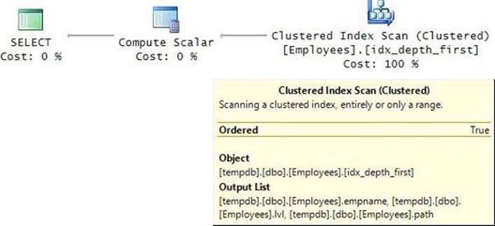
FIGURE 11-6 Execution plan for a custom materialized path sorting query.

Materialized path with the HIERARCHYID data type

SQL Server supports a CLR-based data type called HIERARCHYID that you can use to represent graphs. This type provides a built-in implementation for the materialized path model. Like the custom materialized path model, it works ideally for trees. As with the custom model, the HIERARCHYID values provide topological ordering, positioning a node in a certain place in the tree with respect to other nodes. Besides providing topological sorting, the HIERARCHYID paths position each node under a certain path of ancestors and in a certain place with respect to siblings. The HIERARCHYID paths differ from the custom model’s paths in two main ways. First, the custom model’s paths are made of the actual node IDs, whereas the HIERARCHYID paths are made of internally generated values. Second, the custom model’s path is character based, whereas the HIERARCHYID paths are binary. One of the major benefits I found with the HIERARCHYID type paths is that they tend to be more economical compared to the custom model’s paths. The encoding of the paths in the HIERARCHYID data type cannot exceed 892 bytes, but this limit shouldn’t present a problem for most trees. Also, you typically want to index the paths, sometimes adding other columns to the key list, and index keys are limited to 900 bytes anyway.

Note

The HIERARCHYID data type is a proprietary feature in SQL Server. If you care about the portability of your solution, you might prefer to stick to the custom model. That’s because it relies on basic language elements that are supported by virtually all SQL-based dialects: a character string column, an integer column, and the LIKE predicate. Still, it is worthwhile to be familiar with the HIERARCHYID data type for two main reasons:

1. You might need to maintain existing solutions that already use it.

2. There are features in SQL Server that use this data type, like the FileTable feature.

The HIERARCHYID type provides the following set of methods and properties that help you maintain and query the tree: GetLevel, GetRoot, GetAncestor, GetDescendant, GetReparentedValue, IsDescendantOf, ToString, Parse, Read, and Write. I will describe the methods and properties in the context of the tasks where they need to be used.

Note

I should mention several points about working with the HIERARCHYID type in terms of case sensitivity.

As a T-SQL type identifier, HIERARCHYID is always case insensitive, like any T-SQL keyword.

The method names associated with this type, like GetAncestor(), are always case sensitive, like any CLR identifier, whether they are static methods or not.

HIERARCHYID/hierarchyid, when used to identify the CLR class of a static method, as in hierarchyid::GetRoot(), is case sensitive or case insensitive according to the current database context. When the current database is case sensitive, lowercase must be used to identify the CLR class of a static method.

I chose to write the T-SQL type as HIERARCHYID for typographical reasons, but lowercase hierarchyid is the most portable choice for code.

Like I did with the custom model, I will use an employee organizational chart to demonstrate working with the HIERARCHYID type. Run the following code to create the Employees table, along with indexes similar to the ones used in the custom model to support typical queries:

IF OBJECT_ID(N'dbo.Employees', N'U') IS NOT NULL DROP TABLE dbo.Employees;
GO
CREATE TABLE dbo.Employees
(
empid INT NOT NULL,
hid HIERARCHYID NOT NULL,
lvl AS hid.GetLevel() PERSISTED,
empname VARCHAR(25) NOT NULL,
salary MONEY NOT NULL
);

CREATE UNIQUE CLUSTERED INDEX idx_depth_first ON dbo.Employees(hid);
CREATE UNIQUE INDEX idx_breadth_first ON dbo.Employees(lvl, hid);
ALTER TABLE dbo.Employees ADD CONSTRAINT PK_Employees PRIMARY KEY NONCLUSTERED(empid);

In addition to the hid column that holds the path, the table has a computed persisted column based on the GetLevel method applied to the hid column. As its name implies, the method returns the level of the node in the tree—in other words, the distance from the root.

As a reminder, besides the obvious index on the empid column that supports queries requesting a particular employee, the code creates two other indexes. It creates one for depth-first requests like returning a subtree, and presenting the nodes in topological sort order. It also creates another one for breadth-first requests like returning an entire level.

Notice that the Employees table does not include an attribute for the manager ID. With the HIERARCHYID type, you can easily address requests that would normally require such an attribute. Consequently, there’s no need for a self-referencing foreign key either.

Maintaining data

Whenever you need to apply changes to the tree, such as adding new leaf nodes or moving a subtree, you want to make sure you produce new HIERARCHYID values or adjust existing ones correctly. The HIERARCHYID type’s methods and properties can help you with such tasks. Also, note that the type itself does not enforce the validity of your tree—that’s your responsibility. For example, if you do not enforce the uniqueness of the HIERARCHYID values with a constraint, the type itself won’t reject attempts to insert multiple rows with the same HIERARCHYID value. Also, it is your responsibility to develop a process that prevents concurrent sessions that perform tree maintenance tasks from producing conflicting (the same) HIERARCHYID values for different nodes. I will explain how this can be achieved.

I will demonstrate techniques for adding employees who manage no one (leaf nodes) and for moving a subtree. I’ll leave other tasks—such as dropping a subtree and changing a manager—as exercises because those apply similar techniques to the ones I will cover.

Adding employees

The task of adding a new employee who manages no one requires you to produce a HIERARCHYID value for the new node that positions it correctly within the tree and then insert the new employee row into the table. Run the following code to create a stored procedure called AddEmp that implements this task:

The procedure accepts as inputs all attributes of the new employee (employee ID, manager ID, employee name, and salary). It then applies logic to generate the HIERARCHYID value of the new employee and store it in the variable @hid. Finally, the procedure uses the new HIERARCHYID value, @hid, in the new row it inserts into the Employees table.

The procedure’s code first checks whether the input employee is the root employee (that is, manager ID is NULL). In such a case, the code calculates the employee’s path with the static method hierarchyid::GetRoot. As you can imagine, the purpose of this method is to produce the path for the tree’s root node. In terms of the binary value that actually represents the path, this method simply returns an empty binary string (0x). You could, if you wanted, replace the static method call with the constant 0x, but with the method call the code is clearer and more self-explanatory.

The next section of the procedure’s code (the ELSE block of the IF statement) handles an input employee that is not the root employee. To calculate a path for an employee that is not the root employee, you can invoke the GetDescendant method applied to the HIERARCHYID value of the employee’s manager. The code retrieves the manager’s HIERARCHYID value, puts it into the @mgr_hid variable, and later applies the GetDescendant method to it.

The GetDescendant method accepts two input HIERARCHYID values and returns a HIERARCHYID value that is positioned under the node it is applied to and between the input left and right nodes. If both inputs are NULL, the method simply generates a value below the parent node. If the left input is not NULL, the method generates a value greater than the left input. If the right input is not NULL, the method generates a value less than the right input. Note that the method has no knowledge of other values in your tree; all it cares about is the value to which it is applied and the two input values. If you call the method twice and in both cases apply it to the same value with the same inputs, you get the same output back. It is your responsibility to prevent such conflicts.

A simple technique to achieve this is to run the code in a transaction (as in the AddEmp procedure) and specify the UPDLOCK hint in the query that retrieves the manager’s path. Remember that an update lock can be held by only one process on the same resource at a time. This hint allows only one session to request a new HIERARCHYID value under the same manager. This simple technique will guarantee that distinct HIERARCHYID values are generated by each process.

You need to be specific about where to position the new node with respect to other siblings under the same manager. For example, the inputs to the stored procedure could be the IDs of two employees between which you want to position the new employee, and the stored procedure could retrieve their HIERARCHYID values and provide those as the left and right values to the GetDescendant method. For this implementation, I decided that I’ll simply position the new employee right after the last child under the target manager. This strategy, coupled with the use of the UPDLOCK described earlier, is always safe in the sense that HIERARCHYID values of employees will never conflict. If you choose to implement a solution that allows specifying the left and right employees, the responsibility to prevent conflicts is now yours.

To apply my chosen strategy, immediately after a query that retrieves the path of the target manager, another query retrieves the maximum path among the existing subordinates of the manager, and the result is stored in the @last_child_hid variable. The method GetAncestor helps identify direct subordinates of the target manager. The method is applied to a HIERARCHYID value of a node, and it returns the HIERARCHYID value of an ancestor that is n levels up, where n is provided as input. For n=1, you get the node’s parent. So all employees for whom GetAncestor(1)returns the path of the manager are direct subordinates of the manager.

Once you have the path of the manager stored in the @mgr_hid variable and the path of the manager’s last direct subordinate is stored in the variable @last_child_hid, you can generate the input employee’s path with the expression @hid.GetDescendant(@last_child_hid, NULL). Once the path for the input employee is generated, you can insert the employee’s row into the Employees table and commit the transaction. Committing the transaction releases the update lock held on the manager’s row, allowing those who want to add other subordinates under that manager to generate new HIERARCHYID values.

Run the following code to populate the Employees table with sample data:

EXEC dbo.AddEmp @empid = 1, @mgrid = NULL, @empname = 'David' , @salary = $10000.00;
EXEC dbo.AddEmp @empid = 2, @mgrid = 1, @empname = 'Eitan' , @salary = $7000.00;
EXEC dbo.AddEmp @empid = 3, @mgrid = 1, @empname = 'Ina' , @salary = $7500.00;
EXEC dbo.AddEmp @empid = 4, @mgrid = 2, @empname = 'Seraph' , @salary = $5000.00;
EXEC dbo.AddEmp @empid = 5, @mgrid = 2, @empname = 'Jiru' , @salary = $5500.00;
EXEC dbo.AddEmp @empid = 6, @mgrid = 2, @empname = 'Steve' , @salary = $4500.00;
EXEC dbo.AddEmp @empid = 7, @mgrid = 3, @empname = 'Aaron' , @salary = $5000.00;
EXEC dbo.AddEmp @empid = 8, @mgrid = 5, @empname = 'Lilach' , @salary = $3500.00;
EXEC dbo.AddEmp @empid = 9, @mgrid = 7, @empname = 'Rita' , @salary = $3000.00;
EXEC dbo.AddEmp @empid = 10, @mgrid = 5, @empname = 'Sean' , @salary = $3000.00;
EXEC dbo.AddEmp @empid = 11, @mgrid = 7, @empname = 'Gabriel', @salary = $3000.00;
EXEC dbo.AddEmp @empid = 12, @mgrid = 9, @empname = 'Emilia' , @salary = $2000.00;
EXEC dbo.AddEmp @empid = 13, @mgrid = 9, @empname = 'Michael', @salary = $2000.00;
EXEC dbo.AddEmp @empid = 14, @mgrid = 9, @empname = 'Didi' , @salary = $1500.00;

Run the following query to present the contents of the Employees table:

SELECT hid, hid.ToString() AS path, lvl, empid, empname, salary
FROM dbo.Employees
ORDER BY hid;

The ToString method returns a canonical representation of the path, using slashes to separate the values at each level. This query generates the following output:

hid path lvl empid empname salary
--------- ---------- ------ ------ -------- ---------
0x / 0 1 David 10000.00
0x58 /1/ 1 2 Eitan 7000.00
0x5AC0 /1/1/ 2 4 Seraph 5000.00
0x5B40 /1/2/ 2 5 Jiru 5500.00
0x5B56 /1/2/1/ 3 8 Lilach 3500.00
0x5B5A /1/2/2/ 3 10 Sean 3000.00
0x5BC0 /1/3/ 2 6 Steve 4500.00
0x68 /2/ 1 3 Ina 7500.00
0x6AC0 /2/1/ 2 7 Aaron 5000.00
0x6AD6 /2/1/1/ 3 9 Rita 3000.00
0x6AD6B0 /2/1/1/1/ 4 12 Emilia 2000.00
0x6AD6D0 /2/1/1/2/ 4 13 Michael 2000.00
0x6AD6F0 /2/1/1/3/ 4 14 Didi 1500.00
0x6ADA /2/1/2/ 3 11 Gabriel 3000.00

This output gives you a sense of the logic that the GetDescendant method applies to calculate the values. The root (empty binary string) is represented by the canonical path /. The first child under a node obtains its HIERARCHYID from a call to GetDescendant with two NULL inputs. The result is the parent’s canonical path plus 1/. So the path of the first child of the root becomes /1/.

If you add someone to the right of an existing child and under that child’s parent, the new child’s hid is obtained by a call to GetDescendant with the existing child’s hid as the left input and NULL as the right input. The new path value is like the existing child’s value but with a rightmost number that is greater by one. So, for example, the value under / and to the right of /1/ would be /2/. Similarly, the value under /1/ and to the right of /1/1/ would be /1/2/.

If you add someone under a certain parent and to the left of an existing child, the left input to GetDescendant is NULL, and the new path value will be like the existing child’s but with a rightmost number that is less by one. So, for example, the value under /1/ and to the left of /1/1/ would be /1/0/. Similarly, the value under /1/ and to the left of /1/0/ would be /1/–1/.

If you add someone under a certain parent and provide two of that parent’s existing children’s hid values as inputs to GetDescendant, the resulting path matches the existing children’s paths except for the last number. If the last numbers in the existing children’s paths aren’t consecutive, the last number of the new child’s path will be one greater than that of the left child. For example, when the method is applied to the parent /1/1/ and the input children are /1/1/1/ and /1/1/4/, you get /1/1/2/. If the last path numbers of the input children are consecutive, you get the last number of the left child, followed by .1 (read “dot one”). For example, when the method is applied to the parent /1/1/ and the input children’s paths are /1/1/1/ and /1/1/2/, you get /1/1/1.1/. Similarly, when the method is applied to the parent /1/2.1/3/4/5/ and the input children are /1/2.1/3/4/5/2.1.3.4/ and /1/2.1/3/4/5/2.1.3.5/, you get /1/2.1/3/4/5/2.1.3.4.1/, and so on. As you might realize, the paths are simpler and shorter if you add new nodes either to the right of the last child or to the left of the first child.

Later in the chapter, in the section “Normalizing HIERARCHYID values,” I’ll explain how you can normalize paths when they become too lengthy.

Moving a subtree

The HIERARCHYID type supports a method called GetReparentedValue that helps in calculating new paths when you need to move a whole subtree to a new location in the tree. The method is applied to the HIERARCHYID value of a node that you want to reparent, but it doesn’t perform the actual reparenting. It simply returns a new value you can then use to overwrite the existing path. The method accepts two inputs (call them @old_root and @new_root) and returns a new value with the target node’s path where the @new_root prefix replaces the @old_root prefix. It’s as simple as that.

Note

When you call GetReparentedValue on a HIERARCHYID h, the path of @old_root must be a prefix of h’s path. If it is not, you’ll get an exception of type HierarchyIdException.

For example, if you apply the GetReparentedValue method to a HIERARCHYID whose canonical path is /1/1/2/3/2/, providing /1/1/ as the old root and /2/1/4/ as the new root, you get a HIERARCHYID whose canonical path is /2/1/4/2/3/2/. By the way, you can cast a canonical path representation to the HIERARCHYID data type by using the CAST function or the static method hierarchyid::Parse. You can test the aforementioned example by using the GetReparentedValue with constants, like so:

SELECT CAST('/1/1/2/3/2/' AS HIERARCHYID).GetReparentedValue('/1/1/', '/2/1/4/').ToString();

You get the path /2/1/4/2/3/2/ as output.

With this in mind, consider the task to create a stored procedure called MoveSubtree that accepts two inputs called @empid and @new_mgrid. The stored procedure’s purpose is to move the subtree of employee @empid under @new_mgrid. The stored procedure can implement the task in three steps:

1. Store the existing paths of the employees represented by @new_mgrid and @empid in variables. (Call them @new_mgr_hid and @old_root, respectively.)

2. Apply the GetDescendant method to @new_mgr_hid, providing the maximum among the new manager’s existing subordinates (or NULL if there are none) as left input, to get a new path under the target manager for employee @empid. Store the new path in a variable. (Call it@new_root.)

3. Update the hid value of all descendants of the employee represented by @empid (including itself) to hid.GetReparentedValue(@old_root, @new_root). To identify all descendants of a node, you can check the value of the method IsDescendantOf on each hid in the table. This method returns 1 when the node it is applied to is a descendant of the input node and 0 otherwise.

Run the following code to create the MoveSubtree stored procedure, which implements the preceding steps:

---------------------------------------------------------------------
-- Stored Procedure: MoveSubtree,
-- Moves a whole subtree of a given root to a new location
-- under a given manager
---------------------------------------------------------------------
IF OBJECT_ID(N'dbo.MoveSubtree', N'P') IS NOT NULL DROP PROC dbo.MoveSubtree;
GO
CREATE PROC dbo.MoveSubtree
@empid AS INT,
@new_mgrid AS INT
AS

DECLARE
@old_root AS HIERARCHYID,
@new_root AS HIERARCHYID,
@new_mgr_hid AS HIERARCHYID;

BEGIN TRAN

SET @new_mgr_hid = (SELECT hid FROM dbo.Employees WITH (UPDLOCK)
WHERE empid = @new_mgrid);
SET @old_root = (SELECT hid FROM dbo.Employees
WHERE empid = @empid);

-- First, get a new hid for the subtree root employee that moves
SET @new_root = @new_mgr_hid.GetDescendant
((SELECT MAX(hid)
FROM dbo.Employees
WHERE hid.GetAncestor(1) = @new_mgr_hid),
NULL);

-- Next, reparent all descendants of employee that moves
UPDATE dbo.Employees
SET hid = hid.GetReparentedValue(@old_root, @new_root)
WHERE hid.IsDescendantOf(@old_root) = 1;

COMMIT TRAN
GO

Notice that the code uses an explicit transaction, and as the first step when querying the target manager’s row, the statement obtains an update lock on that row. Much like in the AddEmp procedure discussed earlier, this technique guarantees that only one subtree is moved under a given target manager at a time, which prevents conflicts in the newly generated HIERARCHYID values.

To test the MoveSubtree procedure, run the following code, moving the subtree of employee 5 (Jiru) under employee 9 (Rita):

SELECT empid, REPLICATE(' | ', lvl) + empname AS empname, hid.ToString() AS path
FROM dbo.Employees
ORDER BY hid;

BEGIN TRAN

EXEC dbo.MoveSubtree
@empid = 5,
@new_mgrid = 9;

SELECT empid, REPLICATE(' | ', lvl) + empname AS empname, hid.ToString() AS path
FROM dbo.Employees
ORDER BY hid;

ROLLBACK TRAN

The code presents the before and after states of the data, and because this is just a demonstration, it runs the activity in a transaction so that the changes won’t be committed. Following are the outputs of this code showing that the subtree was moved correctly:

Querying

As with the custom materialized path solution, querying data in the built-in materialized path solution that is based on the HIERARCHYID data type is simple and elegant. With the depth-first and breadth-first indexes in place, you can enable SQL Server’s optimizer to handle certain types of requests efficiently.

I won’t cover all possible requests against the tree here because there are so many. Instead, I’ll show a sample of the common ones. As I did before, I’ll provide a sample query for each request followed by its output.

Subgraph/descendants

Return the subtree of employee 3, limiting the number of levels under the input employee to 3:

SELECT E.empid, E.empname
FROM dbo.Employees AS M
INNER JOIN dbo.Employees AS E
ON M.empid = 3
AND E.hid.IsDescendantOf(M.hid) = 1
WHERE E.lvl - M.lvl <= 3;

The query uses the IsDescendantOf method. Recall that this method returns 1 if the node to which it is applied is a descendant of the input node and 0 otherwise. The query joins two instances of the Employees table: one representing the input manager (M) and one representing the subordinates (E). The predicate in the ON clause filters only one row from the instance M—the one for employee 3—and returns all employees from E that are descendants of the employee in M. The predicate in the WHERE clause filters only employees that are up to three levels below the employee in M.

This query generates the following output:

empid empname
----------- -------------------------
3 Ina
7 Aaron
9 Rita
12 Emilia
13 Michael
14 Didi
11 Gabriel

The execution plan of this query is shown in Figure 11-7.

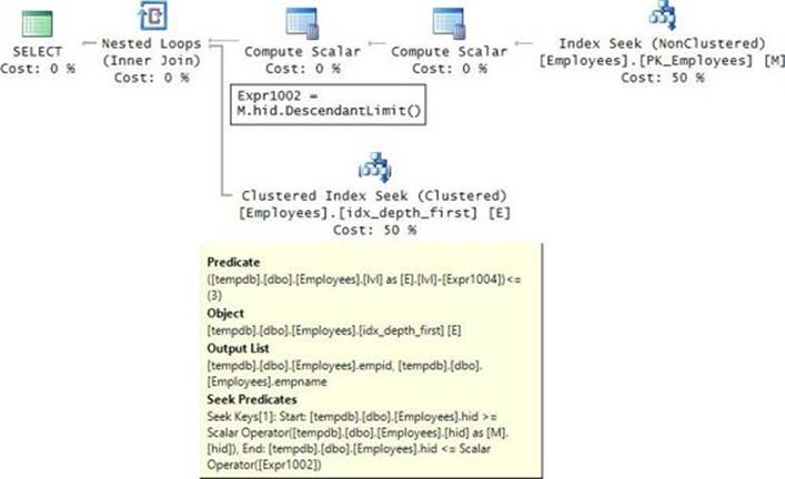
FIGURE 11-7 Execution plan for a HIERARCHYID subtree query.

The first Index Seek operator in the plan (the top one) is responsible for returning the row for employee 3 from the index on the empid column. A Compute Scalar operator (the second one) then calculates the upper boundary point of the HIERARCHYID values of the requested subtree by invoking an internal method called DescendantLimit, storing the result in the variable Expr1002. Recall that because the HIERARCHYID values give you topological sorting, an index on the hid column arranges all members of the same subtree together. The second Index Seek operator in the plan (the bottom one) performs a range scan in the index on hid based on the predicate: E.hid >= M.hid AND E.hid <= Expr1002. This plan is pretty much as good as it can get for this kind of request because SQL Server ends up scanning only the members of the applicable subtree.

Ancestors/path

Next, I’ll explain how to handle a request to return all managers in the path leading to a certain employee. You can implement a solution that is similar to the one used to handle the subtree request. Instead of filtering the row representing the one manager (from an instance M of Employees) and then returning the attributes of all qualifying subordinates (from an instance E), you filter the row representing the one employee and then return the attributes of all qualifying managers. For example, the following query returns all managers of employee 14, direct or indirect:

SELECT M.empid, M.empname
FROM dbo.Employees AS M
INNER JOIN dbo.Employees AS E
ON E.empid = 14
AND E.hid.IsDescendantOf(M.hid) = 1;

This query generates the following output:

empid empname
----------- -------------------------
1 David
3 Ina
7 Aaron
9 Rita
14 Didi

Although this query is similar to the one that implemented the subtree request, it cannot be optimized as efficiently. That’s because members of the same path do not reside in a consecutive range in the index.

Children/direct subordinates

Next, I’ll describe how to handle a request to get direct subordinates of an employee. To handle this request, you can use a similar join form as in the previous queries. Filter the one row representing the employee whose subordinates you want from an instance (M) of the Employees table and return all employees (from another instance, E) whose parent is the employee filtered from M. A node’s parent is its ancestor one level up, and the GetAncestor method with input value 1 returns the parent HIERARCHYID value. As an example of finding direct subordinates, the following query returns direct subordinates of employee 2:

SELECT E.empid, E.empname
FROM dbo.Employees AS M
INNER JOIN dbo.Employees AS E
ON M.empid = 2
AND E.hid.GetAncestor(1) = M.hid;

This code generates the following output:

empid empname
----------- -------------------------
4 Seraph
5 Jiru
6 Steve

Leaf nodes

You can also use the GetAncestor method with input value 1 to identify leaf nodes. Leaf nodes, or employees who manage no one, are employees that do not appear as the parent of other employees. This logic can be implemented with a NOT EXISTS predicate, like so:

SELECT empid, empname
FROM dbo.Employees AS M
WHERE NOT EXISTS
(SELECT * FROM dbo.Employees AS E
WHERE E.hid.GetAncestor(1) = M.hid);

This code generates the following output:

empid empname
----------- -------------------------
4 Seraph
8 Lilach
10 Sean
6 Steve
12 Emilia
13 Michael
14 Didi
11 Gabriel

Presentation

Finally, to present the hierarchy of employees so that a subordinate appears under and to the right of its manager, use the following query:

SELECT REPLICATE(' | ', lvl) + empname AS empname, hid.ToString() AS path
FROM dbo.Employees
ORDER BY hid;

Recall that the HIERARCHYID data type gives you topological sorting, so all you need to do to get the desired presentation ordering is to order by the hid attribute. Indentation is achieved by replicating a string lvl times. This query generates the following output:

The execution plan of this query is shown in Figure 11-8.

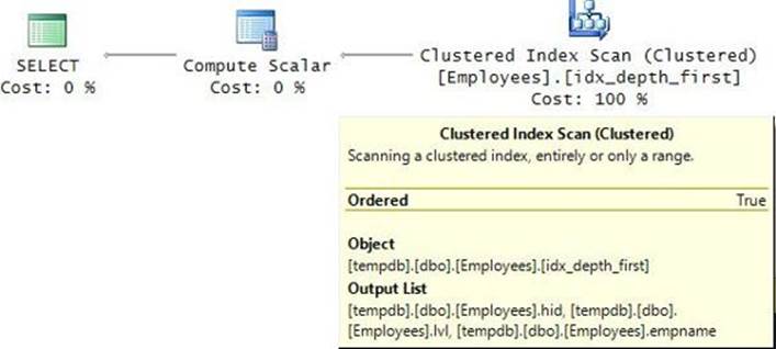
FIGURE 11-8 Execution plan for a HIERARCHYID sorting query.

You can see that the optimizer efficiently processed the request with an ordered scan of the index on the hid column.

Further aspects of working with HIERARCHYID

This section covers further aspects of working with the HIERARCHYID data type. I’ll explain the circumstances in which paths can get lengthy and provide you with a solution to normalize them. I’ll show you how to convert a representation of a tree as an adjacency list to one that is based on the HIERARCHYID data type. Finally, I’ll show you how you can use the HIERARCHYID data type to sort separated lists of values.

Normalizing HIERARCHYID values

When you use the HIERARCHYID data type to represent trees, in certain cases the paths can become long. With very deep trees, this is natural because the HIERARCHYID value represents a path of all nodes leading to the current node, starting with the root. However, in certain cases, even when the tree is not very deep, the path can become long. First I’ll explain the circumstances in which this can happen, and then I’ll provide a solution to normalizing the values, making them shorter. Note that in this section, the word normalizing does not refer to database normalization.

HIERARCHYID values can become long when you keep adding new nodes between existing nodes whose canonical paths have consecutive last numbers. For example, say you have nodes with canonical paths /1/ and /2/ and you add a node between them. You get a new value whose canonical path is /1.1/. Now add a value between /1.1/ and /2/, and you get /1.2/. Now add a value between /1.1/ and /1.2/, and you get /1.1.1/. As you see, if you keep adding nodes between existing nodes in this manner, you can get lengthy paths (which represent lengthy HIERARCHYID values) even when the tree is not deep.

If order among siblings is not important, you can always make sure to add new child nodes after the last existing child or before the first one; this way, the paths are more economical. But when order among siblings matters, you can’t control this. If you must frequently add new nodes between existing ones, you might end up with very long HIERARCHYID values. In such a case, you can periodically run a procedure, which I will provide here, that normalizes the HIERARCHYID values for the whole graph, making them shorter.

Run the following code to create a new version of the AddEmp stored procedure:

This version accepts the IDs of the two child employees between which you want to add the new one.

Next, run the following code, which truncates the Employees table and populates it with data in such a manner that lengthy paths are produced:

TRUNCATE TABLE dbo.Employees;

EXEC dbo.AddEmp @empid = 1, @mgrid = NULL, @leftempid = NULL, @rightempid = NULL,
@empname = 'A';
EXEC dbo.AddEmp @empid = 2, @mgrid = 1, @leftempid = NULL, @rightempid = NULL,
@empname = 'B';
EXEC dbo.AddEmp @empid = 3, @mgrid = 1, @leftempid = 2, @rightempid = NULL,
@empname = 'C';
EXEC dbo.AddEmp @empid = 4, @mgrid = 1, @leftempid = 2, @rightempid = 3,
@empname = 'D';
EXEC dbo.AddEmp @empid = 5, @mgrid = 1, @leftempid = 4, @rightempid = 3,
@empname = 'E';
EXEC dbo.AddEmp @empid = 6, @mgrid = 1, @leftempid = 4, @rightempid = 5,
@empname = 'F';
EXEC dbo.AddEmp @empid = 7, @mgrid = 1, @leftempid = 6, @rightempid = 5,
@empname = 'G';
EXEC dbo.AddEmp @empid = 8, @mgrid = 1, @leftempid = 6, @rightempid = 7,
@empname = 'H';
EXEC dbo.AddEmp @empid = 9, @mgrid = 8, @leftempid = NULL, @rightempid = NULL,
@empname = 'I';
EXEC dbo.AddEmp @empid = 10, @mgrid = 8, @leftempid = 9, @rightempid = NULL,
@empname = 'J';
EXEC dbo.AddEmp @empid = 11, @mgrid = 8, @leftempid = 9, @rightempid = 10,
@empname = 'K';
EXEC dbo.AddEmp @empid = 12, @mgrid = 8, @leftempid = 11, @rightempid = 10,
@empname = 'J';
EXEC dbo.AddEmp @empid = 13, @mgrid = 8, @leftempid = 11, @rightempid = 12,
@empname = 'L';
EXEC dbo.AddEmp @empid = 14, @mgrid = 8, @leftempid = 13, @rightempid = 12,
@empname = 'M';
EXEC dbo.AddEmp @empid = 15, @mgrid = 8, @leftempid = 13, @rightempid = 14,
@empname = 'N';
EXEC dbo.AddEmp @empid = 16, @mgrid = 8, @leftempid = 15, @rightempid = 14,
@empname = 'O';
EXEC dbo.AddEmp @empid = 17, @mgrid = 8, @leftempid = 15, @rightempid = 16,
@empname = 'P';
EXEC dbo.AddEmp @empid = 18, @mgrid = 8, @leftempid = 17, @rightempid = 16,
@empname = 'Q';
EXEC dbo.AddEmp @empid = 19, @mgrid = 8, @leftempid = 17, @rightempid = 18,
@empname = 'E';
EXEC dbo.AddEmp @empid = 20, @mgrid = 8, @leftempid = 19, @rightempid = 18,
@empname = 'S';
EXEC dbo.AddEmp @empid = 21, @mgrid = 8, @leftempid = 19, @rightempid = 20,
@empname = 'T';

Then run the following code to show the current HIERARCHYID values and their canonical paths:

SELECT empid, REPLICATE(' | ', lvl) + empname AS emp, hid, hid.ToString() AS path
FROM dbo.Employees
ORDER BY hid;

You get the following output:

empid emp hid path
------ -------- ----------------- -----------------------
1 A 0x /
2 | B 0x58 /1/
4 | D 0x62C0 /1.1/
6 | F 0x6316 /1.1.1/
8 | H 0x6318B0 /1.1.1.1/
9 | | I 0x6318B580 /1.1.1.1/1/
11 | | K 0x6318B62C /1.1.1.1/1.1/
13 | | L 0x6318B63160 /1.1.1.1/1.1.1/
15 | | N 0x6318B6318B /1.1.1.1/1.1.1.1/
17 | | P 0x6318B6318C58 /1.1.1.1/1.1.1.1.1/
19 | | E 0x6318B6318C62C0 /1.1.1.1/1.1.1.1.1.1/
21 | | T 0x6318B6318C6316 /1.1.1.1/1.1.1.1.1.1.1/
20 | | S 0x6318B6318C6340 /1.1.1.1/1.1.1.1.1.2/
18 | | Q 0x6318B6318C68 /1.1.1.1/1.1.1.1.2/
16 | | O 0x6318B6318D /1.1.1.1/1.1.1.2/
14 | | M 0x6318B631A0 /1.1.1.1/1.1.2/
12 | | J 0x6318B634 /1.1.1.1/1.2/
10 | | J 0x6318B680 /1.1.1.1/2/
7 | G 0x631A /1.1.2/
5 | E 0x6340 /1.2/
3 | C 0x68 /2/

As you can see, even though the tree is only three levels deep, some of the HIERARCHYID values became quite long because of the insertion order of children.

The solution that normalizes the values involves the following steps:

1. Define a CTE called EmpsRN that calculates for each node a row number, partitioned by parent and ordered by current hid value.

2. Define a recursive CTE called EmpPaths that iterates through the levels of the tree, starting with the root node and proceeding to the next level of children in each iteration. Use this CTE to construct a new canonical path for the nodes. The root should be assigned the path /, and for each node in the next level the path is obtained by concatenating the parent’s path, the current node’s row number from the previous step, and another / character.

3. Join the Employees table with the EmpPaths CTE, and update the existing hid values with new ones converted from the canonical paths generated in the previous step.

Here’s the code that performs this normalization process:

WITH EmpsRN AS
(
SELECT empid, hid, ROW_NUMBER() OVER(PARTITION BY hid.GetAncestor(1) ORDER BY hid) AS rownum
FROM dbo.Employees
),
EmpPaths AS
(
SELECT empid, hid, CAST('/' AS VARCHAR(900)) AS path
FROM dbo.Employees
WHERE hid = hierarchyid::GetRoot()

UNION ALL

SELECT C.empid, C.hid, CAST(P.path + CAST(C.rownum AS VARCHAR(20)) + '/' AS VARCHAR(900))
FROM EmpPaths AS P
INNER JOIN EmpsRN AS C
ON C.hid.GetAncestor(1) = P.hid
)
UPDATE E
SET hid = CAST(EP.path AS HIERARCHYID)
FROM dbo.Employees AS E
INNER JOIN EmpPaths AS EP
ON E.empid = EP.empid;

Now query the data after normalization:

SELECT empid, REPLICATE(' | ', lvl) + empname AS emp, hid, hid.ToString() AS path
FROM dbo.Employees
ORDER BY hid;

As you can see in the output, you get nice compact paths:

empid emp hid path
----------- -------- ------- -------
1 A 0x /
2 | B 0x58 /1/
4 | D 0x68 /2/
6 | F 0x78 /3/
8 | H 0x84 /4/
9 | | I 0x8560 /4/1/
11 | | K 0x85A0 /4/2/
13 | | L 0x85E0 /4/3/
15 | | N 0x8610 /4/4/
17 | | P 0x8630 /4/5/
19 | | E 0x8650 /4/6/
21 | | T 0x8670 /4/7/
20 | | S 0x8688 /4/8/
18 | | Q 0x8698 /4/9/
16 | | O 0x86A8 /4/10/
14 | | M 0x86B8 /4/11/
12 | | J 0x86C8 /4/12/
10 | | J 0x86D8 /4/13/
7 | G 0x8C /5/
5 | E 0x94 /6/
3 | C 0x9C /7/

Convert a parent-child representation to HIERARCHYID

This section explains how to convert an existing representation of a tree that is based on an adjacency list (parent-child relationships) to one that is based on the HIERARCHYID data type.

Run the following code to create and populate the EmployeesOld table that implements an adjacency-list representation of an employee tree:

IF OBJECT_ID(N'dbo.EmployeesOld', N'U') IS NOT NULL DROP TABLE dbo.EmployeesOld;
IF OBJECT_ID(N'dbo.EmployeesNew', N'U') IS NOT NULL DROP TABLE dbo.EmployeesNew;
GO
CREATE TABLE dbo.EmployeesOld
(
empid INT CONSTRAINT PK_EmployeesOld PRIMARY KEY,
mgrid INT NULL CONSTRAINT FK_EmpsOld_EmpsOld REFERENCES dbo.EmployeesOld,
empname VARCHAR(25) NOT NULL,
salary MONEY NOT NULL
);
CREATE UNIQUE INDEX idx_unc_mgrid_empid ON dbo.EmployeesOld(mgrid, empid);

INSERT INTO dbo.EmployeesOld(empid, mgrid, empname, salary) VALUES
(1, NULL, 'David', $10000.00),
(2, 1, 'Eitan', $7000.00),
(3, 1, 'Ina', $7500.00),
(4, 2, 'Seraph', $5000.00),
(5, 2, 'Jiru', $5500.00),
(6, 2, 'Steve', $4500.00),
(7, 3, 'Aaron', $5000.00),
(8, 5, 'Lilach', $3500.00),
(9, 7, 'Rita', $3000.00),
(10, 5, 'Sean', $3000.00),
(11, 7, 'Gabriel', $3000.00),
(12, 9, 'Emilia' , $2000.00),
(13, 9, 'Michael', $2000.00),
(14, 9, 'Didi', $1500.00);

Run the following code to create the target EmployeesNew table that will represent the employee tree using HIERARCHYID values:

CREATE TABLE dbo.EmployeesNew
(
empid INT NOT NULL,
hid HIERARCHYID NOT NULL,
lvl AS hid.GetLevel() PERSISTED,
empname VARCHAR(25) NOT NULL,
salary MONEY NOT NULL
);

The task is now to query the EmployeesOld table that contains the source data, calculate HIERARCHYID values for the employees, and populate the target EmployeesNew table. This task can be achieved in a similar manner to normalizing existing HIERARCHYID values as described earlier. You apply the following steps:

1. Define a CTE called EmpsRN that calculates for each node a row number partitioned by mgrid, ordered by the attributes that should determine order among siblings—for example, empid.

3. Insert into the target table EmployeesNew the employee rows along with their newly generated HIERARCHYID values from the EmpPaths CTE.

Here’s the code that performs this conversion process:

WITH EmpsRN AS
(
SELECT empid, mgrid, empname, salary,
ROW_NUMBER() OVER(PARTITION BY mgrid ORDER BY empid) AS rn
FROM dbo.EmployeesOld
),
EmpPaths AS
(
SELECT empid, mgrid, empname, salary,
CAST('/' AS VARCHAR(900)) AS cpath
FROM dbo.EmployeesOld
WHERE mgrid IS NULL

UNION ALL

SELECT C.empid, C.mgrid, C.empname, C.salary,
CAST(cpath + CAST(C.rn AS VARCHAR(20)) + '/' AS VARCHAR(900))
FROM EmpPaths AS P
INNER JOIN EmpsRN AS C
ON C.mgrid = P.empid
)
INSERT INTO dbo.EmployeesNew WITH (TABLOCK) (empid, empname, salary, hid)
SELECT empid, empname, salary, CAST(cpath AS HIERARCHYID) AS hid
FROM EmpPaths;

Run the following code to create the recommended indexes to support typical queries:

CREATE UNIQUE CLUSTERED INDEX idx_depth_first ON dbo.EmployeesNew(hid);
CREATE UNIQUE INDEX idx_breadth_first ON dbo.EmployeesNew(lvl, hid);
ALTER TABLE dbo.EmployeesNew ADD CONSTRAINT PK_EmployeesNew PRIMARY KEY NONCLUSTERED(empid);

Run the following code to present the contents of the EmployeesNew table after the conversion:

SELECT REPLICATE(' | ', lvl) + empname AS empname, hid.ToString() AS path
FROM dbo.EmployeesNew
ORDER BY hid;

You get the following output:

Sorting separated lists of values

Some applications store information about arrays and lists of numbers in the form of character strings with separated lists of values. I won’t get into a discussion here regarding whether such representation of data is really appropriate. Instead, I’ll address a certain need involving such representation. Sometimes you don’t have control over the design of certain systems, and you need to provide solutions to requests using the existing design.

The request at hand involves sorting such lists, but based on the numeric values of the elements and not by their character representation. For example, consider the lists ‘13,41,17’ and ‘13,41,3’. If you sort the lists based on the character representation of the elements, the former would be returned before the latter because the character ‘1’ is considered smaller than the character ‘3’. You want the second string to sort before the first because the number 3 is smaller than the number 17.

A special case of the problem is sorting IP addresses represented as character strings. In this special case, you have an assurance that each string always has exactly four elements, and the length of each element never exceeds three digits. I’ll first cover this special case and then discuss the more generic one.

Run the following code to create the IPs table, and populate it with some sample IP addresses:

IF OBJECT_ID(N'dbo.IPs', N'U') IS NOT NULL DROP TABLE dbo.IPs;
GO
-- Creation script for table IPs
CREATE TABLE dbo.IPs
(
ip varchar(15) NOT NULL,
CONSTRAINT PK_IPs PRIMARY KEY(ip),
-- CHECK constraint that validates IPs
CONSTRAINT CHK_IP_valid CHECK
(
-- 3 periods and no empty octets
ip LIKE '_%._%._%._%'
AND
-- not 4 periods or more
ip NOT LIKE '%.%.%.%.%'
AND
-- no characters other than digits and periods
ip NOT LIKE '%[^0-9.]%'
AND
-- not more than 3 digits per octet
ip NOT LIKE '%[0-9][0-9][0-9][0-9]%'
AND
-- NOT 300 - 999
ip NOT LIKE '%[3-9][0-9][0-9]%'
AND
-- NOT 260 - 299
ip NOT LIKE '%2[6-9][0-9]%'
AND
-- NOT 256 - 259
ip NOT LIKE '%25[6-9]%'
)
);
GO

-- Sample data
INSERT INTO dbo.IPs(ip) VALUES
('131.107.2.201'),
('131.33.2.201'),
('131.33.2.202'),
('3.107.2.4'),
('3.107.3.169'),
('3.107.104.172'),
('22.107.202.123'),
('22.20.2.77'),
('22.156.9.91'),
('22.156.89.32');

I’ll first describe one of the solutions I had for this need without using the HIERARCHYID data type.

An IP address must be one of 81 (3⁴) possible patterns in terms of the number of digits in each octet (assuming we are talking about IPv4). You can write a query that produces all possible patterns that a LIKE predicate would recognize, representing each digit with an underscore. You can use an auxiliary table of numbers (like the Nums table in the TSQLV3 database) that has three numbers for the three possible octet lengths. By joining four instances of the Nums table, you get the 81 possible variations of the four octet sizes. You can then construct the LIKE patterns representing the IP addresses and, using the numbers from the Nums table, calculate the starting position and length of each octet.

Run the following code to create and query the view IPPatterns, which implements this logic:

IF OBJECT_ID(N'dbo.IPPatterns', N'V') IS NOT NULL DROP VIEW dbo.IPPatterns;
GO
CREATE VIEW dbo.IPPatterns
AS

SELECT
REPLICATE('_', N1.n) + '.' + REPLICATE('_', N2.n) + '.'
+ REPLICATE('_', N3.n) + '.' + REPLICATE('_', N4.n) AS pattern,
N1.n AS l1, N2.n AS l2, N3.n AS l3, N4.n AS l4,
1 AS s1, N1.n+2 AS s2, N1.n+N2.n+3 AS s3, N1.n+N2.n+N3.n+4 AS s4
FROM TSQLV3.dbo.Nums AS N1 CROSS JOIN TSQLV3.dbo.Nums AS N2
CROSS JOIN TSQLV3.dbo.Nums AS N3 CROSS JOIN TSQLV3.dbo.Nums AS N4
WHERE N1.n <= 3 AND N2.n <= 3 AND N3.n <= 3 AND N4.n <= 3;
GO

SELECT pattern, l1, l2, l3, l4, s1, s2, s3, s4 FROM dbo.IPPatterns;

When you query the view, you get the possible IP patterns and the starting position and length of each pattern, as shown here in abbreviated form:

pattern l1 l2 l3 l4 s1 s2 s3 s4
--------------- --- --- --- --- --- --- --- ---
_._._._ 1 1 1 1 1 3 5 7
_._._.__ 1 1 1 2 1 3 5 7
_._._.___ 1 1 1 3 1 3 5 7
_._.__._ 1 1 2 1 1 3 5 8
_._.__.__ 1 1 2 2 1 3 5 8
_._.__.___ 1 1 2 3 1 3 5 8
_._.___._ 1 1 3 1 1 3 5 9
_._.___.__ 1 1 3 2 1 3 5 9
_._.___.___ 1 1 3 3 1 3 5 9
_.__._._ 1 2 1 1 1 3 6 8
_.__._.__ 1 2 1 2 1 3 6 8
_.__._.___ 1 2 1 3 1 3 6 8
_.__.__._ 1 2 2 1 1 3 6 9
_.__.__.__ 1 2 2 2 1 3 6 9
_.__.__.___ 1 2 2 3 1 3 6 9
_.__.___._ 1 2 3 1 1 3 6 10
_.__.___.__ 1 2 3 2 1 3 6 10
_.__.___.___ 1 2 3 3 1 3 6 10
_.___._._ 1 3 1 1 1 3 7 9
_.___._.__ 1 3 1 2 1 3 7 9
...

Of course, you can implement similar logic to create the possible patterns for IP addresses of IPv6.

Now you can write a query that joins the IPs table with the IPPatterns view based on a match between the IP address and the IP pattern. This way you identify the IP pattern for each IP address, along with the measures indicating the starting position and length of each octet. You can then specify four expressions in the ORDER BY clause that apply the SUBSTRING function to extract the octets and cast the character-string representation of the octet to a numeric one. Here’s what the query looks like:

SELECT ip
FROM dbo.IPs
INNER JOIN dbo.IPPatterns
ON ip LIKE pattern
ORDER BY
CAST(SUBSTRING(ip, s1, l1) AS TINYINT),
CAST(SUBSTRING(ip, s2, l2) AS TINYINT),
CAST(SUBSTRING(ip, s3, l3) AS TINYINT),
CAST(SUBSTRING(ip, s4, l4) AS TINYINT);

This query generates the following output:

ip
---------------
3.107.2.4
3.107.3.169
3.107.104.172
22.20.2.77
22.107.202.123
22.156.9.91
22.156.89.32
131.33.2.201
131.33.2.202
131.107.2.201

The problem with this solution is that it’s not very efficient, and it doesn’t work in the more generic cases of lists where you have an unknown number of elements.

Interestingly, the canonical representation of HIERARCHYID values is also a separated list of numbers. Within a level, you can have values separated by dots, and between levels the values are separated by slashes. With this in mind, you can handle the task at hand by concatenating a slash before and after the IP address, and then sorting the rows after converting the result to the HIERARCHYID data type, like so:

SELECT ip
FROM dbo.IPs
ORDER BY CAST('/' + ip + '/' AS HIERARCHYID);

This solution works just as well with the more generic case of the problem. To demonstrate this, first create and populate the table T1 by running the following code:

IF OBJECT_ID(N'dbo.T1', N'U') IS NOT NULL DROP TABLE dbo.T1;
GO
CREATE TABLE dbo.T1
(
id INT NOT NULL IDENTITY PRIMARY KEY,
val VARCHAR(500) NOT NULL
);

INSERT INTO dbo.T1(val) VALUES
('100'),
('7,4,250'),
('22,40,5,60,4,100,300,478,19710212'),
('22,40,5,60,4,99,300,478,19710212'),
('22,40,5,60,4,99,300,478,9999999'),
('10,30,40,50,20,30,40'),
('7,4,250'),
('-1'),
('-2'),
('-11'),
('-22'),
('-123'),
('-321'),
('22,40,5,60,4,-100,300,478,19710212'),
('22,40,5,60,4,-99,300,478,19710212');

As you can see, the lists in the table have varying numbers of elements. Note that because the separator used in these lists is a comma, you need to replace the separators by slashes or dots before converting to the HIERARCHYID data type. Here’s the solution query that sorts the lists by the numeric values of the elements:

SELECT id, val
FROM dbo.T1
ORDER BY CAST('/' + REPLACE(val, ',', '/') + '/' AS HIERARCHYID);

This query generates the following output:

id val
----------- ------------------------------------
13 -321
12 -123
11 -22
10 -11
9 -2
8 -1
7 7,4,250
2 7,4,250
6 10,30,40,50,20,30,40
14 22,40,5,60,4,-100,300,478,19710212
15 22,40,5,60,4,-99,300,478,19710212
5 22,40,5,60,4,99,300,478,9999999
4 22,40,5,60,4,99,300,478,19710212
3 22,40,5,60,4,100,300,478,19710212
1 100

Note that you can create a computed persisted column in the table based on this expression and index that column. Such an index can support a request to sort the data without the need for an explicit sort operation in the query’s execution plan.

Nested sets

The nested sets solution is one of the most beautiful solutions I’ve seen for modeling trees.

More Info

Joe Celko has extensive coverage of the nested sets model in his writings. You can find Joe Celko’s coverage of nested sets in his book Joe Celko’s Trees and Hierarchies in SQL for Smarties, Second Edition (Morgan Kaufmann, 2012).

The main advantages of the nested sets solution are simple and fast queries, which I’ll describe later, and no level limit. Unfortunately, however, with large data sets the solution’s practicality is usually limited to static trees. For dynamic environments that incur frequent changes, the solution is limited to small trees (or forests of small trees).

Instead of representing a tree as an adjacency list (parent-child relationship), this solution models the tree relationships as nested sets. A parent is represented in the nested sets model as a containing set, and a child is represented as a contained set. Set containment relationships are represented with two integer values assigned to each set: left and right. For all sets, a set’s left value is smaller than all contained sets’ left values, and a set’s right value is higher than all contained sets’ right values. Naturally, this containment relationship is transitive in terms of n-level relationships (ancestor/descendant). The queries are based on these nested sets relationships. Logically, it’s as if a set spreads two arms around all its contained sets.

Assigning left and right values

Figure 11-9 provides a graphical visualization of the Employees tree with the left and right values assigned to each employee.

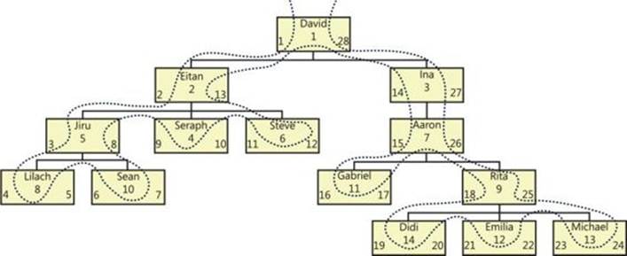
FIGURE 11-9 Employees hierarchy as nested sets.

The curved line that walks the tree represents the order of assignment of the left and right values. Note that the model allows you to choose in which order you assign values to siblings. In this particular case, I chose to traverse siblings by employee name order.

You start with the root, traversing the tree counterclockwise. Every time you enter a node, you increment a counter and set it as the node’s left value. Every time you leave a node, you increment the counter and set it as the node’s right value. This algorithm can be implemented to the letter as an iterative or recursive routine that assigns each node with left and right values. However, such an implementation requires traversing the tree one node at a time, which can be very slow. I’ll show an algorithm that traverses the tree one level at a time, which is faster. The core algorithm is based on logic I discussed earlier in the chapter, traversing the tree one level at a time and calculating binary sort paths. To understand this algorithm, examine Figure 11-10.

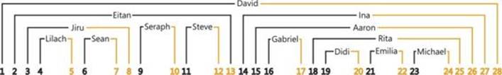
FIGURE 11-10 The nested sets model.

The figure illustrates each employee as spreading two arms around its subordinates. Left and right values can now be assigned to the different arms by simply incrementing a counter from left to right. Keep this illustration in mind—it’s the key to understanding the solution I will present.

Again, the baseline is the original algorithm that traverses a subtree one level at a time and constructs a binary sort path based on a desired ordering of siblings (for example, empname, empid).

Note

For good performance, you should create an index on the parent ID and sort columns—for example, (mgrid, empname, empid).

Instead of generating one row for each node (as was the case in the earlier solutions for generating sort values based on a binary path), you generate two rows by cross-joining each level with an auxiliary table that has two numbers: n=1 represents the left arm, and n=2 represents the right arm. The binary paths are still constructed from row numbers, but in this case the arm number is taken into consideration in addition to the other sort elements (for example, empname, empid, n). The query that returns the next level of subordinates returns the subordinates of the left arm only—again, cross-joined with two numbers (n=1, n=2) to generate two arms for each node.

The following code is the CTE implementation of this algorithm. The purpose of this code is to generate two binary sort paths for each employee that are later used to calculate left and right values. Before you run this code, make sure you have the original Employees table in the tempdb database. If you don’t, rerun the code in Listing 11-1 first:

-- Create index to speed sorting siblings by empname, empid
CREATE UNIQUE INDEX idx_unc_mgrid_empname_empid ON dbo.Employees(mgrid, empname, empid);
GO

DECLARE @root AS INT = 1;

-- CTE with two numbers: 1 and 2
WITH TwoNums AS
(
SELECT n FROM (VALUES(1),(2)) AS D(n)
),
-- CTE with two binary sort paths for each node:
-- One smaller than descendants sort paths
-- One greater than descendants sort paths
SortPath AS
(
SELECT empid, 0 AS lvl, n, CAST(CAST(n AS BINARY(4)) AS VARBINARY(MAX)) AS sort_path
FROM dbo.Employees CROSS JOIN TwoNums
WHERE empid = @root

UNION ALL

SELECT C.empid, P.lvl + 1, TN.n,
P.sort_path + CAST(
( -1 + ROW_NUMBER() OVER(PARTITION BY C.mgrid
-- *** determines order of siblings ***
ORDER BY C.empname, C.empid)) / 2 * 2 + TN.n
AS BINARY(4))
FROM SortPath AS P
INNER JOIN dbo.Employees AS C
ON P.n = 1
AND C.mgrid = P.empid
CROSS JOIN TwoNums AS TN
)
SELECT empid, lvl, n, sort_path FROM SortPath
ORDER BY sort_path;

This code generates the following output:

empid lvl n sort_path
------ ---- -- -------------------------------------------
1 0 1 0x00000001
2 1 1 0x0000000100000001
5 2 1 0x000000010000000100000001
8 3 1 0x00000001000000010000000100000001
8 3 2 0x00000001000000010000000100000002
10 3 1 0x00000001000000010000000100000003
10 3 2 0x00000001000000010000000100000004
5 2 2 0x000000010000000100000002
4 2 1 0x000000010000000100000003
4 2 2 0x000000010000000100000004
6 2 1 0x000000010000000100000005
6 2 2 0x000000010000000100000006
2 1 2 0x0000000100000002
3 1 1 0x0000000100000003
7 2 1 0x000000010000000300000001
11 3 1 0x00000001000000030000000100000001
11 3 2 0x00000001000000030000000100000002
9 3 1 0x00000001000000030000000100000003
14 4 1 0x0000000100000003000000010000000300000001
14 4 2 0x0000000100000003000000010000000300000002
12 4 1 0x0000000100000003000000010000000300000003
12 4 2 0x0000000100000003000000010000000300000004
13 4 1 0x0000000100000003000000010000000300000005
13 4 2 0x0000000100000003000000010000000300000006
9 3 2 0x00000001000000030000000100000004
7 2 2 0x000000010000000300000002
3 1 2 0x0000000100000004
1 0 2 0x00000002

TwoNums is the auxiliary table with two numbers representing the two arms. Of course, if you want to, you can use a real Nums table instead of generating a virtual one.

Two sort paths are generated for each node. The left one is represented by n=1, and the right one is represented by n=2. Notice that for a given node, the left sort path is smaller than all left sort paths of subordinates, and the right sort path is greater than all right sort paths of subordinates. The sort paths are used to generate the left and right values in Figure 11-10. You need to generate left and right integer values to represent the nested sets relationships between the employees. To assign the integer values to the arms (sortval), use the ROW_NUMBER function based onsort_path order. Finally, to return one row for each employee containing the left and right integer values, group the rows by employee and level and return the MIN(sortval) as the left value and MAX(sortval) as the right value. Here’s the complete solution to generate left and right values, followed by its output:

DECLARE @root AS INT = 1;

-- CTE with two numbers: 1 and 2
WITH TwoNums AS
(
SELECT n FROM (VALUES(1),(2)) AS D(n)
),
-- CTE with two binary sort paths for each node:
-- One smaller than descendants sort paths
-- One greater than descendants sort paths
SortPath AS
(
SELECT empid, 0 AS lvl, n, CAST(CAST(n AS BINARY(4)) AS VARBINARY(MAX)) AS sort_path
FROM dbo.Employees CROSS JOIN TwoNums
WHERE empid = @root

UNION ALL

SELECT C.empid, P.lvl + 1, TN.n,
P.sort_path + CAST(
(-1 + ROW_NUMBER() OVER(PARTITION BY C.mgrid
-- *** determines order of siblings ***
ORDER BY C.empname, C.empid)) / 2 * 2 + TN.n
AS BINARY(4))
FROM SortPath AS P
INNER JOIN dbo.Employees AS C
ON P.n = 1
AND C.mgrid = P.empid
CROSS JOIN TwoNums AS TN
),
-- CTE with Row Numbers Representing sort_path Order
Sort AS
(
SELECT empid, lvl, ROW_NUMBER() OVER(ORDER BY sort_path) AS sortval
FROM SortPath
),
-- CTE with Left and Right Values Representing
-- Nested Sets Relationships
NestedSets AS
(
SELECT empid, lvl, MIN(sortval) AS lft, MAX(sortval) AS rgt
FROM Sort
GROUP BY empid, lvl
)
SELECT empid, lvl, lft, rgt FROM NestedSets
ORDER BY lft;

empid lvl lft rgt
------ ---- ---- ----
1 0 1 28
2 1 2 13
5 2 3 8
8 3 4 5
10 3 6 7
4 2 9 10
6 2 11 12
3 1 14 27
7 2 15 26
11 3 16 17
9 3 18 25
14 4 19 20
12 4 21 22
13 4 23 24

Remember the tip I provided earlier concerning the target type of each element in the sort path as a function of the maximum number of children that a single parent can have. I use BINARY(4) in my examples, but remember that you can use a smaller size in some cases.

In the opening paragraph of the “Nested sets” section, I mentioned that this solution is not adequate for large dynamic trees (trees that incur frequent changes). Suppose you stored left and right values in two additional columns in the Employees table. Note that you won’t need the mgridcolumn in the table anymore because the two additional columns with the left and right values are sufficient to answer requests for subordinates, ancestors, and so on. Consider the shake effect of adding a node to the tree. For example, take a look at Figures 11-9 and 11-10 and try to figure out the effect of adding a new subordinate to Steve.

Steve has left and right values of 11 and 12, respectively. The new node should get left and right values of 12 and 13, respectively. Steve’s right value—and in fact all left and right values in the tree that are greater than or equal to 12—should be increased by two. On average, at least half the nodes in the tree must be updated every time a new node is inserted. As you can see here, the shake effect is dramatic. That’s why the nested sets solution is adequate for a large tree only if it’s static or if you need to run queries against a static snapshot of the tree periodically.

Nested sets can provide reasonably good performance with dynamic trees that are small (or forests of small trees)—for example, when maintaining forum discussions where each thread is a small independent tree in a forest. You can implement a solution that synchronizes the left and right values of the tree with every change. You can achieve this by using stored procedures or even triggers, as long as the cost of modification is small enough to be bearable. I won’t even get into variations of the nested sets model that maintain gaps between the values (that is, one that leaves room to insert new leaves without as much work), because they are all ultimately limited.

To generate a table of employees (EmployeesNS) with the employee ID, employee name, salary, level, left values, and right values, join the outer query of the CTE solution and use a SELECT INTO statement. Run the following code to create this as the EmployeesNS table with siblings ordered by empname, empid:

DECLARE @root AS INT = 1;

WITH TwoNums AS
(
SELECT n FROM (VALUES(1),(2)) AS D(n)
),
SortPath AS
(
SELECT empid, 0 AS lvl, n, CAST(CAST(n AS BINARY(4)) AS VARBINARY(MAX)) AS sort_path
FROM dbo.Employees CROSS JOIN TwoNums
WHERE empid = @root

UNION ALL

SELECT C.empid, P.lvl + 1, TN.n,
P.sort_path + CAST(
(-1 + ROW_NUMBER() OVER(PARTITION BY C.mgrid
-- *** determines order of siblings ***
ORDER BY C.empname, C.empid)) / 2 * 2 + TN.n
AS BINARY(4))
FROM SortPath AS P
INNER JOIN dbo.Employees AS C
ON P.n = 1
AND C.mgrid = P.empid
CROSS JOIN TwoNums AS TN
),
Sort AS
(
SELECT empid, lvl, ROW_NUMBER() OVER(ORDER BY sort_path) AS sortval
FROM SortPath
),
NestedSets AS
(
SELECT empid, lvl, MIN(sortval) AS lft, MAX(sortval) AS rgt
FROM Sort
GROUP BY empid, lvl
)
SELECT E.empid, E.empname, E.salary, NS.lvl, NS.lft, NS.rgt
INTO dbo.EmployeesNS
FROM NestedSets AS NS
INNER JOIN dbo.Employees AS E
ON E.empid = NS.empid;

CREATE UNIQUE CLUSTERED INDEX idx_uc_lft ON dbo.EmployeesNS(lft);
ALTER TABLE dbo.EmployeesNS ADD PRIMARY KEY NONCLUSTERED(empid);

In the nested sets model, the left attribute gives you a topological sort order. For this reason, the code creates an index on the lft column.

Querying

The EmployeesNS table models a tree of employees as nested sets. Querying is simple, elegant, and fast for the most part (assuming you have an index on the lft column).

In the following section, I’ll present common requests against a tree and the query solution for each, followed by the output of the query.

Return the subtree of a given root:

The query joins two instances of EmployeesNS. One represents the parent (P) and is filtered by the given root. The other represents the child (C). The two are joined based on the child’s left being between the parent’s left and right values.

Important

You might be tempted to use the predicate C.lft >= P.lft AND C.rgt <= P.rgt because it’s a bit more intuitive than C.lft BETWEEN P.lft AND P.rgt. Both have the same logical meaning in the nested sets model. However, the latter can be optimized much more efficiently in terms of the index access method because it’s based on only one range predicate and not on two like the former.

Indentation of the output is achieved by subtracting the parent level from the child level and replicating the ‘ | ‘ string that number of times. The output is sorted by the child’s left value, which by definition represents topological sorting, and the desired sort of siblings. This subtree query is used as the baseline for most of the following queries.

If you want to exclude the subtree’s root node from the output, simply use greater than (>) and less than (<) operators instead of BETWEEN. To the subtree query, add a filter that returns only nodes where the child’s level minus the parent’s level is smaller than or equal to the requested number of levels under the root.

Return the subtree of a given root, limiting two levels of subordinates under the root:

SELECT C.empid, REPLICATE(' | ', C.lvl - P.lvl) + C.empname AS empname
FROM dbo.EmployeesNS AS P
INNER JOIN dbo.EmployeesNS AS C
ON P.empid = 3
AND C.lft BETWEEN P.lft AND P.rgt
WHERE C.lvl - P.lvl <= 2
ORDER BY C.lft;

empid empname
----------- ---------------
3 Ina
7 | Aaron
11 | | Gabriel
9 | | Rita

Return leaf nodes under a given root:

SELECT C.empid, C.empname
FROM dbo.EmployeesNS AS P
INNER JOIN dbo.EmployeesNS AS C
ON P.empid = 3
AND C.lft BETWEEN P.lft AND P.rgt
WHERE C.rgt - C.lft = 1;

empid empname
----------- ---------
11 Gabriel
14 Didi
12 Emilia
13 Michael

A leaf node is a node for which the right value is greater than the left value by 1 (no subordinates). Add this filter to the subtree query’s WHERE clause. As you can see, the nested sets solution allows for dramatically faster identification of leaf nodes than other solutions that use a NOT EXISTS predicate.

Return the count of subordinates of each node:

Because each node accounts for exactly two lft and rgt values and, in our implementation, no gaps exist, you can calculate the count of subordinates by accessing the subtree’s root alone. The count is (rgt – lft – 1) / 2.

Return all ancestors of a given node:

SELECT P.empid, P.empname, P.lvl
FROM dbo.EmployeesNS AS P
INNER JOIN dbo.EmployeesNS AS C
ON C.empid = 14
AND C.lft BETWEEN P.lft AND P.rgt;

empid empname lvl
------ -------- ----
1 David 0
3 Ina 1
7 Aaron 2
9 Rita 3
14 Didi 4

The ancestors query is almost identical to the subtree query. The nested sets relationships remain the same. The only difference is that here you filter a specific child-node ID, whereas in the subtree query you filtered a specific parent-node ID. Unfortunately, though, from a performance perspective, the path/ancestors query cannot be optimized as well as the subgraph/descendants query because ancestors do not reside in a consecutive range in the index leaf.

When you’re done querying the EmployeesNS table, run the following code for cleanup:

DROP TABLE dbo.EmployeesNS;

Transitive closure

The transitive closure of a directed graph G is the graph with the same nodes as G and with an edge connecting each pair of nodes that are connected by a path (not necessarily containing just one edge) in G. The transitive closure helps answer a number of questions immediately, without the need to explore paths in the graph. For example, is David a manager of Aaron (directly or indirectly)? If the transitive closure of the Employees graph contains an edge from David to Aaron, he is. Does Double Espresso contain water? Can I drive from Los Angeles to New York? If the input graph contains the edges (a, b) and (b, c), a and c have a transitive relationship. The transitive closure contains the edges (a, b), (b, c), and also (a, c). If David is the direct manager of Ina and Ina is the direct manager of Aaron, David transitively is a manager of Aaron, or Aaron transitively is a subordinate of David.

Problems related to transitive closure deal with specialized cases of transitive relationships. An example is the “shortest path” problem, where you’re trying to determine the shortest path between two nodes. For example, what’s the shortest path between Los Angeles and New York?

In this section, I will describe iterative/recursive solutions for transitive closure and shortest-path problems.

Note

The performance of some solutions I will show (specifically those that use recursive CTEs) degrades exponentially as the input graph grows. I’ll present them for demonstration purposes because they are fairly simple and natural. They are adequate for small graphs. Some efficient algorithms for transitive closure–related problems (for example, Floyd’s and Warshall’s algorithms) can be implemented as “level at a time” (breadth-first) iterations. For details on those, refer to http://www.nist.gov/dads/. I’ll show efficient solutions that can be applied to larger graphs.

Directed acyclic graph

The first problem I will discuss is generating a transitive closure of a directed acyclic graph (DAG). Later, I’ll show you how to deal with undirected and cyclic graphs as well. Whether the graph is directed or undirected doesn’t really complicate the solution significantly, but dealing with cyclic graphs does. The input DAG I will use in my example is the BOM I used earlier in the chapter, which you create by running the code in Listing 11-2.

The code that generates the transitive closure of the BOM is somewhat similar to solutions for the subgraph problem (that is, the parts explosion). Specifically, you traverse the graph one level at a time (or, more accurately, you are using breadth-first search techniques). However, instead of returning only a root node here, the anchor member returns all first-level relationships in the BOM. In most graphs, this simply means all existing source/target pairs. In our case, this means all assembly/part pairs where the assembly is not NULL. The recursive member joins the CTE representing the previous level or parent (P) with the BOM representing the next level or child (C). It returns the original product ID (P) as the source and the child product ID (C) as the target. The outer query returns the distinct assembly/part pairs. Keep in mind that multiple paths might lead to a part in the BOM, but you need to return each unique pair only once.

Run the following code to generate the transitive closure of the BOM:

WITH BOMTC AS
(
-- Return all first-level containment relationships
SELECT assemblyid, partid
FROM dbo.BOM
WHERE assemblyid IS NOT NULL

UNION ALL

-- Return next-level containment relationships
SELECT P.assemblyid, C.partid
FROM BOMTC AS P
INNER JOIN dbo.BOM AS C
ON C.assemblyid = P.partid
)
-- Return distinct pairs that have
-- transitive containment relationships
SELECT DISTINCT assemblyid, partid
FROM BOMTC;

This code generates the following output:

assemblyid partid
----------- -----------
1 6
1 7
1 10
1 13
1 14
2 6
2 7
2 10
2 11
2 13
2 14
3 6
3 7
3 11
3 12
3 14
3 16
3 17
4 9
4 12
4 14
4 16
4 17
5 9
5 12
5 14
5 16
5 17
10 13
10 14
12 14
12 16
12 17
16 17

This solution eliminates duplicate edges found in the BOMTC by applying a DISTINCT clause in the outer query. A more efficient solution is to avoid getting duplicates altogether by using a NOT EXISTS predicate in the query that runs repeatedly; such a predicate would filter newly found edges that do not appear in the set of edges that were already found. However, such an implementation can’t use a CTE because the recursive member in the CTE has access only to the immediate previous level, rather than to all previous levels obtained thus far. Instead, you can use a UDF or a stored procedure that invokes the query that runs repeatedly in a loop and inserts each obtained level of nodes into a work table. Run the following code to create the BOMTC UDF, which implements this logic:

IF OBJECT_ID(N'dbo.BOMTC', N'TF') IS NOT NULL DROP FUNCTION dbo.BOMTC;
GO
CREATE FUNCTION BOMTC() RETURNS @BOMTC TABLE
(
assemblyid INT NOT NULL,
partid INT NOT NULL,
PRIMARY KEY (assemblyid, partid)
)
AS
BEGIN
INSERT INTO @BOMTC(assemblyid, partid)
SELECT assemblyid, partid
FROM dbo.BOM
WHERE assemblyid IS NOT NULL

WHILE @@rowcount > 0
INSERT INTO @BOMTC(assemblyid, partid)
SELECT P.assemblyid, C.partid
FROM @BOMTC AS P
INNER JOIN dbo.BOM AS C
ON C.assemblyid = P.partid
WHERE NOT EXISTS
(SELECT * FROM @BOMTC AS P2
WHERE P2.assemblyid = P.assemblyid
AND P2.partid = C.partid);

RETURN;
END
GO

Query the function to get the transitive closure of the BOM:

SELECT assemblyid, partid FROM BOMTC();

If you want to return all paths in the BOM, along with the distance in levels between the parts, you use a similar algorithm with a few additions and revisions. You calculate the distance the same way you calculated the level value in the subgraph/subtree solutions. That is, the anchor assigns a constant distance of 1 for the first level, and the recursive member simply adds one in each iteration. Also, the path calculation is similar to the one used in the subgraph/subtree solutions. The anchor generates a path made of ‘.’ + source_id + ‘.’ + target_id + ‘.’. The recursive member generates it as parent’s path + target_id + ‘.’. Finally, the outer query simply returns all paths (without applying DISTINCT in this case).

Run the following code to generate all possible paths in the BOM and their distances:

WITH BOMPaths AS
(
SELECT assemblyid, partid, 1 AS distance, -- distance in first level is 1
-- path in first level is .assemblyid.partid.
'.' + CAST(assemblyid AS VARCHAR(MAX)) +
'.' + CAST(partid AS VARCHAR(MAX)) + '.' AS path
FROM dbo.BOM
WHERE assemblyid IS NOT NULL

UNION ALL

SELECT P.assemblyid, C.partid,
-- distance in next level is parent's distance + 1
P.distance + 1,
-- path in next level is parent_path.child_partid.
P.path + CAST(C.partid AS VARCHAR(MAX)) + '.'
FROM BOMPaths AS P
INNER JOIN dbo.BOM AS C
ON C.assemblyid = P.partid
)
-- Return all paths
SELECT assemblyid, partid, distance, path
FROM BOMPaths;

You get the following output:

assemblyid partid distance path
----------- ----------- ----------- ----------------
1 6 1 .1.6.
2 6 1 .2.6.
3 6 1 .3.6.
1 7 1 .1.7.
2 7 1 .2.7.
3 7 1 .3.7.
4 9 1 .4.9.
5 9 1 .5.9.
1 10 1 .1.10.
2 10 1 .2.10.
2 11 1 .2.11.
3 11 1 .3.11.
3 12 1 .3.12.
4 12 1 .4.12.
5 12 1 .5.12.
10 13 1 .10.13.
1 14 1 .1.14.
2 14 1 .2.14.
10 14 1 .10.14.
12 14 1 .12.14.
12 16 1 .12.16.
16 17 1 .16.17.
12 17 2 .12.16.17.
5 14 2 .5.12.14.
5 16 2 .5.12.16.
5 17 3 .5.12.16.17.
4 14 2 .4.12.14.
4 16 2 .4.12.16.
4 17 3 .4.12.16.17.
3 14 2 .3.12.14.
3 16 2 .3.12.16.
3 17 3 .3.12.16.17.
2 13 2 .2.10.13.
2 14 2 .2.10.14.
1 13 2 .1.10.13.
1 14 2 .1.10.14.

To isolate only the shortest paths, add a second CTE (BOMRnk) that computes rank values that are partitioned by assembly and part, and ordered by the distance within each partition. In the outer query, filter only the rows with a rank of 1.

Run the following code to produce the shortest paths in the BOM:

WITH BOMPaths AS -- All paths
(
SELECT assemblyid, partid, 1 AS distance,
'.' + CAST(assemblyid AS VARCHAR(MAX)) +
'.' + CAST(partid AS VARCHAR(MAX)) + '.' AS path
FROM dbo.BOM
WHERE assemblyid IS NOT NULL

UNION ALL

SELECT P.assemblyid, C.partid, P.distance + 1,
P.path + CAST(C.partid AS VARCHAR(MAX)) + '.'
FROM BOMPaths AS P
INNER JOIN dbo.BOM AS C
ON C.assemblyid = P.partid
),
BOMRnk AS -- Rank paths
(
SELECT *, RANK() OVER(PARTITION BY assemblyid, partid ORDER BY distance) AS rnk
FROM BOMPaths
)
-- Shortest path for each pair
SELECT assemblyid, partid, distance, path
FROM BOMRnk
WHERE rnk = 1;

This code generates the following output:

assemblyid partid distance path
----------- ----------- ----------- ------------------
1 6 1 .1.6.
1 7 1 .1.7.
1 10 1 .1.10.
1 13 2 .1.10.13.
1 14 1 .1.14.
2 6 1 .2.6.
2 7 1 .2.7.
2 10 1 .2.10.
2 11 1 .2.11.
2 13 2 .2.10.13.
2 14 1 .2.14.
3 6 1 .3.6.
3 7 1 .3.7.
3 11 1 .3.11.
3 12 1 .3.12.
3 14 2 .3.12.14.
3 16 2 .3.12.16.
3 17 3 .3.12.16.17.
4 9 1 .4.9.
4 12 1 .4.12.
4 14 2 .4.12.14.
4 16 2 .4.12.16.
4 17 3 .4.12.16.17.
5 9 1 .5.9.
5 12 1 .5.12.
5 14 2 .5.12.14.
5 16 2 .5.12.16.
5 17 3 .5.12.16.17.
10 13 1 .10.13.
10 14 1 .10.14.
12 14 1 .12.14.
12 16 1 .12.16.
12 17 2 .12.16.17.
16 17 1 .16.17.

Undirected cyclic graph

Even though transitive closure is defined for a directed graph, you can also define and generate it for undirected graphs where each edge represents a two-way relationship. In my examples, I will use the Roads graph, which you create and populate by running the code in Listing 11-3. To see a visual representation of Roads, examine Figure 11-4. To apply the transitive-closure and shortest-path solutions to Roads, first convert it to a digraph by generating two directed edges from each existing edge:

SELECT city1 AS from_city, city2 AS to_city FROM dbo.Roads
UNION ALL
SELECT city2, city1 FROM dbo.Roads

For example, the edge (JFK, ATL) in the undirected graph appears as two edges, (JFK, ATL) and (ATL, JFK), in the digraph. The former represents the road from New York to Atlanta, and the latter represents the road from Atlanta to New York.

Because Roads is a cyclic graph, you also need to use the cycle-detection logic I described earlier in the chapter to avoid traversing cyclic paths. Armed with the techniques to generate a digraph out of an undirected graph and to detect cycles, you have all the tools you need to produce the transitive closure of Roads.

Run the following code to generate the transitive closure of Roads:

WITH Roads2 AS -- Two rows for each pair (from-->to, to-->from)
(
SELECT city1 AS from_city, city2 AS to_city FROM dbo.Roads
UNION ALL
SELECT city2, city1 FROM dbo.Roads
),
RoadPaths AS
(
-- Return all first-level reachability pairs
SELECT from_city, to_city,
-- path is needed to identify cycles
CAST('.' + from_city + '.' + to_city + '.' AS VARCHAR(MAX)) AS path
FROM Roads2

UNION ALL

-- Return next-level reachability pairs
SELECT F.from_city, T.to_city, CAST(F.path + T.to_city + '.' AS VARCHAR(MAX))
FROM RoadPaths AS F
INNER JOIN Roads2 AS T
-- if to_city appears in from_city's path, cycle detected
ON CASE WHEN F.path LIKE '%.' + T.to_city + '.%'
THEN 1 ELSE 0 END = 0
AND F.to_city = T.from_city
)
-- Return Transitive Closure of Roads
SELECT DISTINCT from_city, to_city
FROM RoadPaths;

The Roads2 CTE creates the digraph out of Roads. The RoadPaths CTE returns all possible source/target pairs (and has a big performance penalty), and it avoids returning and pursuing a path for which a cycle is detected. The outer query returns all distinct source/target pairs, shown next.

from to from to from to from to from to
---- ---- ---- ---- ---- ---- ---- ---- ---- ----
ANC FAI IAH LAX LAX SEA MSP JFK SEA ORD
ATL DEN IAH MCI LAX SFO MSP LAX SEA SFO
ATL IAH IAH MIA MCI ATL MSP MCI SFO ATL
ATL JFK IAH MSP MCI DEN MSP MIA SFO DEN
ATL LAX IAH ORD MCI IAH MSP ORD SFO IAH
ATL MCI IAH SEA MCI JFK MSP SEA SFO JFK
ATL MIA IAH SFO MCI LAX MSP SFO SFO LAX
ATL MSP JFK ATL MCI MIA ORD ATL SFO MCI
ATL ORD JFK DEN MCI MSP ORD DEN SFO MIA
ATL SEA JFK IAH MCI ORD ORD IAH SFO MSP
ATL SFO JFK LAX MCI SEA ORD JFK SFO ORD
DEN ATL JFK MCI MCI SFO ORD LAX SFO SEA
DEN IAH JFK MIA MIA ATL ORD MCI
DEN JFK JFK MSP MIA DEN ORD MIA
DEN LAX JFK ORD MIA IAH ORD MSP
DEN MCI JFK SEA MIA JFK ORD SEA
DEN MIA JFK SFO MIA LAX ORD SFO
DEN MSP LAX ATL MIA MCI SEA ATL
DEN ORD LAX DEN MIA MSP SEA DEN
DEN SEA LAX IAH MIA ORD SEA IAH
DEN SFO LAX JFK MIA SEA SEA JFK
FAI ANC LAX MCI MIA SFO SEA LAX
IAH ATL LAX MIA MSP ATL SEA MCI
IAH DEN LAX MSP MSP DEN SEA MIA
IAH JFK LAX ORD MSP IAH SEA MSP

Here, as well, you can use loops instead of a recursive CTE to optimize the solution, as demonstrated earlier with the BOM scenario. Run the following code to create the RoadsTC UDF, which returns the transitive closure of Roads using loops:

IF OBJECT_ID(N'dbo.RoadsTC', N'TF') IS NOT NULL DROP FUNCTION dbo.RoadsTC;
GO
CREATE FUNCTION dbo.RoadsTC() RETURNS @RoadsTC TABLE
(
from_city VARCHAR(3) NOT NULL,
to_city VARCHAR(3) NOT NULL,
PRIMARY KEY (from_city, to_city)
)
AS
BEGIN
DECLARE @added as INT;

INSERT INTO @RoadsTC(from_city, to_city)
SELECT city1, city2 FROM dbo.Roads;

SET @added = @@rowcount;

INSERT INTO @RoadsTC
SELECT city2, city1 FROM dbo.Roads

SET @added = @added + @@rowcount;

WHILE @added > 0 BEGIN

INSERT INTO @RoadsTC
SELECT DISTINCT TC.from_city, R.city2
FROM @RoadsTC AS TC
INNER JOIN dbo.Roads AS R
ON R.city1 = TC.to_city
WHERE NOT EXISTS
(SELECT * FROM @RoadsTC AS TC2
WHERE TC2.from_city = TC.from_city
AND TC2.to_city = R.city2)
AND TC.from_city <> R.city2;

SET @added = @@rowcount;

INSERT INTO @RoadsTC
SELECT DISTINCT TC.from_city, R.city1
FROM @RoadsTC AS TC
INNER JOIN dbo.Roads AS R
ON R.city2 = TC.to_city
WHERE NOT EXISTS
(SELECT * FROM @RoadsTC AS TC2
WHERE TC2.from_city = TC.from_city
AND TC2.to_city = R.city1)
AND TC.from_city <> R.city1;

SET @added = @added + @@rowcount;
END
RETURN;
END
GO

-- Use the RoadsTC UDF
SELECT from_city, to_city FROM dbo.RoadsTC();
GO

Run the following query to get the transitive closure of Roads:

SELECT from_city, to_city FROM dbo.RoadsTC();

To return all paths and distances, use similar logic to the one used in the digraph solution in the previous section. The difference here is that the distance is not just a level counter—it is the sum of the distances along the route from one city to the other.

Run the following code to return all paths and distances in Roads:

WITH Roads2 AS
(
SELECT city1 AS from_city, city2 AS to_city, distance FROM dbo.Roads
UNION ALL
SELECT city2, city1, distance FROM dbo.Roads
),
RoadPaths AS
(
SELECT from_city, to_city, distance,
CAST('.' + from_city + '.' + to_city + '.' AS VARCHAR(MAX)) AS path
FROM Roads2

UNION ALL

SELECT F.from_city, T.to_city, F.distance + T.distance,
CAST(F.path + T.to_city + '.' AS VARCHAR(MAX))
FROM RoadPaths AS F
INNER JOIN Roads2 AS T
ON CASE WHEN F.path LIKE '%.' + T.to_city + '.%'
THEN 1 ELSE 0 END = 0
AND F.to_city = T.from_city
)
-- Return all paths and distances
SELECT from_city, to_city, distance, path
FROM RoadPaths;

Finally, to return shortest paths in Roads, use the same logic as the digraph shortest-paths solution. Run the following code to return shortest paths in Roads:

WITH Roads2 AS
(
SELECT city1 AS from_city, city2 AS to_city, distance FROM dbo.Roads
UNION ALL
SELECT city2, city1, distance FROM dbo.Roads
),
RoadPaths AS
(
SELECT from_city, to_city, distance,
CAST('.' + from_city + '.' + to_city + '.' AS VARCHAR(MAX)) AS path
FROM Roads2

UNION ALL

SELECT F.from_city, T.to_city, F.distance + T.distance,
CAST(F.path + T.to_city + '.' AS VARCHAR(MAX))
FROM RoadPaths AS F
INNER JOIN Roads2 AS T
ON CASE WHEN F.path LIKE '%.' + T.to_city + '.%'
THEN 1 ELSE 0 END = 0
AND F.to_city = T.from_city
),
RoadsRnk AS -- Rank paths
(
SELECT *, RANK() OVER(PARTITION BY from_city, to_city ORDER BY distance) AS rnk
FROM RoadPaths
)
-- Return shortest paths and distances
SELECT from_city, to_city, distance, path
FROM RoadsRnk
WHERE rnk = 1;

You get the following output:

from_city to_city distance path
--------- ------- ----------- ------------------------
ANC FAI 359 .ANC.FAI.
ATL IAH 800 .ATL.IAH.
ATL JFK 865 .ATL.JFK.
ATL MCI 805 .ATL.MCI.
ATL MIA 665 .ATL.MIA.
ATL ORD 715 .ATL.ORD.
DEN IAH 1120 .DEN.IAH.
DEN LAX 1025 .DEN.LAX.
DEN MCI 600 .DEN.MCI.
DEN MSP 915 .DEN.MSP.
DEN SEA 1335 .DEN.SEA.
DEN SFO 1270 .DEN.SFO.
IAH LAX 1550 .IAH.LAX.
IAH MCI 795 .IAH.MCI.
IAH MIA 1190 .IAH.MIA.
JFK ORD 795 .JFK.ORD.
LAX SFO 385 .LAX.SFO.
MCI MSP 440 .MCI.MSP.
MCI ORD 525 .MCI.ORD.
MSP ORD 410 .MSP.ORD.
MSP SEA 2015 .MSP.SEA.
SEA SFO 815 .SEA.SFO.
FAI ANC 359 .FAI.ANC.
IAH ATL 800 .IAH.ATL.
JFK ATL 865 .JFK.ATL.
MCI ATL 805 .MCI.ATL.
MIA ATL 665 .MIA.ATL.
ORD ATL 715 .ORD.ATL.
IAH DEN 1120 .IAH.DEN.
LAX DEN 1025 .LAX.DEN.
MCI DEN 600 .MCI.DEN.
MSP DEN 915 .MSP.DEN.
SEA DEN 1335 .SEA.DEN.
SFO DEN 1270 .SFO.DEN.
LAX IAH 1550 .LAX.IAH.
MCI IAH 795 .MCI.IAH.
MIA IAH 1190 .MIA.IAH.
ORD JFK 795 .ORD.JFK.
SFO LAX 385 .SFO.LAX.
MSP MCI 440 .MSP.MCI.
ORD MCI 525 .ORD.MCI.
ORD MSP 410 .ORD.MSP.
SEA MSP 2015 .SEA.MSP.
SFO SEA 815 .SFO.SEA.
SEA ORD 2425 .SEA.MSP.ORD.
SEA JFK 3220 .SEA.MSP.ORD.JFK.
ORD SEA 2425 .ORD.MSP.SEA.
ORD DEN 1125 .ORD.MCI.DEN.
ORD IAH 1320 .ORD.MCI.IAH.
ORD LAX 2150 .ORD.MCI.DEN.LAX.
ORD SFO 2395 .ORD.MCI.DEN.SFO.
MSP IAH 1235 .MSP.MCI.IAH.
SFO IAH 1935 .SFO.LAX.IAH.
SFO MIA 3125 .SFO.LAX.IAH.MIA.
MIA LAX 2740 .MIA.IAH.LAX.
MIA SFO 3125 .MIA.IAH.LAX.SFO.
LAX MIA 2740 .LAX.IAH.MIA.
LAX ATL 2350 .LAX.IAH.ATL.
SFO MCI 1870 .SFO.DEN.MCI.
SFO MSP 2185 .SFO.DEN.MSP.
SFO ORD 2395 .SFO.DEN.MCI.ORD.
SFO ATL 2675 .SFO.DEN.MCI.ATL.
SFO JFK 3190 .SFO.DEN.MCI.ORD.JFK.
SEA IAH 2455 .SEA.DEN.IAH.
SEA MCI 1935 .SEA.DEN.MCI.
SEA ATL 2740 .SEA.DEN.MCI.ATL.
SEA MIA 3405 .SEA.DEN.MCI.ATL.MIA.
MSP LAX 1940 .MSP.DEN.LAX.
MSP SFO 2185 .MSP.DEN.SFO.
MCI LAX 1625 .MCI.DEN.LAX.
MCI SEA 1935 .MCI.DEN.SEA.
MCI SFO 1870 .MCI.DEN.SFO.
LAX MCI 1625 .LAX.DEN.MCI.
LAX MSP 1940 .LAX.DEN.MSP.
LAX ORD 2150 .LAX.DEN.MCI.ORD.
LAX JFK 2945 .LAX.DEN.MCI.ORD.JFK.
IAH SEA 2455 .IAH.DEN.SEA.
ORD MIA 1380 .ORD.ATL.MIA.
MIA JFK 1530 .MIA.ATL.JFK.
MIA MCI 1470 .MIA.ATL.MCI.
MIA ORD 1380 .MIA.ATL.ORD.
MIA MSP 1790 .MIA.ATL.ORD.MSP.
MIA DEN 2070 .MIA.ATL.MCI.DEN.
MIA SEA 3405 .MIA.ATL.MCI.DEN.SEA.
MCI MIA 1470 .MCI.ATL.MIA.
JFK IAH 1665 .JFK.ATL.IAH.
JFK MIA 1530 .JFK.ATL.MIA.
IAH JFK 1665 .IAH.ATL.JFK.
SEA LAX 1200 .SEA.SFO.LAX.
MSP ATL 1125 .MSP.ORD.ATL.
MSP JFK 1205 .MSP.ORD.JFK.
MSP MIA 1790 .MSP.ORD.ATL.MIA.
MCI JFK 1320 .MCI.ORD.JFK.
LAX SEA 1200 .LAX.SFO.SEA.
JFK MCI 1320 .JFK.ORD.MCI.
JFK MSP 1205 .JFK.ORD.MSP.
JFK SEA 3220 .JFK.ORD.MSP.SEA.
JFK DEN 1920 .JFK.ORD.MCI.DEN.
JFK LAX 2945 .JFK.ORD.MCI.DEN.LAX.
JFK SFO 3190 .JFK.ORD.MCI.DEN.SFO.
IAH MSP 1235 .IAH.MCI.MSP.
IAH ORD 1320 .IAH.MCI.ORD.
IAH SFO 1935 .IAH.LAX.SFO.
DEN ORD 1125 .DEN.MCI.ORD.
DEN ATL 1405 .DEN.MCI.ATL.
DEN MIA 2070 .DEN.MCI.ATL.MIA.
DEN JFK 1920 .DEN.MCI.ORD.JFK.
ATL MSP 1125 .ATL.ORD.MSP.
ATL DEN 1405 .ATL.MCI.DEN.
ATL SEA 2740 .ATL.MCI.DEN.SEA.
ATL SFO 2675 .ATL.MCI.DEN.SFO.
ATL LAX 2350 .ATL.IAH.LAX.

To satisfy multiple requests for the shortest paths between two cities, you might want to materialize the result set in a table and index it, like so:

WITH Roads2 AS
(
SELECT city1 AS from_city, city2 AS to_city, distance FROM dbo.Roads
UNION ALL
SELECT city2, city1, distance FROM dbo.Roads
),
RoadPaths AS
(
SELECT from_city, to_city, distance,
CAST('.' + from_city + '.' + to_city + '.' AS VARCHAR(MAX)) AS path
FROM Roads2

UNION ALL

SELECT F.from_city, T.to_city, F.distance + T.distance,
CAST(F.path + T.to_city + '.' AS VARCHAR(MAX))
FROM RoadPaths AS F
INNER JOIN Roads2 AS T
ON CASE WHEN F.path LIKE '%.' + T.to_city + '.%'
THEN 1 ELSE 0 END = 0
AND F.to_city = T.from_city
),
RoadsRnk AS -- Rank paths
(
SELECT *, RANK() OVER(PARTITION BY from_city, to_city ORDER BY distance) AS rnk
FROM RoadPaths
)
-- Return shortest paths and distances
SELECT from_city, to_city, distance, path
INTO dbo.RoadPaths
FROM RoadsRnk
WHERE rnk = 1;

CREATE UNIQUE CLUSTERED INDEX idx_uc_from_city_to_city
ON dbo.RoadPaths(from_city, to_city);

Once the result set is materialized and indexed, a request for the shortest path between two cities can be satisfied instantly. This is practical and advisable when information changes infrequently. As is often the case, there is a trade-off between up to date and fast. The following query requests the shortest path between Los Angeles and New York:

SELECT from_city, to_city, distance, path FROM dbo.RoadPaths
WHERE from_city = 'LAX' AND to_city = 'JFK';

This query generates the following output:

from_city to_city distance path
--------- ------- ----------- ----------------------
LAX JFK 2945 .LAX.DEN.MCI.ORD.JFK.

A more efficient solution to the shortest-paths problem uses loops instead of recursive CTEs. It is more efficient for reasons similar to the ones described earlier; that is, in each iteration of the loop you have access to all previously spooled data and not just to the immediate previous level. You create a function called RoadsTC that returns a table variable called @RoadsTC. The table variable has the attributes from_city, to_city, distance, and route, which are self-explanatory. The function’s code first inserts into @RoadsTC a row for each (city1, city2) and (city2, city1) pair from the table Roads. The code then enters a loop that iterates as long as the previous iteration inserted rows to @RoadsTC. In each iteration of the loop, the code inserts new routes that extend the existing routes in @RoadsTC. New routes are added only if the source and destination do not appear already in @RoadsTC with the same distance or a shorter distance. Run the following code to create the RoadsTC function.

IF OBJECT_ID(N'dbo.RoadsTC', N'TF') IS NOT NULL DROP FUNCTION dbo.RoadsTC;
GO
CREATE FUNCTION dbo.RoadsTC() RETURNS @RoadsTC TABLE
(
uniquifier INT NOT NULL IDENTITY,
from_city VARCHAR(3) NOT NULL,
to_city VARCHAR(3) NOT NULL,
distance INT NOT NULL,
route VARCHAR(MAX) NOT NULL,
PRIMARY KEY (from_city, to_city, uniquifier)
)
AS
BEGIN
DECLARE @added AS INT;

INSERT INTO @RoadsTC
SELECT city1 AS from_city, city2 AS to_city, distance, '.' + city1 + '.' + city2 + '.'
FROM dbo.Roads;

SET @added = @@rowcount;

INSERT INTO @RoadsTC
SELECT city2, city1, distance, '.' + city2 + '.' + city1 + '.'
FROM dbo.Roads;

SET @added = @added + @@rowcount;

WHILE @added > 0 BEGIN
INSERT INTO @RoadsTC
SELECT DISTINCT TC.from_city, R.city2, TC.distance + R.distance, TC.route + city2 + '.'
FROM @RoadsTC AS TC
INNER JOIN dbo.Roads AS R
ON R.city1 = TC.to_city
WHERE NOT EXISTS
(SELECT * FROM @RoadsTC AS TC2
WHERE TC2.from_city = TC.from_city
AND TC2.to_city = R.city2
AND TC2.distance <= TC.distance + R.distance)
AND TC.from_city <> R.city2;

SET @added = @@rowcount;

INSERT INTO @RoadsTC
SELECT DISTINCT TC.from_city, R.city1, TC.distance + R.distance, TC.route + city1 + '.'
FROM @RoadsTC AS TC
INNER JOIN dbo.Roads AS R
ON R.city2 = TC.to_city
WHERE NOT EXISTS
(SELECT * FROM @RoadsTC AS TC2
WHERE TC2.from_city = TC.from_city
AND TC2.to_city = R.city1
AND TC2.distance <= TC.distance + R.distance)
AND TC.from_city <> R.city1;

SET @added = @added + @@rowcount;
END
RETURN;
END
GO

The function might return more than one row for the same source and target cities. To return shortest paths and distances, use the following query:

SELECT from_city, to_city, distance, route
FROM (SELECT from_city, to_city, distance, route,
RANK() OVER (PARTITION BY from_city, to_city ORDER BY distance) AS rnk
FROM dbo.RoadsTC() AS F) AS RTC
WHERE rnk = 1;

This solution applies logic similar to the CTE-based solution to filter the shortest paths. The derived table query assigns a rank value (rnk) to each row, based on from_city, to_city partitioning and distance ordering. This means that shortest paths are assigned with the rank value 1. The outer query filters only the shortest paths (rnk = 1).

When you’re done querying the RoadPaths table, don’t forget to drop it:

DROP TABLE dbo.RoadPaths;

Conclusion

This chapter covered the treatment of graphs. I presented iterative/recursive solutions as well as ones that materialize extra information about the relationships in the graph.

The main advantage of the iterative/recursive solutions is that you don’t need to materialize and maintain any additional attributes—the graph manipulation is based on the stored edge attributes. The materialized path solution materializes an enumerated path and possibly also the level for each node and path that leads to it. You can either maintain your own custom materialized path or use SQL Server’s proprietary HIERARCHYID data type.

In the materialized path solution, the maintenance of the additional information is not very expensive, and you benefit from simple and fast set-based queries. The nested sets solution materializes left and right values representing set containment relationships and possibly the level as well. This is probably the most elegant solution of those I presented, and it also allows for simple and fast queries. However, maintaining the materialized information is expensive, so typically this solution is practical for either static trees or small dynamic trees.

In the last section, I presented solutions to transitive-closure and shortest-path problems.

Because this chapter concludes the book, I’d like to leave you with a final thought. If you ask me what the most important thing is that I hope you get from this book, I’d say it is the importance of paying special attention to fundamentals. Do not underestimate them or take them lightly. Spend time on identifying, focusing on, and perfecting fundamental techniques. When you are faced with a tough problem, solutions will flow naturally.

“Matters of great concern should be treated lightly.”

“Matters of small concern should be treated seriously.”

—Hagakure, The Book of the Samurai by Yamamoto Tsunetomo

The meaning of these sayings is not what appears on the surface. The book goes on to explain:

“Among one’s affairs there should not be more than two or three matters of what one could call great concern. If these are deliberated upon during ordinary times, they can be understood. Thinking about things previously and then handling them lightly when the time comes is what this is all about. To face an event and solve it lightly is difficult if you are not resolved beforehand, and there will always be uncertainty in hitting your mark. However, if the foundation is laid previously, you can think of the saying, ‘Matters of great concern should be treated lightly,’ as your own basis for action.”