CCNA Wireless 200-355 Official Cert Guide (2016)
Chapter 1. RF Signals and Modulation
This chapter covers the following topics:
![]() Comparing Wired and Wireless Networks—This section provides a brief overview of how a wireless network differs from a wired network.
Comparing Wired and Wireless Networks—This section provides a brief overview of how a wireless network differs from a wired network.
![]() Understanding Basic Wireless Theory—This section discusses radio frequency signals and their properties, such as frequency, bandwidth, phase, wavelength, and power level.
Understanding Basic Wireless Theory—This section discusses radio frequency signals and their properties, such as frequency, bandwidth, phase, wavelength, and power level.
![]() Carrying Data over an RF Signal—This section covers the encoding and modulation methods that are used in wireless LANs.
Carrying Data over an RF Signal—This section covers the encoding and modulation methods that are used in wireless LANs.
This chapter covers the following exam topics:
![]() 1.1—Describe the propagation of radio waves
1.1—Describe the propagation of radio waves
![]() 1.1a—Frequency, amplitude, phase, wavelength (characteristics)
1.1a—Frequency, amplitude, phase, wavelength (characteristics)
![]() 1.2—Interpret RF signal measurements
1.2—Interpret RF signal measurements
![]() 1.2a—Signal strength (RSSI, transmit power, receive sensitivity)
1.2a—Signal strength (RSSI, transmit power, receive sensitivity)
![]() 1.2b—Differentiate interference vs. noise
1.2b—Differentiate interference vs. noise
![]() 1.2d—Define SNR
1.2d—Define SNR
![]() 1.3—Explain the principles of RF mathematics
1.3—Explain the principles of RF mathematics
![]() 1.3a—Compute dBm, mW, Law of 3s and 10s
1.3a—Compute dBm, mW, Law of 3s and 10s
![]() 1.4—Describe Wi-Fi antenna characteristics
1.4—Describe Wi-Fi antenna characteristics
![]() 1.4c—dBi, dBd, EIRP
1.4c—dBi, dBd, EIRP
![]() 2.3—Describe 802.11 fundamentals
2.3—Describe 802.11 fundamentals
![]() 2.3a—Modulation techniques
2.3a—Modulation techniques
Wireless LANs must transmit a signal over radio frequencies (RF) to move data from one device to another. Transmitters and receivers can be fixed in consistent locations or they can be free to move around. This chapter covers the basic theory behind RF signals and the methods used to carry data wirelessly.
“Do I Know This Already?” Quiz
The “Do I Know This Already?” quiz allows you to assess whether you should read this entire chapter thoroughly or jump to the “Exam Preparation Tasks” section. If you are in doubt about your answers to these questions or your own assessment of your knowledge of the topics, read the entire chapter. Table 1-1 lists the major headings in this chapter and their corresponding “Do I Know This Already?” quiz questions. You can find the answers in Appendix A, “Answers to the ‘Do I Know This Already?’ Quizzes.”
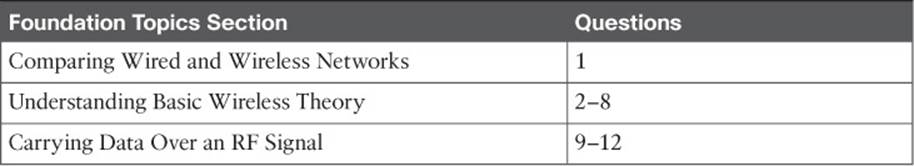
Table 1-1 “Do I Know This Already?” Section-to-Question Mapping
Caution
The goal of self-assessment is to gauge your mastery of the topics in this chapter. If you do not know the answer to a question or are only partially sure of the answer, you should mark that question as wrong for purposes of the self-assessment. Giving yourself credit for an answer you correctly guess skews your self-assessment results and might provide you with a false sense of security.
1. Which one of the following is the common standard that defines wireless LAN operation?
a. IEEE 802.1
b. IEEE 802.1x
c. IEEE 802.11
d. IEEE 802.3
2. Which of the following represent the frequency bands commonly used for wireless LANs? (Choose two.)
a. 2.4 MHz
b. 2.4 GHz
c. 5.5 MHz
d. 11 GHz
e. 5 GHz
3. Two transmitters are each operating with a transmit power level of 100 mW. When you compare the two absolute power levels, what is the difference in dB?
a. 0 dB
b. 20 dB
c. 100 dB
d. You can’t compare power levels in dB.
4. A transmitter is configured to use a power level of 17 mW. One day it is reconfigured to transmit at a new power level of 34 mW. How much has the power level increased in dB?
a. 0 dB
b. 2 dB
c. 3 dB
d. 17 dB
e. None of these answers are correct; you need a calculator to figure this out.
5. Transmitter A has a power level of 1 mW, and transmitter B is 100 mW. Compare transmitter B to A using dB, and then identify the correct answer from the following choices.
a. 0 dB
b. 1 dB
c. 10 dB
d. 20 dB
e. 100 dB
6. A transmitter normally uses an absolute power level of 100 mW. Through the course of needed changes, its power level is reduced to 40 mW. What is the power-level change in dB?
a. 2.5 dB
b. 4 dB
c. –4 dB
d. –40 dB
e. None of these answers are correct; where is that calculator?
7. Consider a scenario with a transmitter and a receiver that are separated by some distance. The transmitter uses an absolute power level of 20 dBm. A cable connects the transmitter to its antenna. The receiver also has a cable connecting it to its antenna. Each cable has a loss of 2 dB. The transmitting and receiving antennas each have a gain of 5 dBi. What is the resulting EIRP?
a. +20 dBm
b. +23 dBm
c. +26 dBm
d. +34 dBm
e. None of these answers are correct.
8. A receiver picks up an RF signal from a distant transmitter. Which one of the following represents the best signal quality received? Example values are given in parentheses.
a. Low SNR (10 dB), Low RSSI (–75)
b. High SNR (30 dB), Low RSSI (–75)
c. Low SNR (10 dB), High RSSI (–30)
d. High SNR (30 dB), High RSSI (–30)
9. The typical data rates of 1, 2, 5.5, and 11 Mbps can be supported by which one of the following modulation types?
a. OFDM
b. FHSS
c. DSSS
d. QAM
10. Put the following modulation schemes in order of the number of possible changes that can be made to the carrier signal, from lowest to highest.
a. 16-QAM
b. DQPSK
c. DBPSK
d. 64-QAM
11. 64-QAM modulation alters which two of the following aspects of an RF signal?
a. Frequency
b. Amplitude
c. Phase
d. Quadrature
12. OFDM offers data rates up to 54 Mbps, but DSSS supports much lower limits. Compared with DSSS, which one of the following does OFDM leverage to achieve its superior data rates?
a. Higher-frequency band
b. Wider 20-MHz channel width
c. 48 subcarriers in a channel
d. Faster chipping rates
e. Greater number of channels in a band
Foundation Topics
Comparing Wired and Wireless Networks
In a wired network, any two devices that need to communicate with each other must be connected by a wire. (That was obvious!) The “wire” might contain strands of metal or fiber-optic material that run continuously from one end to the other. Data that passes over the wire is bounded by the physical properties of the wire. In fact, the IEEE 802.3 set of standards defines strict guidelines for the Ethernet wire itself, in addition to how devices may connect, send, and receive data over the wire.
Wired connections have been engineered with tight constraints and have few variables that might prevent successful communication. Even the type and size of the wire strands, the number of twists the strands must make around each other over a distance, and the maximum length of the wire must adhere to the standard.
Therefore, a wired network is essentially a bounded medium; data must travel over whatever path the wire or cable takes between two devices. If the cable goes around a corner or lies in a coil, the electrical signals used to carry the data must also go around a corner or around a coil. Because only two devices may connect to a wire, only those two devices may send or transmit data. Even better: The two devices may transmit data to each other simultaneously because they each have a private, direct path to each other.
Wired networks also have some shortcomings. When a device is connected by a wire, it cannot move around very easily or very far. Before a device can connect to a wired network, it must have a connector that is compatible with the one on the end of the wire. As devices get smaller and more mobile, it just is not practical to connect them to a wire.
As its name implies, a wireless network removes the need to be tethered to a wire or cable. Convenience and mobility become paramount, enabling users to move around at will while staying connected to the network. A user can (and often does) bring along many different wireless devices that can all connect to the network easily and seamlessly.
Wireless data must travel through free space, without the constraints and protection of a wire. In the free space environment, many variables can affect the data and its delivery. To minimize the variables, wireless engineering efforts must focus on two things:
![]() Wireless devices must adhere to a common standard.
Wireless devices must adhere to a common standard.
![]() Wireless coverage must exist in the area where devices are expected.
Wireless coverage must exist in the area where devices are expected.
Wireless LANs are based on the IEEE 802.11 standard, which is covered in more detail in Chapter 2, “RF Standards.”
Understanding Basic Wireless Theory
To send data across a wired link, an electrical signal is applied at one end and is carried to the other end. The wire itself is continuous and conductive, so the signal can propagate rather easily. A wireless link has no physical strands of anything to carry the signal along.
How then can an electrical signal be sent across the air, or free space? Consider a simple analogy of two people standing far apart, and one person wants to signal something to other. They are connected by a long and somewhat-loose rope; the rope represents free space. The sender at one end decides to lift his end of the rope high and hold it there so that the other end of the rope will also raise and notify the partner. After all, if the rope were a wire, he knows that he could apply a steady voltage at one end of the wire and it would appear at the other end. Figure 1-1 shows the end result; the rope falls back down after a tiny distance, and the receiver never notices a change.
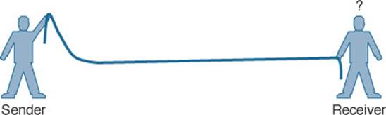
Figure 1-1 Failed Attempt to Pass a Message Down a Rope
The sender tries a different strategy. He cannot push the rope, but when he begins to wave it up and down in a steady, regular motion, a curious thing happens. A continuous wave pattern appears along the entire length of the rope, as shown in Figure 1-2. In fact, the waves (each representing one up and down cycle of the sender’s arm) actually travel from the sender to the receiver.
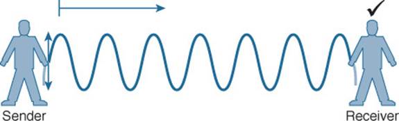
Figure 1-2 Sending a Continuous Wave Down a Rope
In free space, a similar principle occurs. The sender (a transmitter) can send an alternating current into a section of wire (an antenna), which sets up moving electric and magnetic fields that propagate out and away as traveling waves. The electric and magnetic fields travel along together and are always at right angles to each other, as shown in Figure 1-3. The signal must keep changing, or alternating, by cycling up and down, to keep the electric and magnetic fields cycling and pushing ever outward.
Figure 1-3 Traveling Electric and Magnetic Waves
Electromagnetic waves do not travel in a straight line. Instead, they travel by expanding in all directions away from the antenna. To get a visual image, think of dropping a pebble into a pond when the surface is still. Where it drops in, the pebble sets the water’s surface into a cyclic motion. The waves that result begin small and expand outward, only to be replaced by new waves. In free space, the electromagnetic waves expand outward in all three dimensions.
Figure 1-4 shows a simple idealistic antenna that is a single point at the end of a wire. The waves produced expand outward in a spherical shape. The waves will eventually reach the receiver, in addition to many other locations in other directions.
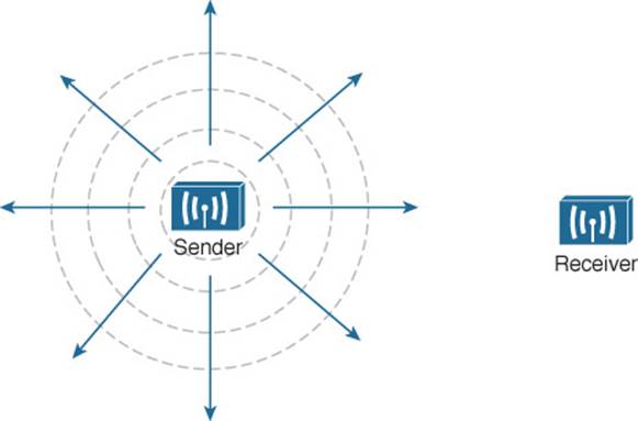
Figure 1-4 Wave Propagation with an Idealistic Antenna
Tip
The idealistic antenna does not really exist, but serves as a reference point to understand wave propagation. In the real world, antennas can be made in various shapes and forms that can limit the direction that the waves are sent. Chapter 4, “Understanding Antennas,” covers antennas in more detail.
At the receiving end of a wireless link, the process is reversed. As the electromagnetic waves reach the receiver’s antenna, they induce an electrical signal. If everything works right, the received signal will be a reasonable copy of the original transmitted signal.
Understanding Frequency
The waves involved in a wireless link can be measured and described in several ways. One fundamental property is the frequency of the wave, or the number of times the signal makes one complete up and down cycle in 1 second. Figure 1-5 shows how a cycle of a wave can be identified. A cycle can begin as the signal rises from the center line, falls through the center line, and rises again to meet the center line. A cycle can also be measured from the center of one peak to the center of the next peak. No matter where you start measuring a cycle, the signal must make a complete sequence back to its starting position where it is ready to repeat the same cyclic pattern again.
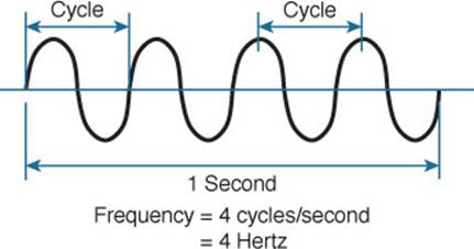
Figure 1-5 Cycles Within a Wave
In Figure 1-5, suppose that 1 second has elapsed, as shown. During that 1 second, the signal progressed through four complete cycles. Therefore, its frequency is 4 cycles/second or 4 hertz. A hertz (Hz) is the most commonly used frequency unit and is nothing other than one cycle per second.
Frequency can vary over a very wide range. As frequency increases by orders of magnitude, the numbers can become quite large. To keep things simple, the frequency unit name can be modified to denote an increasing number of zeros, as listed in Table 1-2.
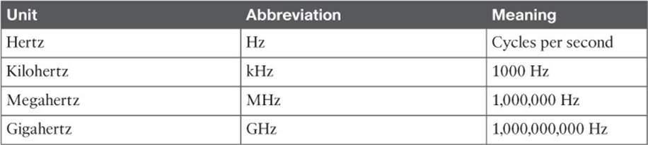
Table 1-2 Frequency Unit Names
Figure 1-6 shows a simple representation of the continuous frequency spectrum ranging from 0 Hz to 1022 (or 1 followed by 22 zeros) Hz. At the low end of the spectrum are frequencies that are too low to be heard by the human ear, followed by audible sounds. The highest range of frequencies contains light, followed by X, gamma, and cosmic rays.
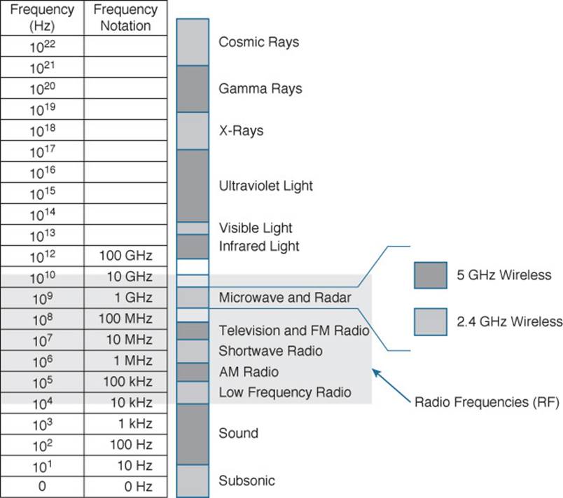
Figure 1-6 Continuous Frequency Spectrum
The frequency range from around 3 kHz to 300 GHz is commonly called radio frequency (RF). It includes many different types of radio communication, including low-frequency radio, AM radio, shortwave radio, television, FM radio, microwave, and radar. The microwave category also contains the two main frequency ranges that are used for wireless LAN communication: 2.4 and 5 GHz.
Because a range of frequencies might be used for the same purpose, it is customary to refer to the range as a band of frequencies. For example, the range from 530 kHz to around 1710 kHz is used by AM radio stations; therefore it is commonly called the AM band or the AM broadcast band.
One of the two main frequency ranges used for wireless LAN communication lies between 2.400 and 2.4835 GHz. This is usually called the 2.4-GHz band, even though it does not encompass the entire range between 2.4 and 2.5 GHz. It is much more convenient to refer to the band name instead of the specific range of frequencies included.
The other wireless LAN range is usually called the 5-GHz band because it lies between 5.150 and 5.825 GHz. The 5-GHz band actually contains the following four separate and distinct bands:
5.150 to 5.250 GHz
5.250 to 5.350 GHz
5.470 to 5.725 GHz
5.725 to 5.825 GHz
Tip
You might have noticed that most of the 5-GHz bands are contiguous except for a gap between 5.350 and 5.470. At the time of this writing, this gap exists and cannot be used for wireless LANs. However, some governmental agencies have moved to reclaim the frequencies and repurpose them for wireless LANs. Efforts are also underway to add 5.825 through 5.925 GHz.
It is interesting that the 5-GHz band can contain several smaller bands. Remember that the term band is simply a relative term that is used for convenience. At this point, do not worry about memorizing the band names or exact frequency ranges; Chapter 2 covers this in more detail.
A frequency band contains a continuous range of frequencies. If two devices require a single frequency for a wireless link between them, which frequency can they use? Beyond that, how many unique frequencies can be used within a band?
To keep everything orderly and compatible, bands are usually divided up into a number of distinct channels. Each channel is known by a channel number and is assigned to a specific frequency. As long as the channels are defined by a national or international standards body, they can be used consistently in all locations.
For example, Figure 1-7 shows the channel assignment for the 2.4-GHz band that is used for wireless LAN communication. The band contains 14 channels numbered 1 through 14, each assigned a specific frequency. First, notice how much easier it is to refer to channel numbers than the frequencies. Second, notice that the channels are spaced at regular intervals that are 0.005 GHz (or 5 MHz) apart, except for channel 14. The channel spacing is known as the channel separation or channel width.

Figure 1-7 Example of Channel Spacing in the 2.4-GHz Band
If devices use a specific frequency for a wireless link, why do the channels need to be spaced apart at all? The reason lies with the practical limitations of RF signals, the electronics involved in transmitting and receiving the signals, and the overhead needed to add data to the signal effectively.
In practice, an RF signal is not infinitely narrow; instead, it spills above and below a center frequency to some extent, occupying neighboring frequencies, too. It is the center frequency that defines the channel location within the band. The actual frequency range needed for the transmitted signal is known as the signal bandwidth, as shown in Figure 1-8. As its name implies, bandwidth refers to the width of frequency space required within the band. For example, a signal with a 22-MHz bandwidth is bounded at 11 MHz above and below the center frequency. In wireless LANs, the signal bandwidth is defined as part of a standard. Even though the signal might extend farther above and below the center frequency than the bandwidth allows, wireless devices will use something called a spectral mask to ignore parts of the signal that fall outside the bandwidth boundaries.
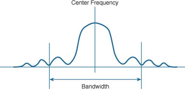
Figure 1-8 Signal Bandwidth
Ideally, the signal bandwidth should be less than the channel width so that a different signal could be transmitted on every possible channel with no chance that two signals could overlap and interfere with each other. Figure 1-9 shows such a channel spacing, where the signals on adjacent channels do not overlap. A signal can exist on every possible channel without overlapping with others.
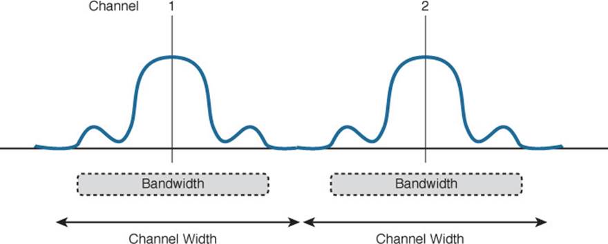
Figure 1-9 Non-overlapping Channel Spacing
However, you should not assume that signals centered on the standardized channel assignments will not overlap with each other. It is entirely possible that the channels in a band are narrower than the signal bandwidth, as shown in Figure 1-10. Notice how two signals have been centered on adjacent channel numbers 1 and 2, but they almost entirely overlap each other! The problem is that the signal bandwidth is slightly wider than four channels. In this case, signals centered on adjacent channels cannot possibly coexist without overlapping and interfering. Instead, the signals must be placed on more distant channels to prevent overlapping, thus limiting the number of channels that can be used in the band.
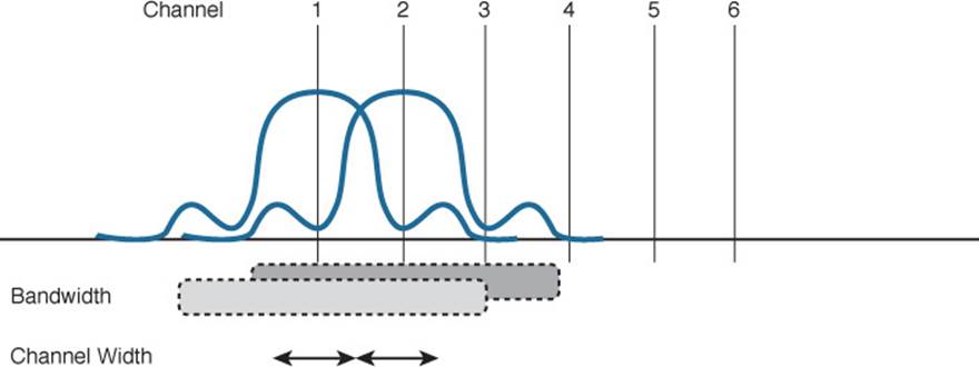
Figure 1-10 Overlapping Channel Spacing
Tip
How can channels be numbered such that signals overlap? Sometimes the channels in a band are defined and numbered for a specific use. Later on, another technology might be developed to use the same band and channels, only the newer signals might require more bandwidth than the original channel numbering supported. Such is the case with the 2.4-GHz Wi-Fi band.
Understanding Phase
RF signals are very dependent upon timing because they are always in motion. By their very nature, the signals are made up of electrical and magnetic forces that vary over time. The phase of a signal is a measure of shift in time relative to the start of a cycle. Phase is normally measured in degrees, where 0 degrees is at the start of a cycle, and one complete cycle equals 360 degrees. A point that is halfway along the cycle is at the 180-degree mark. Because an oscillating signal is cyclic, you can think of the phase traveling around a circle again and again.
When two identical signals are produced at exactly the same time, their cycles match up and they are said to be in phase with each other. If one signal is delayed from the other, the two signals are said to be out of phase. Figure 1-11 shows examples of both scenarios.
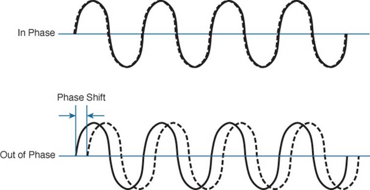
Figure 1-11 Signals In and Out of Phase
Phase becomes important as RF signals are received. Signals that are in phase tend to add together, whereas signals that are 180 degrees out of phase tend to cancel each other out. Chapter 3, “RF Signals in the Real World,” explores signal phase in greater detail.
Measuring Wavelength
RF signals are usually described by their frequency; however, it is difficult to get a feel for their physical size as they move through free space. The wavelength is a measure of the physical distance that a wave travels over one complete cycle. Wavelength is usually designated by the Greek symbol lambda (λ). To get a feel for the dimensions of a wireless LAN signal, assuming you could see it as it travels in front of you, a 2.4-GHz signal would have a wavelength of 4.92 inches, while a 5-GHz signal would be 2.36 inches.
Figure 1-12 shows the wavelength of three different waves. The waves are arranged in order of increasing frequency, from top to bottom. Regardless of the frequency, RF waves travel at a constant speed. In a vacuum, radio waves travel at exactly the speed of light; in air, the velocity is slightly less than the speed of light. Notice that the wavelength decreases as the frequency increases. As the wave cycles get smaller, they cover less distance. Wavelength becomes useful in the design and placement of antennas.
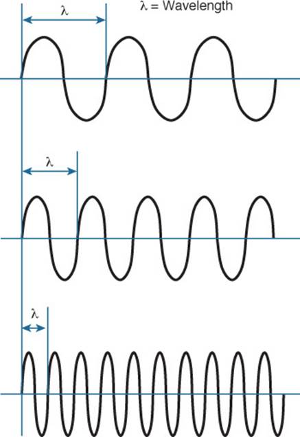
Figure 1-12 Examples of Increasing Frequency and Decreasing Wavelength
Understanding RF Power and dB
For an RF signal to be transmitted, propagated through free space, received, and understood with any certainty, it must be sent with enough strength or energy to make the journey. Think about Figure 1-1 again, where the two people are trying to signal each other with a rope. If the sender continuously moves his arm up and down a small distance, he will produce a wave in the rope. However, the wave will dampen out only a short distance away because of factors such as the weight of the rope, gravity, and so on. To move the wave all the way down the rope to reach the receiver, the sender must move his arm up and down with a much greater range of motion and with greater force or strength.
This strength can be measured as the amplitude, or the height from the top peak to the bottom peak of the signal’s waveform, as shown in Figure 1-13.
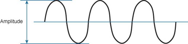
Figure 1-13 Signal Amplitude
The strength of an RF signal is usually measured by its power, in watts (W). For example, a typical AM radio station broadcasts at a power of 50,000 W; an FM radio station might use 16,000 W. In comparison, a wireless LAN transmitter usually has a signal strength between 0.1 W (100 mW) and 0.001 W (1 mW).
When power is measured in watts or milliwatts, it is considered to be an absolute power measurement. In other words, something has to measure exactly how much energy is present in the RF signal. This is fairly straightforward when the measurement is taken at the output of a transmitter because the transmit power level is usually known ahead of time.
Sometimes you might need to compare the power level between two different transmitters. For example, suppose that device T1 is transmitting at 1 mW, while T2 is transmitting at 10 mW, as shown in Figure 1-14. Simple subtraction tells you that T2 is 9 mW stronger than T1. You might also notice that T2 is 10 times stronger than T1.
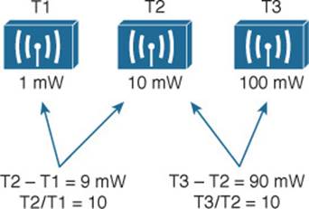
Figure 1-14 Comparing Power Levels Between Transmitters
Now compare transmitters T2 and T3, which use 10 mW and 100 mW, respectively. Using subtraction, T2 and T3 differ by 90 mW, but T3 is again 10 times stronger than T2. In each instance, subtraction yields a different result than division. Which method should you use?
Quantities like absolute power values can differ by orders of magnitude. A more surprising example is shown in Figure 1-15, where T4 is 0.00001 mW and T5 is 10 mW. Subtracting the two values gives their difference as 9.99999 mW. However, T5 is 1,000,000 times stronger than T4!
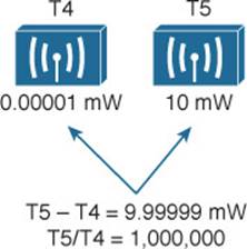
Figure 1-15 Comparing Power Levels That Differ By Orders of Magnitude
Because absolute power values can fall anywhere within a huge range, from a tiny decimal number to hundreds, thousands, or greater values, we need a way to transform the exponential range into a linear one. The logarithm function can be leveraged to do just that. In a nutshell, a logarithm takes values that are orders of magnitude apart (0.001, 0.01, 0.1, 1, 10, 100, and 1000, for example) and spaces them evenly within a reasonable range.
Tip
The base-10 logarithm function, denoted by log10, computes how many times 10 can be multiplied by itself to equal a number. For example, log10(10) equals 1 because 10 is used only once to get the result of 10. The log10(100) equals 2 because 10 is multiplied twice (10 × 10), to reach the result of 100. Computing other log10 values is difficult, requiring the use of a calculator. The good news is that you will not need a calculator or a logarithm on the CCNA Wireless exam. Even so, try to suffer through the few equations in this chapter so that you get a better understanding of power comparisons and measurements.
![]()
The decibel (dB) is a handy function that uses logarithms to compare one absolute measurement to another. It was originally developed to compare sound intensity levels, but it applies directly to power levels, too. After each power value has been converted to the same logarithmic scale, the two values can be subtracted to find the difference. The following equation is used to calculate a dB value, where P1 and P2 are the absolute power levels of two sources:
dB = 10(log10P2 – log10P1)
P2 represents the source of interest, and P1 is usually called the reference value or the source of comparison.
The difference between the two logarithmic functions can be rewritten as a single logarithm of P2 divided by P1, as follows:
![]()
Here, the ratio of the two absolute power values is computed first; then the result is converted onto a logarithmic scale.
Oddly enough, we end up with the same two methods to compare power levels with dB: a subtraction and a division. Thanks to the logarithm, both methods arrive at identical dB values. Be aware that the ratio or division form of the equation is the most commonly used in the wireless engineering world.
Important dB Laws to Remember
![]()
There are three cases where you can use mental math to make power-level comparisons using dB. By adding or subtracting fixed dB amounts, you can compare two power levels through multiplication or division. You should memorize the following three laws, with are based on dB changes of 0, 3, and 10, respectively, and are known as the Law of Zero, Law of 3s, and Law of 10s. You will be tested on them in the CCNA Wireless exam. All other dB cases require a calculator, so you will not be tested on those.
![]() Law of Zero—A value of 0 dB means that the two absolute power values are equal.
Law of Zero—A value of 0 dB means that the two absolute power values are equal.
If the two power values are equal, the ratio inside the logarithm is 1, and the log10(1) is 0. This law is intuitive; if two power levels are the same, one is 0 dB more than the other.
![]() Law of 3s—A value of 3 dB means that the power value of interest is double the reference value; a value of –3 dB means the power value of interest is half the reference.
Law of 3s—A value of 3 dB means that the power value of interest is double the reference value; a value of –3 dB means the power value of interest is half the reference.
When P2 is twice P1, the ratio is always 2. Therefore, 10log10(2) = 3 dB.
When the ratio is 1/2, 10log10(1/2) = –3 dB.
The Law of 3s is not very intuitive, but is still easy to learn. Whenever a power level doubles, it increases by 3 dB. Whenever it is cut in half, it decreases by –3 dB.
![]() Law of 10s—A value of 10 dB means that the power value of interest is 10 times the reference value; a value of –10 dB means the power value of interest is 1/10 of the reference.
Law of 10s—A value of 10 dB means that the power value of interest is 10 times the reference value; a value of –10 dB means the power value of interest is 1/10 of the reference.
When P2 is 10 times P1, the ratio is always 10. Therefore, 10log10(10) = 10 dB.
When P2 is one tenth of P1, then the ratio is 1/10 and 10log10(1/10) = –10 dB.
The Law of 10s is intuitive because multiplying or dividing by 10 adds or subtracts 10 dB, respectively.
Notice another handy rule of thumb: When absolute power values multiply, the dB value is positive and can be added. When the power values divide, the dB value is negative and can be subtracted. Table 1-3 summarizes the useful dB comparisons.
![]()
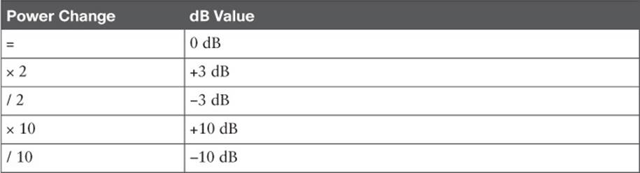
Table 1-3 Power Changes and Their Corresponding dB Values
Try a few example problems to see whether you understand how to compare two power values using dB. In Figure 1-16, sources A, B, and C transmit at 4, 8, and 16 mW, respectively. Source B is double the value of A, so it must be 3 dB greater than A. Likewise, source C is double the value of B, so it must be 3 dB greater than B.
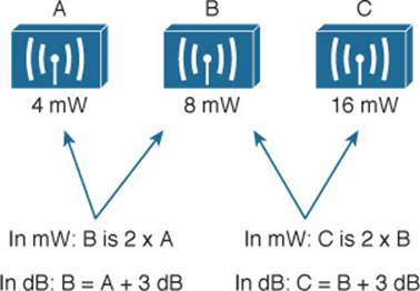
Figure 1-16 Comparing Power Levels Using dB
You can also compare sources A and C. To get from A to C, you have to double A, and then double it again. Each time you double a value, just add 3 dB. Therefore, C is 3 dB + 3 dB = 6 dB greater than A.
Next, try the more complicated example shown in Figure 1-17. Keep in mind that dB values can be added and subtracted in succession (in case several multiplication and division operations involving 2 and 10 are needed).
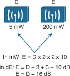
Figure 1-17 Example of Computing dB with Simple Rules
Sources D and E have power levels 5 and 200 mW. Try to figure out a way to go from 5 to 200 using only ×2 or ×10 operations. You can double 5 to get 10, then double 10 to get 20, and then multiply by 10 to reach 200 mW. Next, use the dB laws to replace the doubling and ×10 with the dB equivalents. The result is E = D + 3 + 3 + 10 or E = D + 16 dB.
You might also find other ways to reach the same result. For example, you can start with 5 mW, then multiply by 10 to get 50, then double 50 to get 100, then double 100 to reach 200 mW. This time the result is E = D + 10 + 3 + 3 or E = D + 16 dB.
Comparing Power Against a Reference: dBm
Beyond comparing two transmitting sources, a wireless LAN engineer must be concerned about the RF signal propagating from a transmitter to a receiver. After all, transmitting a signal is meaningless unless someone is there to receive it and make use of it.
Figure 1-18 shows a simple scenario with a transmitter and a receiver. Nothing in the real world is ideal, so assume that something along the path of the signal will induce a net loss. At the receiver, the signal strength will be degraded by some amount. Suppose that you are able to measure the power level leaving the transmitter, which is 100 mW. At the receiver, you measure the power level of the arriving signal. It is an incredibly low 0.000031623 mW.
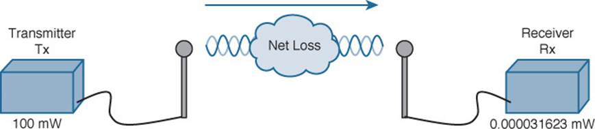
Figure 1-18 Example of RF Signal Power Loss
Wouldn’t it be nice to quantify the net loss over the signal’s path? After all, you might want to try several other transmit power levels or change something about the path between the transmitter and receiver. To design the signal path properly, you would like to make sure that the signal strength arriving at the receiver is at an optimum level.
You could leverage the handy dB formula to compare the received signal strength to the transmitted signal strength, as long as you can remember the formula and have a calculator nearby:
![]()
The net loss over the signal path turns out to be a decrease of 65 dB. Knowing that, you decide to try a different transmit power level to see what would happen at the receiver. It does not seem very straightforward to use the new transmit power to find the new signal strength at the receiver. That might require more formulas and more time at the calculator.
A better approach is to compare each absolute power along the signal path to one common reference value. Then, regardless of the absolute power values, you could just focus on the changes to the power values that are occurring at various stages along the signal path. In other words, convert every power level to a dB value and simply add them up along the path.
Recall that the dB formula puts the power level of interest on the top of the ratio, with a reference power level on the bottom. In wireless networks, the reference power level is usually 1 mW, so the units are designated by dBm (dB-milliwatt).
Returning to the scenario from Figure 1-18, the absolute power values at the transmitter and receiver can be converted to dBm, the results from which are shown in Figure 1-19. Notice that the dBm values can be added along the path: The transmitter dBm plus the net loss in dB equals the received signal in dBm.
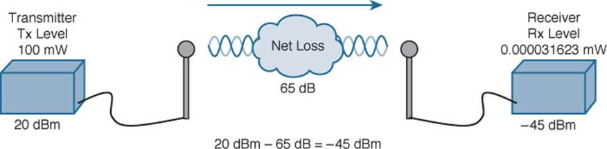
Figure 1-19 Subtracting dB to Represent a Loss in Signal Strength
Measuring Power Changes Along the Signal Path
Up to this point, this chapter has considered a transmitter and its antenna to be a single unit. That might seem like a logical assumption because many wireless access points have built-in antennas. In reality, a transmitter, its antenna, and the cable that connects them are all discrete components that not only propagate an RF signal but also affect its absolute power level.
When an antenna is connected to a transmitter, it provides some amount of gain to the resulting RF signal. This effectively increases the dB value of the signal above that of the transmitter alone. Chapter 4 explains this in greater detail; for now, just be aware that antennas provide positive gain.
By itself, an antenna does not generate any amount of absolute power. In other words, when an antenna is disconnected, no milliwatts of power are being pushed out of it. That makes it impossible to measure the antenna’s gain in dBm. Instead, an antenna’s gain is measured by comparing its performance with that of a reference antenna, then computing a value in dB.
Usually, the reference antenna is an isotropic antenna, so the gain is measured in dBi (dB-isotropic). An isotropic antenna does not actually exist, because it is ideal in every way. Its size is a tiny point, and it radiates RF equally in every direction. No physical antenna can do that. The isotropic antenna’s performance can be calculated according to RF formulas, making it a universal reference for any antenna.
Because of the physical qualities of the cable that connects an antenna to a transmitter, some signal loss always occurs. Cable vendors supply the loss in dB per foot or meter of cable length for each type of cable manufactured.
![]()
Once you know the complete combination of transmitter power level, the length of cable, and the antenna gain, you can figure out the actual power level that will be radiated from the antenna. This is known as the effective isotropic radiated power (EIRP), measured in dBm.
EIRP is a very important parameter because it is regulated by governmental agencies in most countries. In those cases, a system cannot radiate signals higher than a maximum allowable EIRP. To find the EIRP of a system, simply add the transmitter power level to the antenna gain and subtract the cable loss, as illustrated in Figure 1-20.
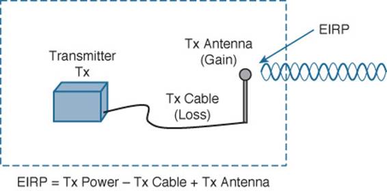
Figure 1-20 Calculating EIRP
Suppose a transmitter is configured for a power level of 10 dBm (10 mW). A cable with 5-dB loss connects the transmitter to an antenna with an 8-dBi gain. The resulting EIRP of the system is 10 dBm – 5 dB + 8 dBi, or 13 dBm.
You might notice that the EIRP is made up of decibel-milliwatt (dBm), dB relative to an isotropic antenna (dBi), and decibel (dB) values. Even though the units appear to be different, you can safely combine them for the purposes of calculating the EIRP. The only exception to this is when an antenna’s gain is measured in dBd (dB-dipole). In that case, a dipole antenna has been used as the reference antenna, rather than an isotropic antenna. A dipole is a simple actual antenna, which has a gain of 2.14 dBi. If an antenna has its gain shown as dBi, you can add 2.14 dBi to that value to get its gain in dBi units instead.
Power-level considerations do not have to stop with the EIRP. You should also be concerned with the complete path of a signal, to make sure that the transmitted signal has sufficient power so that it can effectively reach and be understood by a receiver. This is known as the link budget.
The dB values of gains and losses can be combined over any number of stages along a signal’s path. Consider Figure 1-21, which shows every component of signal gain or loss along the path from transmitter to receiver.
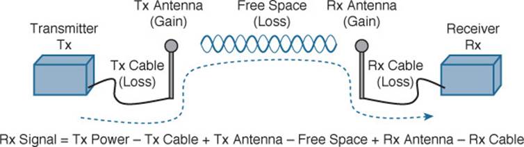
Figure 1-21 Calculating Received Signal Strength Over the Path of an RF Signal
At the receiving end, an antenna provides gain to increase the received signal power level. A cable connecting the antenna to the receiver also introduces some loss.
Figure 1-22 shows some example dB values, as well as the resulting sum of the component parts across the entire signal path. The signal begins at 20 dBm at the transmitter, has an EIRP value of 22 dBm at the transmitting antenna (20 dBm – 2 dB + 4 dBi), and arrives at the receiver with a level of –45 dBm.
Tip
Notice that every signal gain or loss used in Figure 1-22 is given except for the 69-dB loss between the two antennas. In this case, the loss can be quantified based on the other values given. In reality, it can be calculated as a function of distance and frequency. For perspective, you might see a 69-dB Wi-Fi loss over a distance of about 13 to 28 meters. Free space path loss is covered in greater detail in Chapter 3, “RF Signals in the Real World.”
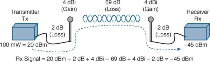
Figure 1-22 Example of Calculating Received Signal Strength
If you always begin with the transmitter power expressed in dBm, it is a simple matter to add or subtract the dB components along the signal path to find the signal strength that arrives at the receiver.
Understanding Power Levels at the Receiver
At the receiving end of the signal path, a receiver expects to find a signal on a predetermined frequency, with enough power to contain useful data. Receivers measure a signal’s power in dBm according to the received signal strength indicator (RSSI) scale.
When you work with wireless LAN devices, the EIRP levels leaving the transmitter’s antenna normally range from 100 mW down to 1 mW. This corresponds to the range +20 dBm down to 0 dBm. At the receiver, the power levels are much, much less, ranging from 1 mW all the way down to tiny fractions of a milliwatt, approaching 0 mW. The corresponding range of received signal levels is from 0 dBm down to about –100 dBm.
Therefore, the RSSI of a received signal can range from 0 to –100, where 0 is the strongest and –100 is the weakest. The range of RSSI values can vary between one hardware manufacturer and another. RSSI values are supposed to represent dBm values, but the results are not standardized across all receiver manufacturers. An RSSI value can vary from one receiver hardware to another.
Assuming a transmitter is sending an RF signal with enough power to reach a receiver, what RSSI value is good enough? Every receiver has a sensitivity level or a threshold that divides intelligible, useful signals from unintelligible ones. As long as a signal is received with a power level that is greater than the sensitivity level, chances are that the data from the signal can be understood correctly. Figure 1-23 shows an example of how the signal strength at a receiver might change over time. The receiver’s sensitivity level is –82 dBm.
![]()
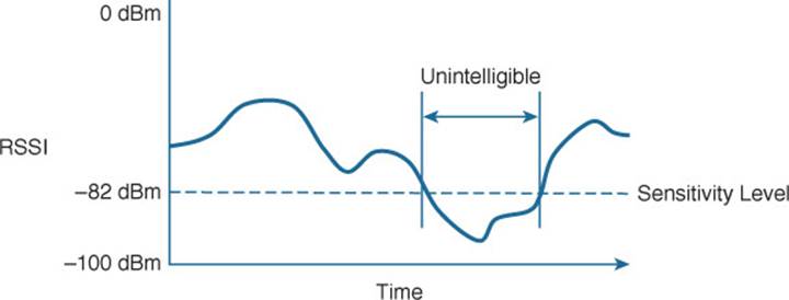
Figure 1-23 Example of Receiver Sensitivity Level
The RSSI value focuses on the expected signal alone, without regard to any other signals that may be received, too. All other signals that are received on the same frequency as the one you are trying to receive are simply viewed as noise. The noise level, or the average signal strength of the noise, is called the noise floor.
It is easy to ignore noise as long as the noise floor is well below what you are trying to hear. For example, two people can whisper in a library effectively because there is very little competing noise. Those same two people would become very frustrated if they tried to whisper to each other in a crowded sports arena.
Receiving an RF signal is no different; its signal strength must be greater than the noise floor by a decent amount so that it can be received and understood correctly. The difference between the signal and the noise is called the signal-to-noise ratio (SNR), measured in dB. A higher SNR value is preferred.
Figure 1-24 shows the RSSI of a signal compared with the noise floor that is received. The RSSI averages around –54 dBm. On the left side of the graph, the noise floor is –90 dBm. The resulting SNR is –54 dBm – (–90) dBm or 36 dB. Toward the right side of the graph, the noise floor gradually increases to –65 dBm, reducing the SNR to 11 dB. The signal is so close to the noise that it might not be usable.
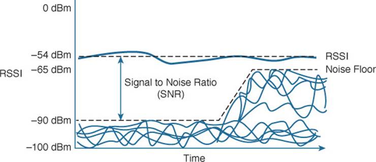
Figure 1-24 Example of a Changing Noise Floor and SNR
Carrying Data Over an RF Signal
Up to this point in the chapter, only the RF characteristics of wireless signals have been discussed. The RF signals presented have existed only as simple oscillations in the form of a sine wave. The frequency, amplitude, and phase have all been constant. The steady, predictable frequency is important because a receiver needs to tune to a known frequency to find the signal in the first place.
This basic RF signal is called a carrier signal because it is used to carry other useful information. With AM and FM radio signals, the carrier signal also transports audio signals. TV carrier signals have to carry both audio and video. Wireless LAN carrier signals must carry data.
To add data onto the RF signal, the frequency of the original carrier signal must be preserved. Therefore, there must be some scheme of altering some characteristic of the carrier signal to distinguish a 0 bit from a 1 bit. Whatever scheme is used by the transmitter must also be used by the receiver so that the data bits can be correctly interpreted.
Figure 1-25 shows a carrier signal with a constant frequency. The data bits 1001 are to be sent over the carrier signal, but how? One idea might be to simply use the value of each data bit to turn the carrier signal off or on. The Bad Idea 1 plot shows the resulting RF signal. A receiver might be able to notice when the signal is present and has an amplitude and correctly interpret 1 bits, but there is no signal to receive during 0 bits. If the signal becomes weak or is not available for some reason, the receiver will incorrectly think that a long string of 0 bits has been transmitted. A different twist might be to transmit only the upper half of the carrier signal during a 1 bit and the lower half during a 0 bit, as shown in the Bad Idea 2 plot. This time, a portion of the signal is always available for the receiver, but the signal becomes impractical to receive because important pieces of each cycle are missing. In addition, it is very difficult to transmit RF with disjointed alternating cycles.
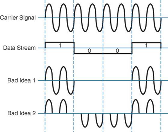
Figure 1-25 Poor Attempts at Sending Data Over an RF Signal
Such naive approaches might not be successful, but they do have the right idea: to alter the carrier signal in a way that indicates the information to be carried. This is known as modulation, where the carrier signal is modulated or changed according to some other source. At the receiver, the process is reversed; demodulation interprets the added information based on changes in the carrier signal.
RF modulation schemes generally have the following goals:
![]() Carry data at a predefined rate
Carry data at a predefined rate
![]() Be reasonably immune to interference and noise
Be reasonably immune to interference and noise
![]() Be practical to transmit and receive
Be practical to transmit and receive
Due to the physical properties of an RF signal, a modulation scheme can alter only the following attributes:
![]() Frequency, but only by varying slightly above or below the carrier frequency
Frequency, but only by varying slightly above or below the carrier frequency
![]() Phase
Phase
![]() Amplitude
Amplitude
The modulation techniques require some amount of bandwidth centered on the carrier frequency. This additional bandwidth is partly due to the rate of the data being carried and partly due to the overhead from encoding the data and manipulating the carrier signal. If the data has a relatively low bit rate, such as an audio signal carried over AM or FM radio, the modulation can be straightforward and requires little extra bandwidth. Such signals are called narrowband transmissions.
In contrast, wireless LANs must carry data at high bit rates, requiring more bandwidth for modulation. The end result is that the data being sent is spread out across a range of frequencies. This is known as spread spectrum. At the physical layer, wireless LANs can be broken down into the following three spread-spectrum categories, which are discussed in subsequent sections:
![]() Frequency-hopping spread spectrum (FHSS)
Frequency-hopping spread spectrum (FHSS)
![]() Direct-sequence spread spectrum (DSSS)
Direct-sequence spread spectrum (DSSS)
![]() Orthogonal frequency-division multiplexing (OFDM)
Orthogonal frequency-division multiplexing (OFDM)
FHSS
Early wireless LAN technology took a novel approach as a compromise between avoiding RF interference and needing complex modulation. The wireless band was divided into 79 channels or fewer, with each channel being 1 MHz wide. To avoid narrowband interference, where an interfering signal would affect only a few channels at a time, transmissions would need to continuously “hop” between frequencies all across the band. This is known as frequency-hopping spread spectrum.
Figure 1-26 shows an example of how the FHSS technique works, where the sequence begins on channel 2, then moves to channels 25, 64, 10, 45, and so on, through an entire predetermined sequence before repeating again. Hopping between channels has to occur at regular intervals so that the transmitter and receiver can stay synchronized. In addition, the hopping order must be worked out in advance so that the receiver can always tune to the correct frequency in use at any given time.
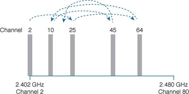
Figure 1-26 Example FHSS Channel-Hopping Sequence
Whatever advantage FHSS gained avoiding interference was lost because of the following limitations:
![]() Narrow 1-MHz channel bandwidth, limiting the data rate to 1 or 2 Mbps.
Narrow 1-MHz channel bandwidth, limiting the data rate to 1 or 2 Mbps.
![]() Multiple transmitters in an area could eventually collide and interfere with each other on the same channels.
Multiple transmitters in an area could eventually collide and interfere with each other on the same channels.
As a result, FHSS fell out of favor and was replaced by another, more robust and scalable spread-spectrum approach: DSSS. Even though FHSS is rarely used now, you should be familiar with it and its place in the evolution of wireless LAN technologies.
DSSS
Direct-sequence spread spectrum uses a small number of fixed, wide channels that can support complex modulation schemes and somewhat scalable data rates. Each channel is 22 MHz wide—a much wider bandwidth compared with the maximum supported 11-Mbps data rate, but wide enough to augment the data by spreading it out and making it more resilient to disruption. In the 2.4-GHz band where DSSS is used, there are 14 possible channels, but only 3 of them that do not overlap. Figure 1-27 shows how channels 1, 6, and 11 are normally used.
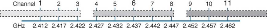
Figure 1-27 Example Non-overlapping Channels Used for DSSS
DSSS transmits data in a serial stream, where each data bit is prepared for transmission one at a time. It might seem like a simple matter to transmit the data bits in the order that they are stored or presented to the wireless transmitter; however, RF signals are often affected by external factors like noise or interference that can garble the data at the receiver. For that reason, a wireless transmitter performs several functions to make the data stream less susceptible to being degraded along the transmission path:
![]() Scrambler—The data waiting to be sent is first scrambled in a predetermined manner so that it becomes a randomized string of 0 and 1 bits rather than long sequences of 0 or 1 bits.
Scrambler—The data waiting to be sent is first scrambled in a predetermined manner so that it becomes a randomized string of 0 and 1 bits rather than long sequences of 0 or 1 bits.
![]() Coder—Each data bit is converted into multiple bits of information that contain carefully crafted patterns that can be used to protect against errors due to noise or interference. Each of the new coded bits is called a chip. The complete group of chips representing a data bit is called asymbol. DSSS uses two encoding techniques: Barker codes and Complementary Code Keying (CCK).
Coder—Each data bit is converted into multiple bits of information that contain carefully crafted patterns that can be used to protect against errors due to noise or interference. Each of the new coded bits is called a chip. The complete group of chips representing a data bit is called asymbol. DSSS uses two encoding techniques: Barker codes and Complementary Code Keying (CCK).
![]() Interleaver—The coded data stream of symbols is spread out into separate blocks so that bursts of interference might affect one block, but not many.
Interleaver—The coded data stream of symbols is spread out into separate blocks so that bursts of interference might affect one block, but not many.
![]() Modulator—The bits contained in each symbol are used to alter or modulate the phase of the carrier signal. This enables the RF signal to carry the binary data bit values.
Modulator—The bits contained in each symbol are used to alter or modulate the phase of the carrier signal. This enables the RF signal to carry the binary data bit values.
Figure 1-28 shows the entire data preparation process. At the receiver, the entire process is reversed. The DSSS techniques discussed in this chapter focus only on the coder and modulator functions.
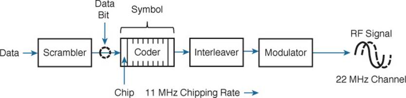
Figure 1-28 Functional Blocks Used in a DSSS Transmitter
DSSS has evolved over time to increase the data rate that is modulated onto the RF signal. The following sections describe each DSSS method and data rate, in progression. Regardless of the data rate, DSSS always uses a chipping rate of 11 million chips per second.
1-Mbps Data Rate
To minimize the effect of a low SNR and data loss in cases of narrowband interference, each bit of data is encoded as a sequence of 11 bits called a Barker 11 code. The goal is to add enough additional information to each bit of data that its integrity will be preserved when it is sent in a noisy environment.
It might seem ridiculous to turn 1 bit into 11 bits. As an analogy, voice transmissions over an RF signal can be subject to noise and interference, too. Spelling words letter by letter can help, but even single letters can become garbled and ambiguous. For example, the letters B, C, D, E, G, P, T,V, and Z can all sound similar when noise is present. Phonetic alphabets have been developed to remove the ambiguity. Instead of saying the letter B, the word Bravo is spoken; C becomes Charlie, D becomes Delta, and so on. Replacing single letters with longer, unique words makes the listener’s job much easier and more accurate.
There are only two possible values for the Barker chips—one corresponding to a 0 data bit (10110111000) and one for a 1 data bit (01001000111). The receiver must also expect the Barker chips and convert them back into single bits of data. The number and sequence of the Barker chip bits have been defined to allow data bits to be recovered if some of the chip bits are lost. In fact, up to 9 of the 11 bits in a single chip can be lost before the original data bit cannot be restored.
Each bit in a Barker chip can be transmitted by using the differential binary phase shift keying (DBPSK) modulation scheme. The phase of the carrier signal is shifted or rotated according to the data bit being transmitted, as follows:
0: The phase is not changed.
1: The phase is “rotated” or shifted 180 degrees, such that the signal is suddenly inverted.
DBPSK can modulate 1 bit of data at a time onto the RF signal. With a steady chipping rate of 11 million chips per second, where each symbol (1 original bit) contains 11 chips, the transmitted data rate is 1 Mbps.
2-Mbps Data Rate
It is possible to couple the 1-Mbps strategy with a different modulation scheme to double the data rate. As before, each data bit is coded into an 11-bit Barker code with an 11-MHz chipping rate. This time, chips are taken two at a time and modulated onto the carrier signal by usingdifferential quadrature phase shift keying (DQPSK). The two chips are used to affect the carrier signal’s phase in four possible ways, each one 90 degrees apart (hence, the name quadrature). The bit patterns produce the following phase shifts:
![]() 00—The phase is not changed.
00—The phase is not changed.
![]() 01—Rotate the phase 90 degrees.
01—Rotate the phase 90 degrees.
![]() 11—Rotate the phase 180 degrees.
11—Rotate the phase 180 degrees.
![]() 10—Rotate the phase 270 degrees.
10—Rotate the phase 270 degrees.
Because DQPSK can modulate data bits in pairs, it is able to transmit twice the data rate of DBPSK, or 2 Mbps.
Figure 1-29 shows examples of DBPSK and DQPSK modulation. Each input data bit combination is shown along with the carrier signal phase rotation that occurs. Phase rotations can occur at several points along a cycle; for simplicity, only rotations at the beginning of the cycle (0 degrees) are shown. Notice how abrupt the phase can change, according to the bits being modulated. The receiver must detect these phase changes when it demodulates the signal so that the original data bits can be recovered.
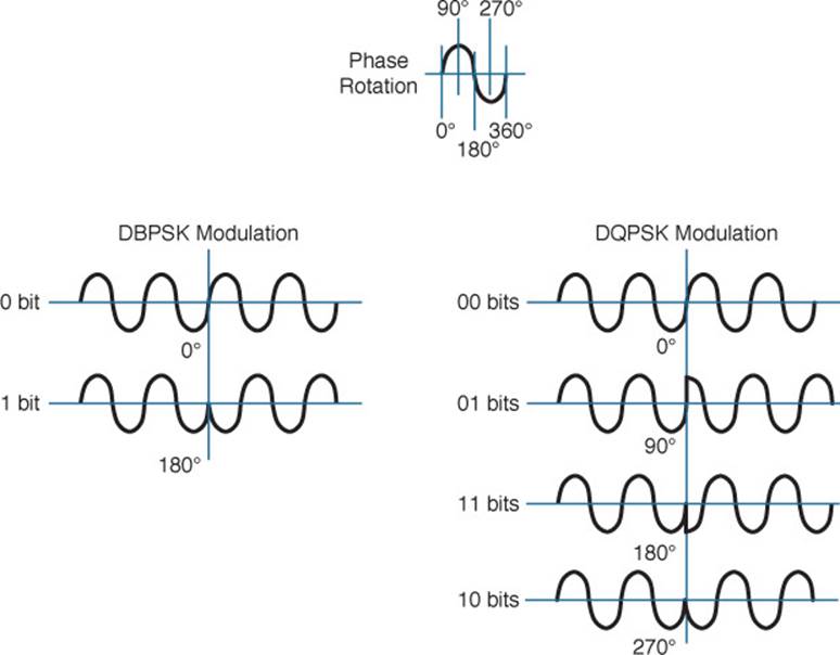
Figure 1-29 Example Phase Changes During DBPSK and DQPSK Modulation
Tip
As you read about wireless modulation techniques, you will often see terms like DBPSK and BPSK mentioned. The two forms reference the same type of modulation (BPSK, in this case), but differ in the reference signal that the receiver uses to detect the phase changes. The nondifferential form (without the initial D) means the receiver must compare with the original premodulated signal to find phase changes. The differential form (with the D) means the receiver must figure out phase changes by comparing with previous phases already seen in the received signal.
5.5-Mbps Data Rate
To gain more efficiency, Complementary Code Keying (CCK) can replace the Barker code. CCK can take 4 bits of data at a time and build out redundant information to create a unique 6-chip symbol. Two more bits are added to indicate the modulated phase orientation for the symbol, resulting in 8 chips total. CCK is naturally coupled with DQPSK modulation; the two-phase orientation bits determine four possible carrier signal phase rotation values.
The chipping rate remains steady at 11 MHz, but each symbol contains 8 chips. This results in a symbol rate of 1.375 MHz. Each symbol is based on 4 original data bits, so the effective data rate is 5.5 Mbps.
11-Mbps Data Rate
The 5.5-Mbps CCK data rate can be doubled by making an adjustment to the coder. Instead of taking 4 data bits at a time to make each coder symbol, data can be taken 8 bits at a time to create a unique 8-chip symbol. The CCK symbol rate is still 1.375 MHz, so 8 data bits per symbol results in a data rate of 11 Mbps.
The smaller 8-chip CCK symbol is more efficient than the 11-bit Barker code because more data bits can be sent with each new symbol. At the same time, CCK loses some of the extra bits used by the Barker code to recover information received in a noisy or low SNR environment. In other words, CCK achieves faster data rates at the expense of requiring a stronger, less-noisy signal.
OFDM
DSSS spreads the chips of a single data stream into one wide, 22-MHz channel. It is inherently limited to an 11-Mbps data rate because of the consistent 11-MHz chipping rate that feeds into the RF modulation. To scale beyond that limit, a vastly different approach is needed.
In contrast, orthogonal frequency-division multiplexing (OFDM) sends data bits in parallel over multiple frequencies, all contained in a single 20-MHz channel. Each channel is divided into 64 subcarriers (also called subchannels or tones) that are spaced 312.5 kHz apart. The subcarriers are broken down into the following types:
![]() Guard—12 subcarriers are used to help set one channel apart from another and to help receivers lock onto the channel.
Guard—12 subcarriers are used to help set one channel apart from another and to help receivers lock onto the channel.
![]() Pilot—4 subcarriers are equally spaced and always transmitted to help receivers evaluate the noise state of the channel.
Pilot—4 subcarriers are equally spaced and always transmitted to help receivers evaluate the noise state of the channel.
![]() Data—48 subcarriers are devoted to carrying data.
Data—48 subcarriers are devoted to carrying data.
Tip
Sometimes you might see OFDM described as having 52 subcarriers (48 for data and 4 for pilot). This is because the 12 guard frequencies are not actually transmitted, but stay silent as channel spacing.
Figure 1-30 shows an example of OFDM, where channel 6 in the 2.4-GHz band is 20 MHz wide with 48 data subcarriers. OFDM is named for the way it takes one channel and divides it into a set of distinct frequencies for its subcarriers. Notice that the subcarriers appear to be spaced too close together, causing them to overlap. In fact, that is the case, but instead of interfering with each other, the overlapped portions are aligned so that they cancel most of the potential interference.
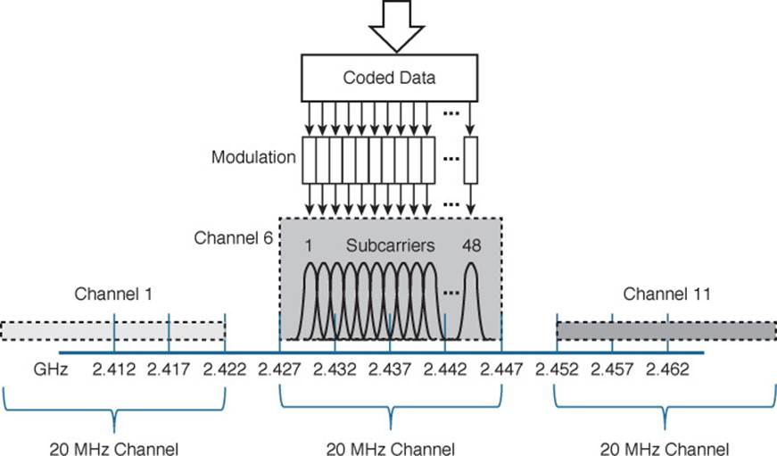
Figure 1-30 OFDM Operation with 48 Parallel Subcarriers
OFDM has the usual scrambling, coding, interleaving, and modulating functions, but it gains its scalability by leveraging so many data subcarriers in parallel. Even though the data rates through each subcarrier are relatively low, the sum of all subcarriers results in a high aggregate data rate.
OFDM offers many different data rates through several different modulation schemes. Because OFDM is concerned with moving data in parallel at higher rates, the amount of information that is repeated for resilience can be varied. The coders used with OFDM are named according to the fraction of symbols that are new or unique, and not repeated. For example, BPSK 1/2 designates that one half of the bits are new and one half are repeated. BPSK 3/4 uses a coder that presents three-fourths new data and repeats only one fourth. As a rule of thumb, a greater fraction means a greater data rate, but a lower tolerance for errors.
At the low end of the range, the familiar BPSK modulation can be used along with two different coder ratios. In this case, OFDM still uses 48 subchannels or tones, with a reduced tone rate of 250 Kbps. OFDM with BPSK 1/2 results in a 6-Mbps data rate, whereas BPSK 3/4 gives 9 Mbps. QPSK 1/2 and 3/4 can be used to increase the data rate to 12 and 18 Mbps, respectively.
Recall that QPSK uses 2 data bits to modulate the RF signal, resulting in four possible phase shifts. To achieve data rates greater than 18 Mbps, more bits must be used to modulate the signal. Quadrature amplitude modulation (QAM) combines QPSK phase shifting (quadrature) with multiple amplitude levels to get a greater number of unique alterations to the signal. For example, 16-QAM uses 2 bits to select the QPSK phase rotation and 2 bits to select the amplitude level, giving 4 bits or 16 unique modulation changes. Figure 1-31 illustrates a 16-QAM operation.
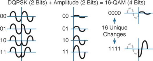
Figure 1-31 Examples of Phase and Amplitude Changes with 16-QAM
The number of possible outcomes is always given as a prefix to the QAM name, followed by the coder ratio of new data. In other words, 16-QAM is available in 1/2 and 3/4, providing data rates of 24 and 36 Mbps, respectively. Beyond that, 64-QAM uses 8 phase shifts and 8 amplitude levels to produce 64 unique modulation changes. The 64-QAM 2/3 and 64-QAM 3/4 methods offer 48 and 54 Mbps, respectively.
The same scheme is extended even further with 256-QAM 3/4 and 256-QAM 5/6. As the 256 prefix denotes, 16 different phase shifts and 16 different amplitude levels are combined to produce 256 unique modulation changes, effectively encoding 8 bits of data at a time. With so many shifts and levels in use, receivers can have a difficult job determining the original transmitted values accurately—especially when noise is present. As the modulation schemes get more complex (the QAM prefix gets higher), the signal-to-noise ratio must become greater.
Modulation Summary
Table 1-4 lists all the modulation techniques used in wireless LANs. There are quite a few, and you will have to know them all for the CCNA Wireless exam. The modulation types are broken down by DSSS and OFDM. This will become important as wireless standards are introduced inChapter 2.
![]()
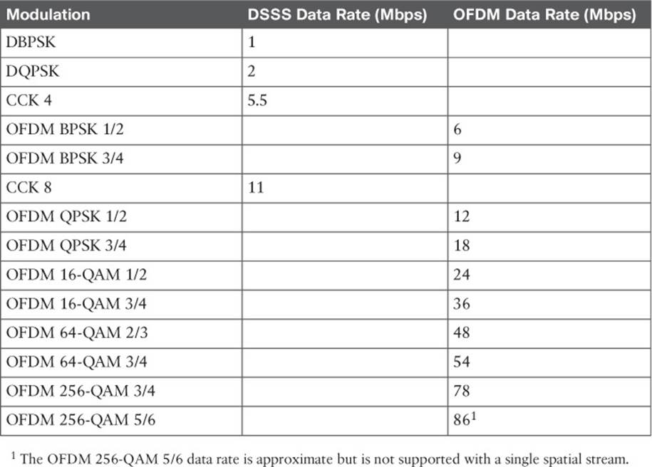
Table 1-4 Wireless LAN Modulation Techniques
Try to get a feel for the relative data rates, working from the lowest to the highest. Remember that
![]() B in DBPSK stands for binary (two outcomes).
B in DBPSK stands for binary (two outcomes).
![]() Q in DQPSK stands for quadrature (four outcomes).
Q in DQPSK stands for quadrature (four outcomes).
![]() CCK is coupled with QPSK and replaces Barker 11 to go a bit faster.
CCK is coupled with QPSK and replaces Barker 11 to go a bit faster.
![]() OFDM generally wins out, except at the two slowest BPSK methods, which sit between the two CCK methods.
OFDM generally wins out, except at the two slowest BPSK methods, which sit between the two CCK methods.
![]() QAM leverages both phase and amplitude changes to move the greatest amount of data.
QAM leverages both phase and amplitude changes to move the greatest amount of data.
![]() Higher fractions mean higher data rates.
Higher fractions mean higher data rates.
To pass data over an RF signal successfully, both a transmitter and receiver have to use the same modulation method. In addition, the pair should use the best data rate possible, given their current environment. If they are located in a noisy environment, where a low SNR or a low RSSI might result, a lower data rate might be preferable. If not, a higher data rate is better.
With so many possible modulation methods available, how do the transmitter and receiver select a common method to use? To complicate things, the transmitter, the receiver, or both might be mobile. As they move around, the SNR and RSSI conditions will likely change from one moment to the next. The most effective approach is to have the transmitter and receiver negotiate a modulation method (and the resulting data rate) dynamically, based on current RF conditions.
Chapter 2 explains the industry standards that are used in wireless LANs and how they influence the modulation techniques that are used.
Exam Preparation Tasks
As mentioned in the section “How to Use This Book” in the Introduction, you have a couple of choices for exam preparation: the exercises here, Chapter 21, “Final Review,” and the exam simulation questions on the DVD.
Review All Key Topics
Review the most important topics in this chapter, noted with the Key Topic icon in the outer margin of the page. Table 1-5 lists a reference of these key topics and the page numbers on which each is found.
![]()
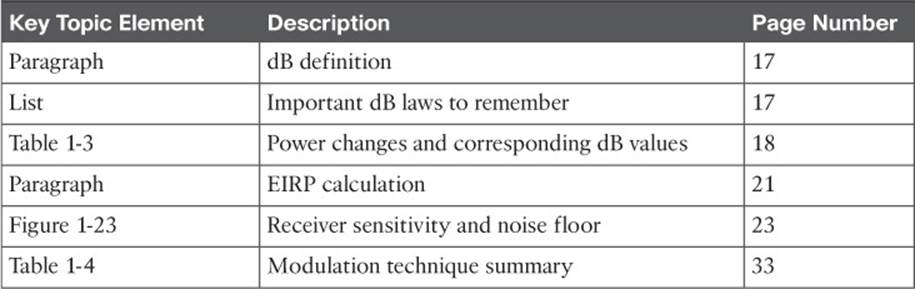
Table 1-5 Key Topics for Chapter 1
Key Terms
Define the following key terms from this chapter and check your answers in the glossary:
amplitude
band
bandwidth
Barker code
carrier signal
channel
chip
coder
Complementary Code Keying (CCK)
decibel (dB)
dBd
dBi
dBm
demodulation
differential binary phase shift keying (DBPSK)
differential quadrature phase shift keying (DQPSK)
direct-sequence spread spectrum (DSSS)
effective isotropic radiated power (EIRP)
frequency
frequency-hopping spread spectrum (FHSS)
hertz (Hz)
in phase
isotropic antenna
link budget
modulation
narrowband
noise floor
orthogonal frequency-division multiplexing (OFDM)
out of phase
phase
quadrature amplitude modulation (QAM)
radio frequency (RF)
received signal strength indicator (RSSI)
sensitivity level
signal-to-noise ratio (SNR)
spread spectrum
symbol
wavelength
tures.
All materials on the site are licensed Creative Commons Attribution-Sharealike 3.0 Unported CC BY-SA 3.0 & GNU Free Documentation License (GFDL)
If you are the copyright holder of any material contained on our site and intend to remove it, please contact our site administrator for approval.
© 2016-2026 All site design rights belong to S.Y.A.