CCNP Routing and Switching ROUTE 300-101 Official Cert Guide (2015)
Part III. Route Redistribution and Selection
Chapter 11. Route Selection
This chapter covers the following subjects:
![]() Cisco Express Forwarding: This section discusses how a router performs packet switching, primarily focusing on Cisco Express Forwarding (CEF).
Cisco Express Forwarding: This section discusses how a router performs packet switching, primarily focusing on Cisco Express Forwarding (CEF).
![]() Policy-Based Routing: This section describes the Cisco IOS Policy-Based Routing (PBR) feature, which allows a router to make packet-forwarding decisions based on criteria other than the packet’s destination address as matched with the IP routing table.
Policy-Based Routing: This section describes the Cisco IOS Policy-Based Routing (PBR) feature, which allows a router to make packet-forwarding decisions based on criteria other than the packet’s destination address as matched with the IP routing table.
![]() IP Service-Level Agreement: This section gives a general description of the IP Service-Level Agreement (IP SLA) feature, with particular attention to how it can be used to influence when a router uses a static route and when a router uses PBR.
IP Service-Level Agreement: This section gives a general description of the IP Service-Level Agreement (IP SLA) feature, with particular attention to how it can be used to influence when a router uses a static route and when a router uses PBR.
![]() VRF-Lite: This section demonstrates a basic configuration of VRF-Lite, which allows a single physical router to run multiple virtual router instances, thereby providing network segmentation.
VRF-Lite: This section demonstrates a basic configuration of VRF-Lite, which allows a single physical router to run multiple virtual router instances, thereby providing network segmentation.
The term path control can mean a variety of things, depending on the context. The typical use of the term refers to any and every function that influences where a router forwards a packet. With that definition, path control includes practically every topic in this book. In other cases, the termpath control refers to tools that influence the contents of a routing table, usually referring to routing protocols.
This chapter examines three path control topics that fit only into the broader definition of the term. The first, Cisco Express Forwarding (CEF), is a feature that allows a router to very quickly and efficiently make a route lookup. This chapter contrasts CEF with a couple of its predecessors,Process Switching and Fast Switching.
The second major topic in this chapter is Policy-Based Routing (PBR), sometimes called Policy Routing. PBR influences the IP data plane, changing the forwarding decision a router makes, but without first changing the IP routing table.
Then, this chapter turns its attention to the IP Service-Level Agreement (IP SLA) feature. IP SLA monitors network health and reachability. A router can then choose when to use routes, and when to ignore routes, based on the status determined by IP SLA.
Also, a physical router can be logically segmented into multiple virtual routers, each of which performs its own route selection. That is the focus of the final major topic in this chapter, which covers a basic VRF-Lite configuration. Specifically, Virtual Routing and Forwarding (VRF) enables you to have multiple virtual router instances running on a single physical router, and VRF-Lite is one approach to configuring VRF support on a router.
“Do I Know This Already?” Quiz
The “Do I Know This Already?” quiz allows you to assess whether you should read the entire chapter. If you miss no more than one of these nine self-assessment questions, you might want to move ahead to the “Exam Preparation Tasks” section. Table 11-1 lists the major headings in this chapter and the “Do I Know This Already?” quiz questions covering the material in those headings so that you can assess your knowledge of these specific areas. The answers to the “Do I Know This Already?” quiz appear in Appendix A.
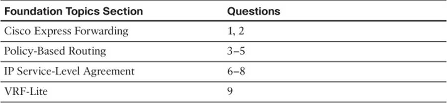
Table 11-1 “Do I Know This Already?” Foundation Topics Section-to-Question Mapping
1. Identify the architectural components of Cisco Express Forwarding (CEF). (Choose two.)
a. Routing Information Base (RIB)
b. Adjacency Table
c. Forwarding Information Base (FIB)
d. ARP Cache
2. What command can be used to globally enable CEF on a router?
a. ip flow egress
b. ip route-cache cef
c. no ip route-cache
d. ip cef
3. Policy-Based Routing (PBR) has been enabled on Router R1’s Fa 0/0 interface. Which of the following are true regarding how PBR works? (Choose two.)
a. Packets entering Fa 0/0 will be compared based on the PBR route map.
b. Packets exiting Fa 0/0 will be compared based on the PBR route map.
c. Cisco IOS ignores the PBR forwarding directions when a packet matches a route map deny clause.
d. Cisco IOS ignores the PBR forwarding directions when a packet matches a route map permit clause.
4. Examine the following configuration on Router R1. R1’s show ip route 172.16.4.1 command lists a route with outgoing interface S0/1/1. Host 172.16.3.3 uses Telnet to connect to host 172.16.4.1. What will Router R1 do with the packets generated by host 172.16.3.3 because of the Telnet session, assuming that the packets enter R1’s Fa0/0 interface? (Choose two.)
interface Fastethernet 0/0
ip address 172.16.1.1 255.255.255.0
ip policy route-map Q2
!
route-map Q2 permit
match ip address 101
set interface s0/0/1
!
access-list 101 permit tcp host 172.16.3.3 172.16.4.0 0.0.0.255
a. The packets will be forwarded out S0/0/1, or not at all.
b. The packets will be forwarded out S0/0/1 if it is up.
c. The packets will be forwarded out S0/1/1 if it is up.
d. The packets will be forwarded out S0/1/1 if it is up, or if it is not up, out S0/0/1.
e. The packets will be forwarded out S0/0/1 if it is up, or if it is not up, out S0/1/1.
5. The following output occurs on Router R2. Which of the following statements can be confirmed as true based on the output?
R2# show ip policy
Interface Route map
Fa0/0 RM1
Fa0/1 RM2
S0/0/0 RM3
a. R2 will forward all packets that enter Fa0/0 per the PBR configuration.
b. R2 will use route map RM2 when determining how to forward packets that exit interface Fa0/1.
c. R2 will consider using PBR for all packets exiting S0/0/0 per route map RM3.
d. R2 will consider using PBR for all packets entering S0/0/0 per route map RM3.
6. Which of the following are examples of traffic that can be created as part of an IP Service-Level Agreement operation? (Choose two.)
a. ICMP Echo
b. VoIP (RTP)
c. IPX
d. SNMP
7. The following configuration commands exist only in an implementation plan document. An engineer does a copy/paste of these commands into Router R1’s configuration. Which of the following answers is most accurate regarding the results?
ip sla 1
icmp-echo 1.1.1.1 source-ip 2.2.2.2
ip sla schedule 1 start-time now life forever
a. The SLA operation will be configured but will not start until additional commands are used.
b. The SLA operation is not completely configured, so it will not collect any data.
c. The SLA operation is complete and working, collecting data into the RTTMON MIB.
d. The SLA operation is complete and working but will not store the data in the RTTMON MIB without more configuration.
8. The following output occurs on Router R1. IP SLA operation 1 uses an ICMP echo operation type, with a default frequency of 60 seconds. The operation pings from address 1.1.1.1 to address 2.2.2.2. Which of the following answers is true regarding IP SLA and object tracking on R1?
R1# show track
Track 2
IP SLA 1 state
State is Up
3 changes, last change 00:00:03
Delay up 45 secs, down 55 secs
Latest operation return code: OK
Latest RTT (millisecs) 6
Tracked by:
STATIC-IP-ROUTING 0
a. The tracking return code fails immediately after the SLA operation results in an ICMP echo failure three times.
b. The tracking return code fails immediately after the SLA operation results in an ICMP echo failure one time.
c. After the tracking object fails, the tracking object moves back to an up state 45 seconds later in all cases.
d. After moving to a down state, the tracking object moves back to an OK state 45 seconds after the SLA operation moves to an OK state.
9. Which of the following is a benefit of Cisco EVN as compared to VRF-Lite?
a. Cisco EVN allows a single physical router to run multiple virtual router instances.
b. Cisco EVN allows two routers to be interconnected through an 802.1Q trunk, and traffic for different VRFs is sent over the trunk, using router subinterfaces.
c. Cisco EVN allows routes from one VRF to be selectively leaked to other VRFs.
d. Cisco EVN allows two routers to be interconnected through a VNET trunk, and traffic for different VRFs is sent over the trunk, without the need to configure router subinterfaces.
Foundation Topics
Cisco Express Forwarding
Much of the literature on router architecture divides router functions into three operational planes:
![]() Management plane: The management plane is concerned with the management of the device. For example, an administrator connecting to a router through a Secure Shell (SSH) connection through one of the router’s VTY lines would be a management plane operation.
Management plane: The management plane is concerned with the management of the device. For example, an administrator connecting to a router through a Secure Shell (SSH) connection through one of the router’s VTY lines would be a management plane operation.
![]() Control plane: The control plane is concerned with making packet-forwarding decisions. For example, routing protocol operation would be a control plane function.
Control plane: The control plane is concerned with making packet-forwarding decisions. For example, routing protocol operation would be a control plane function.
![]() Data plane: The data plane is concerned with the forwarding of data through a router. For example, end-user traffic traveling from a user’s PC to a web server on a different network would go across the data plane.
Data plane: The data plane is concerned with the forwarding of data through a router. For example, end-user traffic traveling from a user’s PC to a web server on a different network would go across the data plane.
Of these three planes, the two planes that most directly impact how quickly packets can flow through a router are the control plane and the data plane. Therefore, we will consider these two planes of operation and examine three different approaches that Cisco routers can take to forward packets arriving on an ingress interface and being sent out an appropriate egress interface, a process called packet switching.
Note
Many learners have a challenge with the term packet switching, because they are accustomed to switching being a Layer 2 operation, while routing is a Layer 3 operation. The key to understanding this term is to think of frame switching being a Layer 2 operation, while packet switching (the same thing as routing) is a Layer 3 operation.
In general, Cisco routers support the following three primary modes of packet switching:
![]() Process switching
Process switching
![]() Fast switching
Fast switching
![]() Cisco Express Forwarding (CEF)
Cisco Express Forwarding (CEF)
The following subsections discuss each of these approaches.
Operation of Process Switching
When a router routes a packet (that is, performs packet switching), the router removes the packet’s Layer 2 header, examines the Layer 3 addressing, and decides how to forward the packet. The Layer 2 header is then rewritten (which might involve changing the source and destination MAC addresses and computing a new cyclic redundancy check [CRC]), and the packet is forwarded out an appropriate interface. With process switching, as illustrated in Figure 11-1, a router’s CPU becomes directly involved with packet-switching decisions. As a result, the performance of a router configured for process switching can suffer significantly.
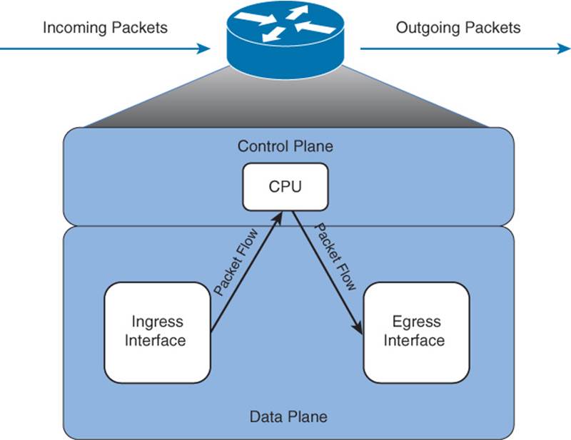
Figure 11-1 Data Flow with Process Switching
An interface can be configured for process switching by disabling fast switching on that interface. The interface configuration mode command used to disable fast switching is no ip route-cache.
Operation of Fast Switching
Fast switching uses a fast cache maintained in a router’s data plane. The fast cache contains information about how traffic from different data flows should be forwarded. As seen in Figure 11-2, the first packet in a data flow is process switched by a router’s CPU. After the router determines how to forward the first frame of a data flow, the forwarding information is stored in the fast cache. Subsequent packets in that same data flow are forwarded based on information in the fast cache, as opposed to being process switched. As a result, fast switching dramatically reduces a router’s CPU utilization, as compared to process switching.
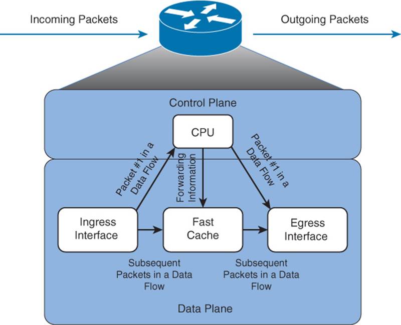
Figure 11-2 Data Flow with Fast Switching
Fast switching can be configured in interface configuration mode with the command ip route-cache.
Operation of Cisco Express Forwarding
Cisco Express Forwarding (CEF) maintains two tables in the data plane. Specifically, the Forwarding Information Base (FIB) maintains Layer 3 forwarding information, whereas the adjacency table maintains Layer 2 information for next hops listed in the FIB.
Using these tables, populated from a router’s IP routing table and ARP cache, CEF can efficiently make forwarding decisions. Unlike fast switching, CEF does not require the first packet of a data flow to be process switched. Rather, an entire data flow can be forwarded at the data plane, as seen in Figure 11-3.
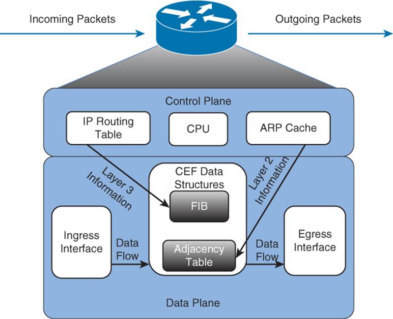
Figure 11-3 Data Flow with Cisco Express Forwarding
On many router platforms, CEF is enabled by default. If it is not, you can globally enable it with the ip cef command. Alternately, if CEF is enabled globally but is not enabled on a specific interface, you can enable it on that interface with the interface configuration mode command ip route-cache cef.
Table 11-2 lists and describes the configuration and verification commands for CEF.

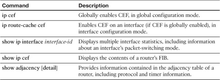
Table 11-2 CEF Configuration and Verification Commands
To illustrate the configuration and operation of CEF, the remainder of this section presents a series of CEF configuration and verification examples. Each of these examples is based on the topology shown in Figure 11-4. The routers in this topology have already been configured to exchange routes through Enhanced Interior Gateway Routing Protocol (EIGRP).
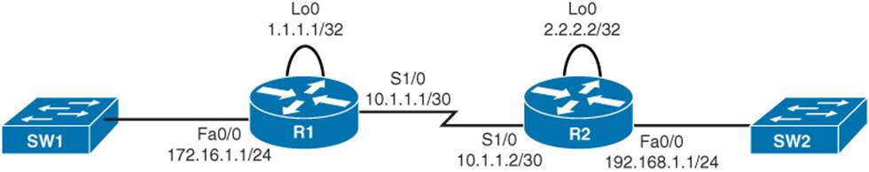
Figure 11-4 Sample Topology Configured with CEF
Router R1 in Figure 11-4 has CEF enabled globally; however, CEF is not enabled on interface Fa 0/0. Example 11-1 shows how to enable CEF on an interface if CEF is already enabled globally.
Example 11-1 Enable CEF on Router R1’s Fa 0/0 Interface
R1# show ip int fa 0/0
FastEthernet0/0 is up, line protocol is up
Internet address is 172.16.1.1/24
Broadcast address is 255.255.255.255
Address determined by non-volatile memory
MTU is 1500 bytes
Helper address is not set
Directed broadcast forwarding is disabled
Multicast reserved groups joined: 224.0.0.10
Outgoing access list is not set
Inbound access list is not set
Proxy ARP is enabled
Local Proxy ARP is disabled
Security level is default
Split horizon is enabled
ICMP redirects are always sent
ICMP unreachables are always sent
ICMP mask replies are never sent
IP fast switching is enabled
IP Flow switching is disabled
IP CEF switching is disabled
... OUTPUT OMITTED ...
R1# conf term
R1(config)# int fa 0/0
R1(config-if)# ip route-cache cef
R1(config-if)# end
R1# show ip int fa 0/0
FastEthernet0/0 is up, line protocol is up
Internet address is 172.16.1.1/24
Broadcast address is 255.255.255.255
Address determined by non-volatile memory
MTU is 1500 bytes
Helper address is not set
Directed broadcast forwarding is disabled
Multicast reserved groups joined: 224.0.0.10
Outgoing access list is not set
Inbound access list is not set
Proxy ARP is enabled
Local Proxy ARP is disabled
Security level is default
Split horizon is enabled
ICMP redirects are always sent
ICMP unreachables are always sent
ICMP mask replies are never sent
IP fast switching is enabled
IP Flow switching is disabled
IP CEF switching is enabled
... OUTPUT OMITTED ...
Router R2 in Figure 11-4 has CEF disabled globally. Example 11-2 shows how to globally enable CEF.
Example 11-2 Enable CEF on Router R2
R2# show ip int fa 0/0
FastEthernet0/0 is up, line protocol is up
Internet address is 192.168.1.1/24
Broadcast address is 255.255.255.255
Address determined by non-volatile memory
MTU is 1500 bytes
Helper address is not set
Directed broadcast forwarding is disabled
Multicast reserved groups joined: 224.0.0.10
Outgoing access list is not set
Inbound access list is not set
Proxy ARP is enabled
Local Proxy ARP is disabled
Security level is default
Split horizon is enabled
ICMP redirects are always sent
ICMP unreachables are always sent
ICMP mask replies are never sent
IP fast switching is disabled
IP Flow switching is disabled
IP CEF switching is disabled
... OUTPUT OMITTED ...
R2# conf term
R2(config)# ip cef
R2(config)# end
R2# show ip int fa 0/0
FastEthernet0/0 is up, line protocol is up
Internet address is 192.168.1.1/24
Broadcast address is 255.255.255.255
Address determined by non-volatile memory
MTU is 1500 bytes
Helper address is not set
Directed broadcast forwarding is disabled
Multicast reserved groups joined: 224.0.0.10
Outgoing access list is not set
Inbound access list is not set
Proxy ARP is enabled
Local Proxy ARP is disabled
Security level is default
Split horizon is enabled
ICMP redirects are always sent
ICMP unreachables are always sent
ICMP mask replies are never sent
IP fast switching is enabled
IP Flow switching is disabled
IP CEF switching is enabled
... OUTPUT OMITTED ...
Example 11-3 shows the output of the show ip cef and show adjacency detail commands issued on Router R1.
Example 11-3 Output from the show ip cef and show adjacency detail Commands
R1# show ip cef
Prefix Next Hop Interface
0.0.0.0/0 no route
0.0.0.0/8 drop
0.0.0.0/32 receive
1.1.1.1/32 receive Loopback0
2.2.2.2/32 10.1.1.2 Serial1/0
10.1.1.0/30 attached Serial1/0
10.1.1.0/32 receive Serial1/0
10.1.1.1/32 receive Serial1/0
10.1.1.3/32 receive Serial1/0
127.0.0.0/8 drop
172.16.1.0/24 attached FastEthernet0/0
172.16.1.0/32 receive FastEthernet0/0
172.16.1.1/32 receive FastEthernet0/0
172.16.1.255/32 receive FastEthernet0/0
192.168.1.0/24 10.1.1.2 Serial1/0
224.0.0.0/4 drop
224.0.0.0/24 receive
240.0.0.0/4 drop
255.255.255.255/32 receive
R1# show adjacency detail
Protocol Interface Address
IP Serial1/0 point2point(11)
0 packets, 0 bytes
epoch 0
sourced in sev-epoch 1
Encap length 4
0F000800
P2P-ADJ
Output from the show ip cef command, as seen in Example 11-3, contains the contents of the FIB for Router R1. Note that if the next hop of a network prefix is set to attached, the entry represents a network to which the router is directly attached. However, if the next hop of a network prefix is set to receive, the entry represents an IP address on one of the router’s interfaces.
For example, the network prefix 10.1.1.0/30, with a next hop of attached, is a network (as indicated by the 30-bit subnet mask) directly attached to Router R1’s Serial 1/0 interface. However, the network prefix of 10.1.1.1/32 with a next hop of receive is a specific IP address (as indicated by the 32-bit subnet mask). Note that the all-0s host addresses for directly attached networks (for example, 10.1.1.0/30) and the all-1s host addresses for directly attached networks (for example, 172.16.1.255/32) also show up as receive entries.
Output from the show adjacency detail command displays information about how to reach a specific adjacency shown in the FIB. For example, Example 11-3 indicates that network 192.168.1.0 /24 is reachable by going out of interface Serial 1/0. The adjacency table also shows interface Serial 1/0 uses a point-to-point connection. Therefore, the adjacent router is on the other side of the point-to-point link. If an interface in the adjacency table is an Ethernet interface, source and destination MAC address information is contained in the entry for the interface.
Policy-Based Routing
When a packet arrives at the incoming interface of a router, the router’s data plane processing logic takes several steps to process the packet. The incoming packet actually arrives encapsulated inside a data link layer frame, so the router must check the incoming frame’s Frame Check Sequence (FCS) and discard the frame if errors occurred in transmission. If the FCS check passes, the router discards the incoming frame’s data-link header and trailer, leaving the Layer 3 packet. Finally, the router does the equivalent of comparing the destination IP address of the packet with the IP routing table, matching the longest-prefix route that matches the destination IP address.
Policy-Based Routing (PBR) overrides a router’s natural destination-based forwarding logic. PBR intercepts the packet after deencapsulation on the incoming interface, before the router performs the CEF table lookup. PBR then chooses how to forward the packet using criteria other than the usual matching of the packet’s destination address with the CEF table.
PBR chooses how to forward the packet by using matching logic defined through a route map, which in turn typically refers to an IP access control list (ACL). That same route map also defines the forwarding instructions—the next-hop IP address or outgoing interface—for packets matched by the route map. Figure 11-5 shows the general concept, with PBR on interface Fa0/0 overriding the usual routing logic, forwarding packets out three different outgoing interfaces.
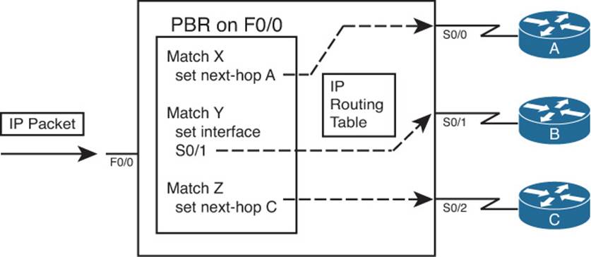
Figure 11-5 PBR Concepts
To perform the actions shown in Figure 11-5, the engineer configures two general steps:
Step 1. Create a route map with the logic to match packets, and choose the route, as shown on the left side of the figure.
Step 2. Enable the route map for use with PBR, on an interface, for packets entering the interface.
The rest of this section focuses on the configuration and verification of PBR.
Matching the Packet and Setting the Route
To match packets with a route map enabled for PBR, you use the familiar route-map match command. However, you have two match command options to use:
![]() match ip address
match ip address
![]() match length min max
match length min max
The match ip address command can reference standard and extended ACLs. Any item matchable by an ACL can be matched in the route map. The match length command allows you to specify a range of lengths, in bytes.
When a route map clause (with a permit action) matches a packet, the set command defines the action to take regarding how to forward the packet. The four set command options define either the outgoing interface or the next-hop IP address, just like routes in the IP routing table. Table 11-3lists the options, with some explanations.
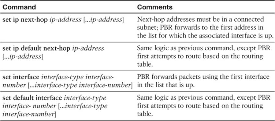
Table 11-3 Choosing Routes Using the PBR set Command
Note that two of the commands allow the definition of a next-hop router, and two allow the definition of an outgoing interface. The other difference in the commands relates to whether the command includes the default keyword. The section “How the default Keyword Impacts PBR Logic Ordering,” later in this chapter, describes the meaning of the default keyword.
After the route map has been configured with all the clauses to match packets and to set an outgoing interface or next-hop address, the only remaining step requires the ip policy route-map name command to enable PBR for packets entering an interface.
PBR Configuration Example
To tie the concepts together, Figure 11-6 shows a sample internetwork to use in a PBR example. In this case, EIGRP on R1 chooses the upper route to reach the subnets on the right, because of the higher bandwidth on the upper link (T1) as compared with the lower link (64 kbps).
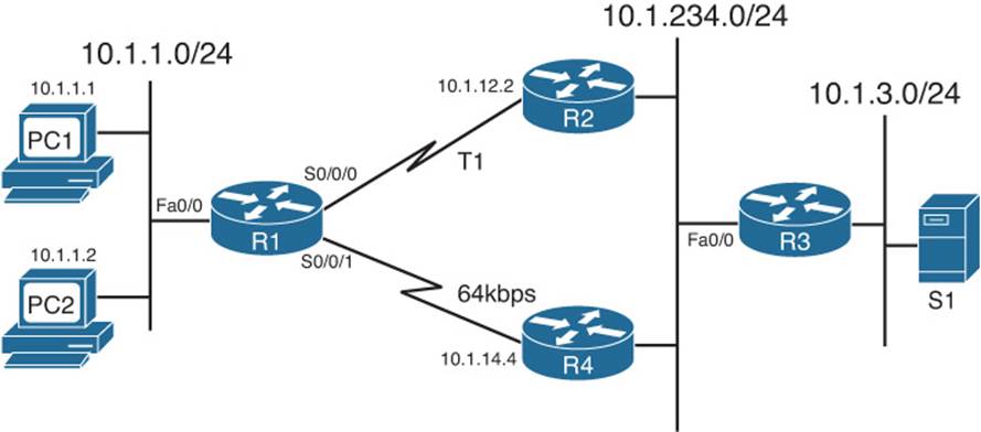
Figure 11-6 Network Used in PBR Example
For this example, the PBR configuration matches packets sent from PC2 on the left to server S1 in subnet 10.1.3.0/24 on the right. PBR on R1 routes these packets out S0/0/1 to R4. These packets will be routed over the lower path—out R1’s S0/0/1 to R4—instead of through the current through R2, as listed in R1’s IP routing table. The PBR configuration on Router R1 is shown in Example 11-4.
Example 11-4 R1 PBR Configuration
interface Fastethernet 0/0
ip address 10.1.1.9 255.255.255.0
ip policy route-map PC2-over-low-route
!
route-map PC2-over-low-route permit
match ip address 101
set ip next-hop 10.1.14.4
!
access-list 101 permit ip host 10.1.1.2 10.1.3.0 0.0.0.255
The configuration enables PBR with Fa0/0’s ip policy route-map PC2-over-low-route command. The referenced route map matches packets that match ACL 101; ACL 101 matches packets from PC2 only, going to subnet 10.1.3.0/24. The route-map clause uses a permit action, which tells Cisco IOS to indeed apply PBR logic to these matched packets. (Had the route-map command listed a deny action, Cisco IOS would simply route the packet as normal—it would not filter the packet.) Finally, for packets matched with a permit action, the router forwards the packets based on the set ip next-hop 10.1.14.4 command, which tells R1 to forward the packet to R4 next.
Note that for each packet entering Fa0/0, PBR either matches a packet with a route map permit clause or matches a packet with a route map deny clause. All route maps have an implicit deny clause at the end that matches all packets not already matched by the route map. PBR processes packets that match a permit clause using the defined set command. For packets matched by a deny clause, PBR lets the packet go through to the normal IP routing process.
To verify the results of the policy routing, Example 11-5 shows two traceroute commands: one from PC1 and one from PC2. Each shows the different paths. (Note that the output actually comes from a couple of routers configured to act as hosts PC1 and PC2 for this example.)
Example 11-5 Confirming PBR Results Using traceroute
! First, from PC1 (actually, a router acting as PC1):
PC1# trace 10.1.3.99
Type escape sequence to abort.
Tracing the route to 10.1.3.99
1 10.1.1.9 4 msec 0 msec 4 msec
2 10.1.12.2 0 msec 4 msec 4 msec
3 10.1.234.3 0 msec 4 msec 4 msec
4 10.1.3.99 0 msec * 0 msec
! Next, from PC2
PC2# trace 10.1.3.99
Type escape sequence to abort.
Tracing the route to 10.1.3.99
1 10.1.1.9 4 msec 0 msec 4 msec
2 10.1.14.4 8 msec 4 msec 8 msec
3 10.1.234.3 8 msec 8 msec 4 msec
4 10.1.3.99 4 msec * 4 msec
The output differs only in the second router in the end-to-end path—R2’s 10.1.12.2 address as seen for PC1’s packet and 10.1.14.4 as seen for PC2’s packet.
The verification commands on the router doing the PBR function list relatively sparse information. The show ip policy command just shows the interfaces on which PBR is enabled and the route map used. The show route-map command shows overall statistics for the number of packets matching the route map for PBR purposes. The only way to verify the types of packets that are policy routed is to use the debug ip policy command, which can produce excessive overhead on production routers, given its multiple lines of output per packet, or to use traceroute. Example 11-6lists the output of the show and debug commands on Router R1, with the debug output being for a single policy-routed packet.
Example 11-6 Verifying PBR on Router R1
R1# show ip policy
Interface Route map
Fa0/0 PC2-over-low-route
R1# show route-map
route-map PC2-over-low-route, permit, sequence 10
Match clauses:
ip address (access-lists): 101
Set clauses:
ip next-hop 10.1.14.4
Policy routing matches: 12 packets, 720 bytes
R1# debug ip policy
*Sep 14 16:57:51.675: IP: s=10.1.1.2 (FastEthernet0/0), d=10.1.3.99, len 28,
policy match
*Sep 14 16:57:51.675: IP: route map PC2-over-low-route, item 10, permit
*Sep 14 16:57:51.675: IP: s=10.1.1.2 (FastEthernet0/0), d=10.1.3.99 (Serial0/0/1),
len 28, policy routed
*Sep 14 16:57:51.675: IP: FastEthernet0/0 to Serial0/0/1 10.1.14.4
How the default Keyword Impacts PBR Logic Ordering
The example in the previous section showed a set command that did not use the default keyword. However, the inclusion or omission of this keyword significantly impacts how PBR works. This parameter in effect tells Cisco IOS whether to apply PBR logic before trying to use normal destination-based routing, or whether to first try to use the normal destination-based routing, relying on PBR’s logic only if the destination-based routing logic fails to match a nondefault route.
First, consider the case in which the set command omits the default parameter. When Cisco IOS matches the associated PBR route map permit clause, Cisco IOS applies the PBR logic first. If the set command identifies an outgoing interface that is up, or a next-hop router that is reachable, Cisco IOS uses the PBR-defined route. However, if the PBR route (as defined in the set command) is not working—because the outgoing interface is down or the next hop is unreachable using a connected route—Cisco IOS next tries to route the packet using the normal destination-based IP routing process.
Next, consider the case in which the set command includes the default parameter. When Cisco IOS matches the associated PBR route map permit clause, Cisco IOS applies the normal destination-based routing logic first, with one small exception: It ignores any default routes. Therefore, the router first tries to route the packet as normal, but if no nondefault route matches the packet’s destination address, the router forwards the packet as directed in the set command.
For example, for the configuration shown in Example 11-4, by changing the set command to set ip default next-hop 10.1.14.4, R1 would have first looked for (and found) a working route through R2, and forwarded packets sent by PC2 over the link to R2. Summarizing:
![]() Omitting the default parameter gives you logic like this: “Try PBR first, and if PBR’s route does not work, try to route as usual.”
Omitting the default parameter gives you logic like this: “Try PBR first, and if PBR’s route does not work, try to route as usual.”
![]() Including the default parameter gives you logic like this: “Try to route as usual while ignoring any default routes, but if normal routing fails, use PBR.”
Including the default parameter gives you logic like this: “Try to route as usual while ignoring any default routes, but if normal routing fails, use PBR.”
Additional PBR Functions
Primarily, PBR routes packets received on an interface, but using logic other than matching the destination IP address and the CEF table. This section briefly examines three additional PBR functions.
Applying PBR to Locally Created Packets
In some cases, it might be useful to use PBR to process packets generated by the router itself. However, PBR normally processes packets that enter the interface(s) on which the ip policy route-map command has been configured, and packets generated by the router itself do not actually enter the router through some interface. To make Cisco IOS process locally created packets using PBR logic, configure the ip local policy route-map name global command, referring to the PBR route map at the end of the command.
The section “Configuring and Verifying IP SLA,” later in this chapter, shows an example use of this command. IP SLA causes a router to create packets, so applying PBR to such packets can influence the path taken by the packets.
Setting IP Precedence
Quality of service (QoS) refers to the entire process of how a network infrastructure can choose to apply different levels of service to different packets. For example, a router might need to keep delay and jitter (delay variation) low for VoIP and Video over IP packets, because these interactive voice and video calls only work well when the delay and jitter are held very low. As a result, the router might let VoIP packets bypass a long queue of data packets waiting to exit an interface, giving the voice packet better (lower) delay and jitter.
Most QoS designs mark each packet with a different value inside the IP header, for the purpose of identifying groups of packets—a service class—that should get a particular QoS treatment. For example, all VoIP packets could be marked with a particular value so that the router can then find those marked bits, know that the packets are VoIP packets because of that marking, and apply QoS accordingly.
Although the most commonly used QoS marking tool today is Class-Based Marking, in the past, PBR was one of the few tools that could be used for this important QoS function of marking packets. PBR still supports marking. However, most modern QoS designs ignore PBR’s marking capabilities.
Before discussing PBR’s marking features, a little background about the historical view of the IP header’s type of service (ToS) byte is needed. The IP header originally defined a ToS byte whose individual bits have been defined in a couple of ways over the years. One such definition used the three leftmost bits in the ToS byte as a 3-bit IP Precedence (IPP) field, which could be used for generic QoS marking, with higher values generally implying a better QoS treatment. Back in the 1990s, the ToS byte was redefined as the Differentiated Services (DS) byte, with the six leftmost bits defined as the Differentiated Service Code Point (DSCP) marking. Most QoS implementations today revolve around setting the DSCP value.
PBR supports setting the older QoS marking fields—the IP Precedence (IPP) and the entire ToS byte—using the commands set ip precedence value and set ip tos value, respectively, in a route map. To configure packet marking, configure PBR as normal, but add a set command that defines the field to be marked and the value.
PBR with IP SLA
Besides matching a packet’s length, or matching a packet with an ACL, PBR can also react to some dynamic measurements of the health of an IP network. To do so, PBR relies on the IP Service-Level Agreement (IP SLA) tool. In short, if the IP SLA tool measures the network’s current performance, and the performance does not meet the defined threshold, PBR chooses to not use a particular route. The last major section of this chapter discusses IP SLA, with the section “Configuring and Verifying IP SLA” demonstrating how PBR works with IP SLA.
IP Service-Level Agreement
The Cisco IOS IP Service-Level Agreement (IP SLA) feature measures the ongoing behavior of the network. The measurement can be as simple as using the equivalent of a ping to determine whether an IP address responds, or as sophisticated as measuring the jitter (delay variation) of VoIP packets that flow over a particular path. To use IP SLA, an engineer configures IP SLA operations on various routers, and the routers will then send packets, receive responses, and gather data about whether a response was received, and the specific characteristics of the results, such as delay and jitter measurements.
IP SLA primarily acts as a tool to test and gather data about a network. Network management tools can then collect that data and report whether the network reached SLAs for the network. Many network management tools support the ability to configure IP SLA from the management tools’ graphical interfaces. When configured, the routers gather the results of the operations, storing the statistics in the CISCO-RTTMON-MIB. Management applications can later gather the statistics from this management information base (MIB) on various routers and report on whether the business SLAs were met based on the gathered statistics.
Why bother with a pure network management feature in this book focused on IP routing? Well, you can configure static routes and PBR to use IP SLA operations, such that if an operation shows a failure of a particular measurement or a reduced performance of the measurement below a configured threshold, the router stops using either the static route or PBR logic. This combination of features provides a means to control when the static and PBR paths are used and when they are ignored.
This section begins with a discussion of IP SLA as an end to itself. Following that, the topic of SLA object tracking is added, along with how to configure static routes and PBR to track IP SLA operations, so that Cisco IOS knows when to use, and when to ignore, these routes.
Understanding IP SLA Concepts
IP SLA uses the concept of an operation. Each operation defines a type of packet that the router will generate, the destination and source address, and other characteristics of the packet. The configuration includes settings about the time of day when the router should be sending the packets in a particular operation, the types of statistics that should be gathered, and how often the router should send the packets. Also, you can configure a router with multiple operations of different types.
For example, a single IP SLA operation could define the following:
![]() Use Internet Control Message Protocol (ICMP) echo packets.
Use Internet Control Message Protocol (ICMP) echo packets.
![]() Measure the end-to-end round-trip response time (ICMP echo).
Measure the end-to-end round-trip response time (ICMP echo).
![]() Send the packets every 5 minutes, all day long.
Send the packets every 5 minutes, all day long.
Note
For those of you who have been around Cisco IOS for a while, the function of IP SLA might sound familiar. Cisco IP SLA has origins in earlier Cisco IOS features, including the Response Time Reporter (RTR) feature. The RTR feature is configured with the rtr command and uses the term probe to refer to what IP SLA refers to as an operation.
All the SLA operations rely on the router sending packets and some other device sending packets back. Figure 11-7 shows the general idea and provides a good backdrop to discuss some related issues.
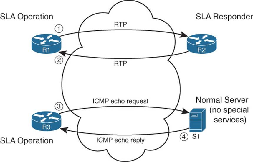
Figure 11-7 Sending and Receiving Packets with IP SLA
An IP SLA operation can cause the router to send packets to any IP address, whether on a router or a host. When sending to a host, as seen in the bottom part of the figure, the host does not need any special software or configuration—instead, the host just acts as normal. That means that if an SLA operation sends packets to a host, the router can only use operation types that send packets that the host understands. For example, the router could use ICMP echo requests (as seen in Steps 3 and 4), TCP connection requests, or even HTTP GET requests to a web server, because the server should try to respond to these requests.
The operation can also send packets to another router, which gives IP SLA a wider range of possible operation types. If the operation sends packets to which the remote router would normally respond, like ICMP echo requests, the other router needs no special configuration. However, IP SLA supports the concept of the IP SLA responder, as noted in Figure 11-7 for R2. By configuring R2 as an IP SLA responder, it responds to packets that a router would not normally respond to, giving the network engineer a way to monitor network behavior without having to place devices around the network just to test the network.
For example, the operation could send Real-time Transport Protocol (RTP) packets—packets that have the same characteristics as VoIP packets—as shown in Figure 11-7 as Step 1. Then the IP SLA responder function on R2 can reply as if a voice call exists between the two routers, as shown in Step 2 of that figure.
A wide range of IP SLA operations exist. The following list summarizes the majority of the available operation types, just for perspective:
![]() ICMP (echo, jitter)
ICMP (echo, jitter)
![]() RTP (VoIP)
RTP (VoIP)
![]() TCP connection (establishes TCP connections)
TCP connection (establishes TCP connections)
![]() UDP (echo, jitter)
UDP (echo, jitter)
![]() DNS
DNS
![]() DHCP
DHCP
![]() HTTP
HTTP
![]() FTP
FTP
Configuring and Verifying IP SLA
This book describes IP SLA configuration in enough depth to get a sense for how it can be used to influence static routes and PBR. To that end, this section examines the use of an ICMP echo operation, which requires configuration only on one router, with no IP SLA responder. The remote host, router, or other device replies to the ICMP echo requests just like any other ICMP echo requests.
The general steps to configure an ICMP-based IP SLA operation are as follows:
Step 1. Create the IP SLA operation and assign it an integer operation number, using the ip sla sla-ops-number global configuration command.
Step 2. Define the operation type and the parameters for that operation type. For ICMP echo, you define the destination IP address or host name, and optionally, the source IP address or host name, using the icmp-echo {destination-ip-address | destination-hostname} [source-ip {ip-address | hostname} | source-interface interface-name] SLA operation subcommand.
Step 3. (Optional) Define a (nondefault) frequency at which the operation should send the packets, in seconds, using the frequency seconds IP SLA subcommand.
Step 4. Schedule when the SLA will run, using the ip sla schedule sla-ops-number [life {forever | seconds}] [start-time {hh:mm[:ss] [month day | day month] | pending | now | after hh:mm:ss}] [ageout seconds] [recurring] global command.
Example 11-7 shows the process of configuring an ICMP echo operation on Router R1 from Figure 11-6. The purpose of the operation is to test the PBR route through R4. In this case, the operation will be configured as shown in Figure 11-8, with the following criteria:
![]() Send ICMP echo requests to server S1 (10.1.3.99).
Send ICMP echo requests to server S1 (10.1.3.99).
![]() Use source address 10.1.1.9 (R1’s F0/0 IP address).
Use source address 10.1.1.9 (R1’s F0/0 IP address).
![]() Send these packets every 60 seconds.
Send these packets every 60 seconds.
![]() Start the operation immediately, and run it forever.
Start the operation immediately, and run it forever.
![]() Enable PBR for locally generated packets, matching the IP SLA operation with the PBR configuration so that the SLA operation’s packets flow over the lower route.
Enable PBR for locally generated packets, matching the IP SLA operation with the PBR configuration so that the SLA operation’s packets flow over the lower route.
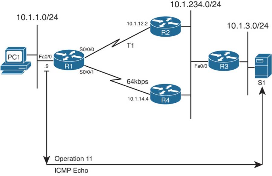
Figure 11-8 Concept of IP SLA Operation on R1
Example 11-7 Configuring an ICMP Echo Operation on Router R1
R1# conf t
Enter configuration commands, one per line. End with CNTL/Z.
R1(config)# ip sla 11
R1(config-ip-sla)# icmp?
icmp-echo icmp-jitter
R1(config-ip-sla)# icmp-echo 10.1.3.99 source-ip 10.1.1.9
R1(config-ip-sla)# frequency 60
R1(config-ip-sla)# exit
R1(config)# ip sla schedule 11 start-time now life forever
! Changes to the PBR configuration below
R1(config)# access-list 101 permit ip host 10.1.1.9 host 10.1.3.99
R1(config)# ip local policy route-map PC2-over-low-route
R1(config)# end
First, focus on the pure IP SLA configuration, located from the beginning of the example through command ip sla schedule. The configuration creates IP SLA operation 11. The parameters on the icmp-echo command act as if you used an extended ping from the command line, specifying both the source and destination IP address. The last command directly relates to IP SLA. The ip sla schedule command enables the operation now, and runs the operation until the network engineer takes some action to disable it, in some cases by removing the operation with the no ip sla sla-ops-number command.
The last two commands in the example show a change to the earlier PBR configuration so that the SLA operation’s packets flow over the lower route. The ip local policy PC2-over-low-route global configuration command tells R1 to process packets generated by R1, including the IP SLA operation packets, using PBR. The addition of the access-list 101 command to the configuration shown earlier in Example 11-4 makes the route map match the source and destination address of the SLA operation. That former route map’s set command sent the packets over the link to R4.
IP SLA supports a couple of particularly useful verification commands: show ip sla configuration and show ip sla statistics. The first command confirms all the configuration settings for the operation, and the second lists the current statistics for the operation. Example 11-8 shows examples of each on R1, after the configuration shown in Example 11-7.
Example 11-8 Verification of an IP SLA Operation
R1# show ip sla configuration
IP SLAs Infrastructure Engine-II
Entry number: 11
Owner:
Tag:
Type of operation to perform: echo
Target address/Source address: 10.1.3.99/10.1.1.9
Type Of Service parameter: 0x0
Request size (ARR data portion): 28
Operation timeout (milliseconds): 5000
Verify data: No
Vrf Name:
Schedule:
Operation frequency (seconds): 60 (not considered if randomly scheduled)
Next Scheduled Start Time: Start Time already passed
Group Scheduled : FALSE
Randomly Scheduled : FALSE
Life (seconds): Forever
Entry Ageout (seconds): never
Recurring (Starting Everyday): FALSE
Status of entry (SNMP RowStatus): Active
Threshold (milliseconds): 5000 (not considered if react RTT is configured)
Distribution Statistics:
Number of statistic hours kept: 2
Number of statistic distribution buckets kept: 1
Statistic distribution interval (milliseconds): 20
History Statistics:
Number of history Lives kept: 0
Number of history Buckets kept: 15
History Filter Type: None
Enhanced History:
R1# show ip sla statistics 11
IPSLAs Latest Operation Statistics
IPSLA operation id: 11
Latest RTT: 8 milliseconds
Latest operation start time: *19:58:08.395 UTC Mon Sep 14 2009
Latest operation return code: OK
Number of successes: 22
Number of failures: 0
Operation time to live: Forever
The highlighted lines in the output of the show ip sla configuration command correspond to the values explicitly configured in Example 11-7. The more interesting output exists in the output of the show ip sla statistics 11 command, which lists the statistics only for operation 11. In this case, 22 intervals have passed, showing 22 ICMP echo requests as successful with no failures. The output also lists the latest round-trip time (RTT). Finally, it lists the return code of the most recent operation (OK in this case)—a key value used by SLA tracking.
Tracking SLA Operations to Influence Routing
As previously mentioned, you can configure both static routes and PBR to be used only when an SLA operation remains successful. The configuration to achieve this logic requires the configuration of a tracking object and cross-references between the static route, PBR, and IP SLA, as shown in Figure 11-9.
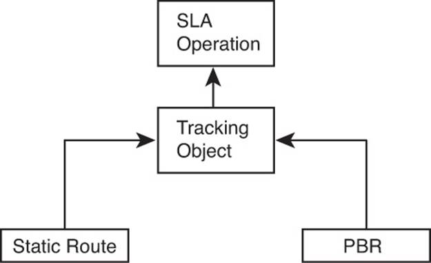
Figure 11-9 Configuration Relationships for Path Control Using IP SLA
The tracking object looks at the IP SLA operation’s most recent return code to then determine the tracking state as either “up” or “down.” Depending on the type of SLA operation, the return code can be a simple toggle, with “OK” meaning that the last operation worked. The tracking object would then result in an “up” state if the SLA operation resulted in an “OK” return code. Other SLA operations that define thresholds have more possible return codes. The tracking operation results in an “up” state if the IP SLA operation is within the configured threshold.
One of the main reasons that Cisco IOS requires the use of this tracking object is to prevent flapping routes. Route flapping occurs when a router adds a route to its routing table then quickly removes it, conditions change causing the route to be added back to the table again, and so on. If a static route tracked an IP SLA object directly, the SLA object’s return code could change each time the operation ran, causing a route flap. The tracking object concept provides the ability to set a delay of how soon after a tracking state change the tracking object should change state. This feature gives the engineer a tool to control route flaps.
This section shows how to configure a tracking object for use with both a static route and with PBR.
Configuring a Static Route to Track an IP SLA Operation
To configure a static route to track an IP SLA, you need to configure the tracking object and then configure the static route with the track keyword. To do so, use these steps:
Step 1. Use the track object-number ip sla sla-ops-number [state | reachability] global command.
Step 2. (Optional) Configure the delay to regulate flapping of the tracking state by using the delay {down seconds | up seconds} command in tracking configuration mode.
Step 3. Configure the static route with the ip route destination mask {interface | next-hop} track object-number command in global configuration mode.
Example 11-9 shows the configuration of tracking object 2, using the same design shown in Figures 11-6 and 11-8. In this case, the configuration adds a static route for subnet 10.1.234.0/24, the LAN subnet to which R2, R3, and R4 all connect. EIGRP chooses a route over R1’s S0/0/0 interface as its best route, but this static route uses S0/0/1 as the outgoing interface.
Example 11-9 Configuring a Static Route with Tracking IP SLA
R1# conf t
Enter configuration commands, one per line. End with CNTL/Z.
R1(config)# track 2 ip sla 11 state
R1(config-track)# delay up 90 down 90
R1(config-track)# exit
R1(config)# ip route 10.1.234.0 255.255.255.0 s0/0/1 track 2
R1(config)# end
The configuration begins with the creation of the tracking object number 2. As with IP SLA operation numbers, the number itself is unimportant, other than that the ip route command refers to this same number with the track 2 option at the end of the command. The tracking object’s delay settings have been made at 90 seconds.
The show track command lists the tracking object’s configuration plus many other details. It lists the current tracking state, the time in this state, the number of state transitions, and the other entities that track the object (in this case, a static route).
Example 11-10 shows what happens when the IP SLA operation fails, causing the static route to be removed. The example starts with the configuration shown in Example 11-9, along with the SLA operation 11 as configured in Example 11-7. The following list details the current operation and what happens sequentially in the example:
Step 1. Before the text seen in Example 11-10, the current IP SLA operation already sends packets using PBR, over R1’s link to R4, using source IP address 10.1.1.9 and destination 10.1.3.99 (server S1).
Step 2. At the beginning of the next example, because the IP SLA operation is working, the static route is in R1’s IP routing table.
Step 3. An ACL is configured on R4 (not shown) so that the IP SLA operation fails.
Step 4. A few minutes later, R1 issues a log message stating that the tracking object changed state from up to down.
Step 5. The example ends with several commands that confirm the change in state for the tracking object, and confirmation that R1 now uses the EIGRP-learned route through R2.
Note
This example uses the show ip route ... longer-prefixes command, because this command lists only the route for 10.1.234.0/24, which is the route that fails over in the example.
Example 11-10 Verifying Tracking of Static Routes
! Next – Step 2
R1# show ip route 10.1.234.0 255.255.255.0 longer-prefixes
! Legend omitted for brevity
10.0.0.0/8 is variably subnetted, 7 subnets, 2 masks
S 10.1.234.0/24 is directly connected, Serial0/0/1
R1# show track
Track 2
IP SLA 11 state
State is Up
1 change, last change 01:24:14
Delay up 90 secs, down 90 secs
Latest operation return code: OK
Latest RTT (millisecs) 7
Tracked by:
STATIC-IP-ROUTING 0
! Next, Step 3
! Not shown – SLA Operations packets are now filtered by an ACL on R4
! Sometime later...
!
! Next – Step 4
R1#
*Sep 14 22:55:43.362: %TRACKING-5-STATE: 2 ip sla 11 state Up->Down
! Final Step – Step 5
R1# show track
Track 2
IP SLA 11 state
State is Down
2 changes, last change 00:00:15
Delay up 90 secs, down 90 secs
Latest operation return code: No connection
Tracked by:
STATIC-IP-ROUTING 0
R1# show ip route 10.1.234.0 255.255.255.0 longer-prefixes
! Legend omitted for brevity
10.0.0.0/8 is variably subnetted, 7 subnets, 2 masks
D 10.1.234.0/24 [90/2172416] via 10.1.12.2, 00:00:25, Serial0/0/0
Configuring PBR to Track an IP SLA
To configure PBR to use object tracking, use a modified version of the set command in the route map. For example, the earlier PBR configuration used the following set command:
set ip next-hop 10.1.14.4
Instead, use the verify-availability keyword, as shown in this command:
set ip next-hop verify-availability 10.1.14.4 1 track 2
When the tracking object is up, PBR works as configured. When the tracking object is down, PBR acts as if the set command does not exist. That means that the router will still attempt to route the packet per the normal destination-based routing process.
The output of the related verification commands does not differ significantly when comparing the configuration of tracking for static routes versus PBR. The show track command lists “ROUTE-MAP” instead of “STATIC-IP-ROUTING,” but the details of the show track, show ip sla statistics, and object tracking log message seen in Example 11-10 remain the same.
VRF-Lite
Service providers often need to allow their customers’ traffic to pass through their cloud without one customer’s traffic (and corresponding routes) exposed to another customer. Similarly, enterprise networks might need to segregate various application types, such as keeping voice and video traffic separate from data. These are just a couple of scenarios that could benefit from the Cisco Virtual Routing and Forwarding (VRF) feature. VRF allows a single physical router to host multiple virtual routers, with those virtual routers logically isolated from one another, each with its own IP routing table.
Note
Some Cisco literature states that VRF is an acronym for Virtual Routing and Forwarding, while other Cisco literature states that VRF is an acronym for VPN Routing/Forwarding (because of its common use in Virtual Private Networks [VPN]). This book uses the more genericVirtual Routing and Forwarding definition.
Cisco Easy Virtual Network (EVN), as described in Chapter 1, “Characteristics of Routing Protocols,” is a newer approach to VRF configuration, as compared to VRF-Lite. With VRF-Lite, if you want to send traffic for multiple virtual networks (that is, multiple VRFs) between two routers, you need to create a subinterface for each VRF on each router. However, with Cisco EVN, you instead create a trunk (called a Virtual Network (VNET) trunk) between the routers. Then, traffic for multiple virtual networks can travel over that single trunk interface, which uses tags to identify the virtual networks to which packets belong.
Even though Cisco EVN can help reduce the amount of configuration required for a VRF solution, VRF-Lite configuration is still often used in VRF networks. This section covers the basics of setting up and verifying a VRF configuration, for VRFs using Open Shortest Path First (OSPF) as their interior gateway protocol (IGP).
VRF-Lite Configuration
Table 11-4 lists the steps to perform a basic VRF-Lite configuration for VRF instances running OSPF.
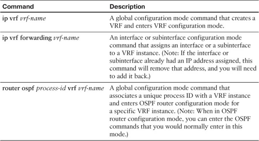
Table 11-4 Steps for a Basic OSPF VRF-Lite Configuration
Note
VRF-Lite has several other options, beyond the scope of this book. For example, you can allow VRF to selectively “leak” routes between VRF instances.
To illustrate a basic VRF-Lite configuration, consider Figure 11-10. A goal of the network topology shown is to isolate the voice, data, and video networks into separate VRF instances. Notice that the Fa 0/0 interface on the COMMON router is divided into three subinterfaces (Fa 0/0.2, Fa 0/0.3, and Fa 0/0.4). The COMMON router then connects to switch SW1 over an 802.1Q trunk. Switch SW1 then connects out to the VOICE, DATA, and VIDEO routers, where the switch port connecting to each router belongs to a different VLAN (that is, VOICE VLAN = 2, DATA VLAN = 3, VIDEO VLAN = 4).
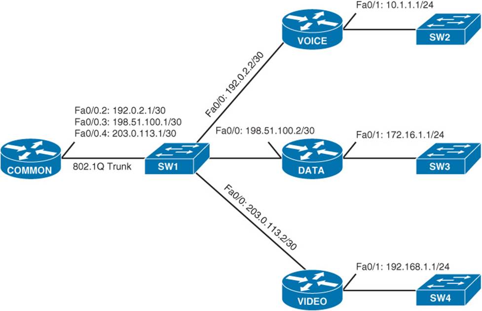
Figure 11-10 VRF-Lite Sample Topology
Example 11-11 illustrates the configuration of the three VRFs (VOICE, DATA, and VIDEO) shown in Figure 11-10.
Example 11-11 VRF-Lite Sample Configuration Using OSPF as the Routing Protocol
... OUTPUT OMITTED...
ip vrf VOICE
!
ip vrf DATA
!
ip vrf VIDEO
!
... OUTPUT OMITTED...
!
interface FastEthernet0/0
no ip address
!
interface FastEthernet0/0.2
encapsulation dot1Q 2
ip vrf forwarding VOICE
ip address 192.0.2.1 255.255.255.252
!
interface FastEthernet0/0.3
encapsulation dot1Q 3
ip vrf forwarding DATA
ip address 198.51.100.1 255.255.255.252
!
interface FastEthernet0/0.4
encapsulation dot1Q 4
ip vrf forwarding VIDEO
ip address 203.0.113.1 255.255.255.252
!
... OUTPUT OMITTED...
!
router ospf 1 vrf VOICE
network 0.0.0.0 255.255.255.255 area 0
!
router ospf 2 vrf DATA
network 0.0.0.0 255.255.255.255 area 0
!
router ospf 3 vrf VIDEO
network 0.0.0.0 255.255.255.255 area 0
... OUTPUT OMITTED...
In Example 11-11, notice that the ip vrf vrf-name command is used to create each of the VRFs. Then each subinterface is assigned to one of the VRFs, using the ip vrf forwarding vrf-name command. If the subinterface previously had an IP address, the ip vrf forwarding vrf-name command removes the address, and it has to be reentered.
This example used OSPF as the routing protocol for the different VRFs, and the router ospf process-id vrf vrf-name command was used to enter OSPF configuration mode for each VRF. Also, keep in mind that even though different VRFs can have overlapping network addresses (because the VRF’s IP routing tables are logically separated), the OSPF process ID needs to be unique for each VRF.
VRF Verification
The show ip vrf command, as demonstrated in Example 11-12, can be used to list a router’s VRFs, along with the interfaces assigned to each VRF.
Example 11-12 show ip vrf Output
COMMON# show ip vrf
Name Default RD Interfaces
DATA <not set> Fa0/0.3
VIDEO <not set> Fa0/0.4
VOICE <not set> Fa0/0.2
Each VRF maintains its own IP routing table. Therefore, to view the contents of a specific VRF’s IP routing table, you can use the show ip route vrf vrf-name command. Example 11-13 shows the output of this command for each of the three VRFs created in Example 11-11. Notice that each VRF learned a different network through OSPF.
Example 11-13 show ip route vrf vrf-name Output
COMMON# show ip route vrf VOICE
...OUTPUT OMITTED...
Gateway of last resort is not set
10.0.0.0/24 is subnetted, 1 subnets
O 10.1.1.0 [110/2] via 192.0.2.2, 00:00:46, FastEthernet0/0.2
192.0.2.0/24 is variably subnetted, 2 subnets, 2 masks
C 192.0.2.0/30 is directly connected, FastEthernet0/0.2
L 192.0.2.1/32 is directly connected, FastEthernet0/0.2
COMMON# show ip route vrf DATA
...OUTPUT OMITTED...
Gateway of last resort is not set
172.16.0.0/24 is subnetted, 1 subnets
O 172.16.1.0 [110/2] via 198.51.100.2, 00:00:42, FastEthernet0/0.3
198.51.100.0/24 is variably subnetted, 2 subnets, 2 masks
C 198.51.100.0/30 is directly connected, FastEthernet0/0.3
L 198.51.100.1/32 is directly connected, FastEthernet0/0.3
COMMON# show ip route vrf VIDEO
...OUTPUT OMITTED...
Gateway of last resort is not set
O 192.168.1.0/24 [110/2] via 203.0.113.2, 00:00:20, FastEthernet0/0.4
203.0.113.0/24 is variably subnetted, 2 subnets, 2 masks
C 203.0.113.0/30 is directly connected, FastEthernet0/0.4
L 203.0.113.1/32 is directly connected, FastEthernet0/0.4
The ping command is commonly used to check connectivity with a remote IP address. However, on a router configured with multiple VRFs, you might need to specify the VRF in which the destination address resides. Example 11-14 shows a series of ping vrf vrf-name destination-ipcommands. The destination IP addresses specified are IP addresses assigned to the Fa 0/1 interfaces on the VOICE, DATA, and VIDEO routers. Notice that for the VOICE VRF, only the 10.1.1.1 IP address is reachable, because the VOICE VRF is logically isolated from the DATA and VIDEO VLANs. Subsequent ping commands in the example demonstrate similar results for the DATA and VIDEO VRFs.
Example 11-14 Pinging an IP Address in a VRF
! Pinging from VRF VOICE
COMMON# ping vrf VOICE 10.1.1.1
Type escape sequence to abort.
Sending 5, 100-byte ICMP Echos to 10.1.1.1, timeout is 2 seconds:
!!!!!
Success rate is 100 percent (5/5), round-trip min/avg/max = 32/40/48 ms
COMMON# ping vrf VOICE 172.16.1.1
Type escape sequence to abort.
Sending 5, 100-byte ICMP Echos to 172.16.1.1, timeout is 2 seconds:
.....
Success rate is 0 percent (0/5)
COMMON# ping vrf VOICE 192.168.1.1
Type escape sequence to abort.
Sending 5, 100-byte ICMP Echos to 192.168.1.1, timeout is 2 seconds:
.....
! Pinging from VRF DATA
COMMON# ping vrf DATA 10.1.1.1
Type escape sequence to abort.
Sending 5, 100-byte ICMP Echos to 10.1.1.1, timeout is 2 seconds:
.....
Success rate is 0 percent (0/5)
COMMON# ping vrf DATA 172.16.1.1
Type escape sequence to abort.
Sending 5, 100-byte ICMP Echos to 172.16.1.1, timeout is 2 seconds:
!!!!!
COMMON# ping vrf DATA 192.168.1.1
Type escape sequence to abort.
Sending 5, 100-byte ICMP Echos to 192.168.1.1, timeout is 2 seconds:
.....
! Pinging from VRF VIDEO
COMMON# ping vrf VIDEO 10.1.1.1
Type escape sequence to abort.
Sending 5, 100-byte ICMP Echos to 10.1.1.1, timeout is 2 seconds:
.....
Success rate is 0 percent (0/5)
COMMON# ping vrf VIDEO 172.16.1.1
Type escape sequence to abort.
Sending 5, 100-byte ICMP Echos to 172.16.1.1, timeout is 2 seconds:
.....
Success rate is 0 percent (0/5)
COMMON# ping vrf VIDEO 192.168.1.1
Type escape sequence to abort.
Sending 5, 100-byte ICMP Echos to 192.168.1.1, timeout is 2 seconds:
!!!!!
Success rate is 80 percent (4/5), round-trip min/avg/max = 24/36/52 ms
COMMON#
Exam Preparation Tasks
Planning Practice
The CCNP ROUTE exam expects test takers to review design documents, create implementation plans, and create verification plans. This section provides some exercises that can help you to take a step back from the minute details of the topics in this chapter so that you can think about the same technical topics from the planning perspective.
For each planning practice table, simply complete the table. Note that any numbers in parentheses represent the number of options listed for each item in the solutions in Appendix F, “Completed Planning Practice Tables.”
Design Review Table
Table 11-5 lists several design goals related to this chapter. If these design goals were listed in a design document, and you had to take that document and develop an implementation plan, what implementation options come to mind? You should write a general description; specific configuration commands are not required.
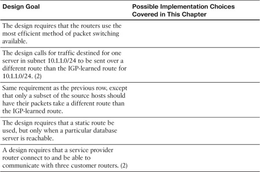
Table 11-5 Design Review
Implementation Plan Peer Review Table
Table 11-6 shows a list of questions that others might ask, or that you might think about, during a peer review of another network engineer’s implementation plan. Complete the table by answering the questions.
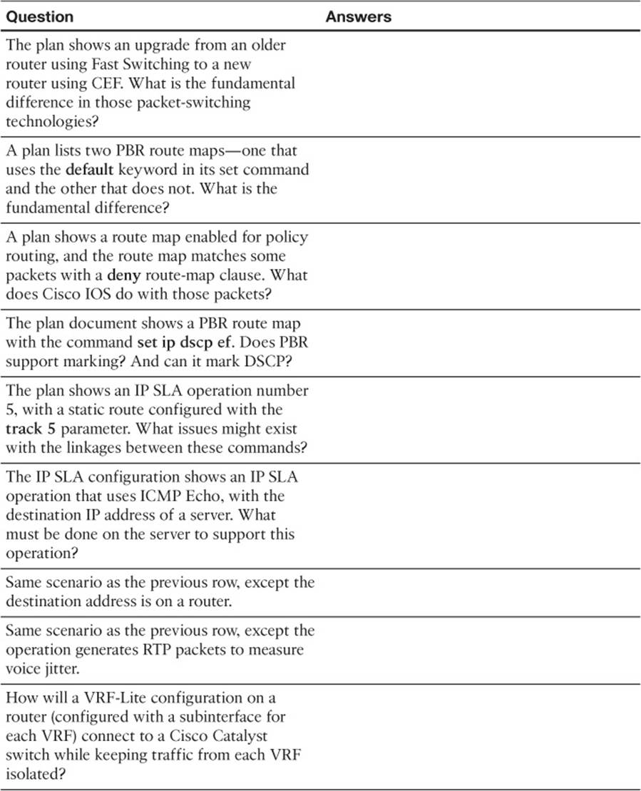
Table 11-6 Notable Questions from This Chapter to Consider During an Implementation Plan Peer Review
Create an Implementation Plan Table
To practice skills useful when creating your own implementation plan, list in Table 11-7 all configuration commands related to the configuration of the following features. You might want to record your answers outside the book and set a goal to complete this table (and others like it) from memory during your final reviews before taking the exam.
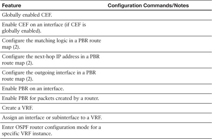
Table 11-7 Implementation Plan Configuration Memory Drill
Choose Commands for a Verification Plan Table
To practice skills useful when creating your own verification plan, list in Table 11-8 all commands that supply the requested information. You might want to record your answers outside the book and set a goal to complete this table (and others like it) from memory during your final reviews before taking the exam.
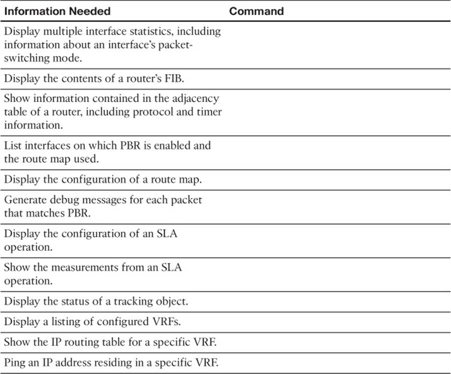
Table 11-8 Verification Plan Memory Drill
Note
Some of the entries in this table might not have been specifically mentioned in this chapter, but are listed in the table for review and reference.
Review All the Key Topics
Review the most important topics from inside the chapter, noted with the Key Topic icon in the outer margin of the page. Table 11-9 lists a reference of these key topics and the page numbers on which each is found.
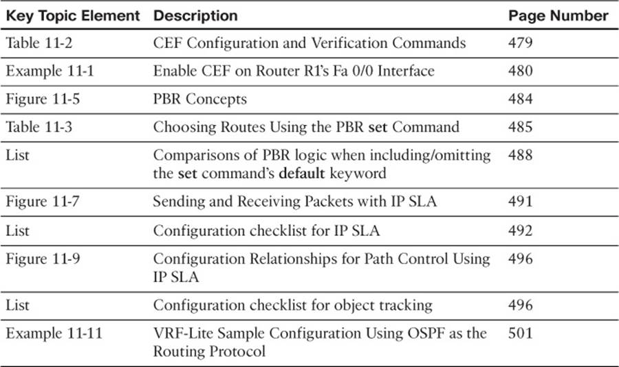
Table 11-9 Key Topics for Chapter 11
Complete the Tables and Lists from Memory
Print a copy of Appendix D, “Memory Tables,” (found on the CD) or at least the section for this chapter, and complete the tables and lists from memory. Appendix E, “Memory Tables Answer Key,” also on the CD, includes completed tables and lists to check your work.
Definitions of Key Terms
Define the following key terms from this chapter, and check your answers in the glossary.
Cisco Express Forwarding
Policy-Based Routing
IP Service-Level Agreement
tracking object
path control
ToS
IP Precedence
SLA Operation
Virtual Routing and Forwarding (VRF)
VRF-Lite