CCNP Routing and Switching ROUTE 300-101 Official Cert Guide (2015)
Part IV. Internet Connectivity
Chapter 14. Advanced BGP Concepts
This chapter covers the following subjects:
![]() Internal BGP Between Internet-Connected Routers: This section examines the need for iBGP peering inside an enterprise, and both the required and the commonly used optional configuration settings.
Internal BGP Between Internet-Connected Routers: This section examines the need for iBGP peering inside an enterprise, and both the required and the commonly used optional configuration settings.
![]() Avoiding Routing Loops When Forwarding Toward the Internet: This section discusses the issues that can occur when Internet-connected routers forward packets to each other through routers that do not use BGP, and how such a design requires some means to supply BGP-learned routes to the internal enterprise routers.
Avoiding Routing Loops When Forwarding Toward the Internet: This section discusses the issues that can occur when Internet-connected routers forward packets to each other through routers that do not use BGP, and how such a design requires some means to supply BGP-learned routes to the internal enterprise routers.
![]() Route Filtering and Clearing BGP Peers: This section gives a brief description of the options for filtering the contents of BGP Updates, along with explaining some operational issues related to the BGP clear command.
Route Filtering and Clearing BGP Peers: This section gives a brief description of the options for filtering the contents of BGP Updates, along with explaining some operational issues related to the BGP clear command.
![]() BGP Path Attributes and Best Path Algorithm: This section describes the BGP Path Attributes (PA) that have an impact on the BGP best path algorithm–the algorithm BGP uses to choose the best BGP route for each destination prefix.
BGP Path Attributes and Best Path Algorithm: This section describes the BGP Path Attributes (PA) that have an impact on the BGP best path algorithm–the algorithm BGP uses to choose the best BGP route for each destination prefix.
![]() Influencing an Enterprise’s Outbound Routes: This section shows how to use the BGP features that influence the BGP best path algorithm.
Influencing an Enterprise’s Outbound Routes: This section shows how to use the BGP features that influence the BGP best path algorithm.
![]() Influencing an Enterprise’s Inbound Routes with MED: This section shows how to use the Multi-Exit Discriminator (MED) BGP feature that influences the BGP best path algorithm for inbound routes.
Influencing an Enterprise’s Inbound Routes with MED: This section shows how to use the Multi-Exit Discriminator (MED) BGP feature that influences the BGP best path algorithm for inbound routes.
Outbound routing is simple with a single Internet-connected router. An enterprise interior gateway protocol (IGP) could flood a default route throughout the enterprise, funneling all Internet traffic toward the one Internet-connected router. That router could then choose the best route to any and all Internet destinations it learned with external BGP (eBGP).
With two (or more) Internet-connected routers in a single enterprise, additional issues arise; in particular, issues related to outbound routing. These issues require the use of Border Gateway Protocol (BGP) between enterprise routers. In some cases, the design might require BGP even on enterprise routers that do not peer with routers at the various Internet service providers (ISP). This chapter examines the scenarios in which using internal BGP (iBGP) makes sense, and shows the related configuration and verification commands.
This chapter begins by focusing on the issues that can occur when an enterprise uses a pair of Internet-connected routers. Specifically, the examples use the sample network shown in Figure 14-1. This design uses the same ISPs and ISP routers as in Chapter 13, “Fundamental BGP Concepts,” with familiar IP address ranges but with a few different links. The design now also shows two of the core routers (actually Layer 3 switches) inside the enterprise—routers that do not directly connect to any ISP. Figure 14-1 shows the design that will be referenced in the first few sections of this chapter.
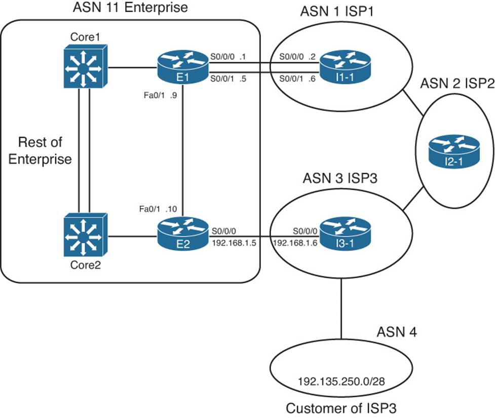
Figure 14-1 Dual Internet Router Design Used in Chapter 14
Note
Figure 14-1 shows the IP addresses as just the last octet of the address; in these cases, the first three octets are 10.1.1.
The first section of this chapter focuses on concepts, configuration, and verification of the iBGP connection between E1 and E2 in the figure. The second major section of this chapter, “Avoiding Routing Loops When Forwarding Toward the Internet,” examines the need for iBGP on routers internal to the enterprise, such as Routers Core1 and Core2 in the figure. The third section of this chapter examines the process of filtering both iBGP and eBGP routing updates.
IGPs choose the best route based on some very straightforward concepts. Routing Information Protocol (RIP) uses the least number of router hops between a router and the destination subnet. Enhanced Interior Gateway Routing Protocol (EIGRP) uses a formula based on a combination of the constraining bandwidth and least delay, and Open Shortest Path First (OSPF) uses lowest cost with that cost based on bandwidth.
BGP uses a much more detailed process to choose the best BGP route. BGP does not consider router hops, bandwidth, or delay when choosing the best route to reach each subnet. Instead, BGP defines several items to compare about the competing routes, in a particular order. Some of these comparisons use BGP features that can be set based on the router configuration, allowing network engineers to then influence which path BGP chooses as the best path.
BGP’s broader set of tools allows much more flexibility when influencing the choice of best route. This BGP best-path process also requires only simple comparisons by the router to choose the best route for a prefix. Although the detail of the BGP best-path selection process requires more work to understand, that complexity gives engineers additional design and implementation options, and gives engineers many options to achieve their goals when working with the large interconnected networks that comprise the Internet.
This chapter completes the BGP coverage in this book by examining the topic of BGP Path Control, including BGP Path Attributes, the BGP Best Path selection process, along with a discussion of how to use four different features to influence the choice of best path by setting BGP Path Attribute (PA) values.
“Do I Know This Already?” Quiz
The “Do I Know This Already?” quiz allows you to assess whether you should read the entire chapter. If you miss no more than two of these 14 self-assessment questions, you might want to move ahead to the “Exam Preparation Tasks” section. Table 14-1 lists the major headings in this chapter and the “Do I Know This Already?” quiz questions covering the material in those headings so that you can assess your knowledge of these specific areas. The answers to the “Do I Know This Already?” quiz appear in Appendix A.
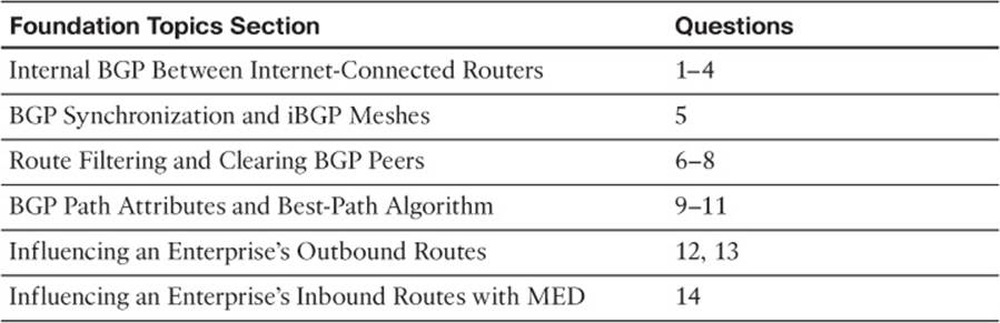
Table 14-1 “Do I Know This Already?” Foundation Topics Section-to-Question Mapping
1. R1 in ASN 1 with loopback1 address 1.1.1.1 needs to be configured with an iBGP connection to R2 with loopback2 IP address 2.2.2.2. The connection should use the loopbacks. Which of the following commands is required on R1?
a. neighbor 1.1.1.1 remote-as 1
b. neighbor 2.2.2.2 remote-as 2
c. neighbor 2.2.2.2 update-source loopback1
d. neighbor 2.2.2.2 ibgp-multihop 2
e. neighbor 2.2.2.2 ibgp-mode
2. The following output occurred as a result of the show ip bgp command on Router R1. The output shows all BGP table entries on R1. How many iBGP-learned routes exist on this router?
*>i181.0.0.0/8 10.100.1.1 0 100 0 1 2 111 112 i
*>i182.0.0.0/8 10.100.1.1 0 100 0 1 2 222 i
*>i183.0.0.0/8 10.100.1.1 0 100 0 1 2 i
*>i184.0.0.0/8 10.100.1.1 0 100 0 1 2 i
*> 192.135.250.0/28 192.168.1.6 0 3 4 i
a. 1
b. 2
c. 3
d. 4
e. 5
3. The following output on Router R1 lists details of a BGP route for 190.1.0.0/16. Which of the following are true based on this output? (Choose two.)
R1# show ip bgp 190.1.0.0/16
BGP routing table entry for 190.1.0.0/16, version 121
Paths: (1 available, best #1, table Default-IP-Routing-Table)
Advertised to update-groups:
1
1 2 3 4
1.1.1.1 from 2.2.2.2 (3.3.3.3)
Origin IGP, metric 0, localpref 100, valid, internal, best
a. R1 has a neighbor 1.1.1.1 command configured.
b. R1 has a neighbor 2.2.2.2 command configured.
c. The show ip bgp command lists a line for 190.1.0.0/16 with both an > and an i on the left.
d. R1 is in ASN 1.
4. A company uses Routers R1 and R2 to connect to ISP1 and ISP2, respectively, with Routers I1 and I2 used at the ISPs. R1 peers with I1 and R2. R2 peers with I2 and R1. Assuming that as many default settings as possible are used on all four routers, which of the following is true about the next-hop IP address for routes R1 learns over its iBGP connection to R2?
a. The next hop is I2’s BGP RID.
b. The next hop is I2’s IP address used on the R2-I2 neighbor relationship.
c. The next hop is R2’s BGP RID.
d. The next hop is R2’s IP address used on the R1-R2 neighbor relationship.
5. A company uses Routers R1 and R2 to connect to ISP1 and ISP2, respectively, with Routers I1 and I2 used at the ISPs. R1 peers with I1 and R2. R2 peers with I2 and R1. R1 and R2 do not share a common subnet, relying on other routers internal to the enterprise for IP connectivity between the two routers. Which of the following could be used to prevent potential routing loops in this design? (Choose two.)
a. Using an iBGP mesh inside the enterprise core
b. Configuring default routes in the enterprise pointing to both R1 and R2
c. Redistributing BGP routes into the enterprise IGP
d. Tunneling the packets for the iBGP connection between R1 and R2
6. R1 is currently advertising prefixes 1.0.0.0/8, 2.0.0.0/8, and 3.0.0.0/8 over its eBGP connection to neighbor 2.2.2.2 (R2). An engineer configures a prefix list (fred) on R1 that permits only 2.0.0.0/8 and then enables the filter with the neighbor R2 prefix-list fred out command. Upon exiting configuration mode, the engineer uses some show commands on R1, but no other commands. Which of the following is true in this case?
a. The show ip bgp neighbor 2.2.2.2 received-routes command lists the three original prefixes.
b. The show ip bgp neighbor 2.2.2.2 advertised-routes command lists the three original prefixes.
c. The show ip bgp neighbor 2.2.2.2 routes command lists the three original prefixes.
d. The show ip bgp neighbor 2.2.2.2 routes command lists only 2.0.0.0/8.
e. The show ip bgp neighbor 2.2.2.2 advertised-routes command lists only 2.0.0.0/8.
7. Which of the following BGP filtering methods enabled with the neighbor command will filter BGP prefixes based on the prefix and prefix length? (Choose three.)
a. A neighbor distribute-list out command, referencing a standard ACL
b. A neighbor prefix-list out command
c. A neighbor filter-list out command
d. A neighbor distribute-list out command, referencing an extended ACL
e. A neighbor route-map out command
8. Which of the following commands cause a router to bring down BGP neighbor relationships? (Choose two.)
a. clear ip bgp *
b. clear ip bgp 1.1.1.1
c. clear ip bgp * soft
d. clear ip bgp 1.1.1.1 out
9. An engineer is preparing an implementation plan in which the configuration needs to influence BGP’s choice of best path. Which of the following is least likely to be used by the configuration in this implementation plan?
a. Weight
b. Origin code
c. AS_Path
d. Local_Pref
10. Router R1 learns two routes with BGP for prefix 200.1.0.0/16. Comparing the two routes, route 1 has a longer AS_Path Length, bigger MED, bigger Weight, and smaller Local Preference. Which of the following is true about Router R1’s choice of best path for this prefix?
a. Route 1 is the best route.
b. Route 2 is the best route.
c. The routes tie as best, but one will be picked to be placed in the routing table based on tiebreakers.
d. Neither route is considered best.
11. Router R1 learns two routes with BGP for prefix 200.1.0.0/16. Comparing the two routes, route 1 has a shorter AS_Path Length, smaller MED, the same Weight, and smaller Local Preference. Which of the following is true about Router R1’s choice of best path for this prefix?
a. Route 1 is the best route.
b. Route 2 is the best route.
c. The routes tie as best, but one will be picked to be placed in the routing table based on tiebreakers.
d. Neither route is considered best.
12. An engineer has been told to create an implementation plan to influence the choice of best BGP route on a single router using the Weight feature. The sole enterprise Internet-connected router, Ent1, has neighbor relationships with Routers ISP1 and ISP2, which reside inside two different ISPs. The goal is to prefer all routes learned from ISP1 over ISP2 using Weight. Which of the following answers list a configuration step that would not be useful for achieving these goals? (Choose two.)
a. Configuring the neighbor weight command on Ent1
b. Having the ISPs configure the neighbor route-map out command on ISP1 and ISP2, with the route map setting the Weight
c. Configuring the set weight command inside a route map on Router Ent1
d. Configuring a prefix list to match all Class C networks
13. An enterprise router, Ent1, displays the following excerpt from the show ip bgp command. Ent1 has an eBGP connection to an ISP router with address 3.3.3.3 and an iBGP connection to a router with address 4.4.4.4. Which of the following is most likely to be true?
Network Next Hop Metric LocPrf Weight Path
*> 3.3.3.3 0 0 1 1 1 1 2 18 i
a. The enterprise likely uses ASN 1.
b. The neighboring ISP likely uses ASN 1.
c. The route has been advertised through ASN 1 multiple times.
d. Router Ent1 will add another ASN to the AS_Path before advertising this route to its iBGP peer (4.4.4.4).
14. The following line of output was gathered on enterprise Router Ent1 using the command show ip route. Which of the following answers is most likely to be true, based on this output?
B 128.107.0.0 [20/10] via 11.11.11.11, 00:02:18
a. This router has set the Weight of this route to 10.
b. This router’s BGP table lists this route as an iBGP route.
c. This router’s MED has been set to 10.
d. This router’s BGP table lists an AS_Path length of 10 for this route.
Foundation Topics
Internal BGP Between Internet-Connected Routers
When an enterprise uses more than one router to connect to the Internet, and those routers use BGP to exchange routing information with their ISPs, those same routers need to exchange BGP routes with each other as well. The BGP neighbor relationships occur inside that enterprise—inside a single AS—making these routers iBGP peers.
This first major section of this chapter begins with a look at why two Internet-connected routers need to have an iBGP neighbor relationship. Then, the text looks at various iBGP configuration and verification commands. Finally, the discussion turns to a common issue that occurs with next-hop reachability between iBGP peers, with an examination of the options to overcome the problem.
Establishing the Need for iBGP with Two Internet-Connected Routers
Two Internet-connected routers in an enterprise need to communicate BGP routes to each other, because these routers might want to forward IP packets to the other Internet-connected router, which in turn would forward the packet to the Internet. With an iBGP peer connection, each Internet-connected router can learn routes from the other router and decide whether that other router has a better route to reach some destinations in the Internet. Without that iBGP connection, the routers have no way to know whether the other router has a better BGP path.
For example, consider Figure 14-2, which shows two such cases.
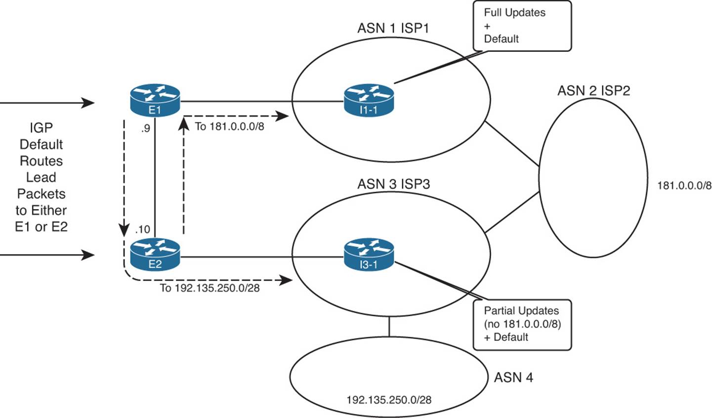
Figure 14-2 Choosing the Best Routes from ASN 11 to 181.0.0.0/8 and 192.135.250.0/28
The figure shows a topology that uses the following design options, as agreed upon with ISP1 and ISP3:
![]() ISP1 sends full routing updates and a default route.
ISP1 sends full routing updates and a default route.
![]() ISP3 sends partial updates and a default route.
ISP3 sends partial updates and a default route.
First, consider the eBGP routing updates, particularly for the two prefixes highlighted in the figure. Both ISP1 and ISP3 know routes for 181.0.0.0/8, but ISP3’s agreement with the enterprise is that ISP3 sends partial updates. This usually means that ISP3 sends updates for prefixes in its own autonomous system number (ASN) plus prefixes for customers attached to its ASN, such as 192.135.250.0/28 in this case. ISP1, however, sends full updates. So, E1 learns an eBGP route for both 181.0.0.0/8 and 192.135.250.0/28, but Router E2 only learns an eBGP route for 192.135.250.0/28.
Next, take a closer look at the routes for 181.0.0.0/8, both on E1 and E2. Only E1 learns an eBGP route for 181.0.0.0/8; E2 does not, because of ISP3’s partial updates. If E1 and E2 did not use iBGP between each other, E2 would never know that E1 had a good route for 181.0.0.0/8. Without an iBGP connection, packets destined to hosts in 181.0.0.0/8, if they arrived at E2, would be sent to ISP3 because of E2’s default route learned from ISP3. However, if E1 and E2 form an iBGP neighbor relationship, E2 would know a route for 181.0.0.0/8 through E1 and would choose this route as its best route and would forward such packets to E1. Then E1 would forward the packets to ISP1, as shown in the figure.
Finally, take a closer look at the routes for 192.135.250.0/28 on both E1 and E2. If none of the ISPs changed the default PA settings for these routes, both E1 and E2 would choose the route through E2 as the better route, because of the shorter AS_Path length (two ASNs away through ISP3 versus four ASNs away through ISP1). Without iBGP between E1 and E2, E1 would not learn of this better route through E2. So, any packets destined to 192.135.250.0/28 that reach E1 would be forwarded to ISP1. With iBGP, E1 would know of E2’s better route and forward the packets toward E2, as shown in the figure.
For both prefixes, iBGP allowed both routers in the same ASN to reach the same conclusion about the better router through which to send packets for each Internet destination.
Configuring iBGP
The most basic iBGP configuration differs only slightly compared to eBGP configuration. The configuration does not explicitly identify an eBGP versus an iBGP peer. Instead, for iBGP, the neighbor’s ASN listed on the neighbor neighbor-ip remote-as neighbor-asn command lists the same ASN as the local router’s router bgp command. eBGP neighbor remote-as commands list a different ASN.
When two iBGP peers share a common physical link, such as E1 and E2 in Figure 14-2, the iBGP configuration simply requires a single neighbor remote-as command on each router. Example 14-1 shows the BGP configuration on both Router E1 and E2 with this single neighbor command highlighted. The rest of the configuration lists the commands used to configure other BGP settings (as described after the example). Note that Figure 14-1 in the introduction to this chapter shows more detail about the eBGP peers.
Example 14-1 BGP Configuration on E1: Neighborships Configured
! Configuration on router E1
router bgp 11
no synchronization
bgp log-neighbor-changes
aggregate-address 128.107.0.0 255.255.224.0 summary-only
redistribute ospf 1 route-map only-128-107
neighbor 1.1.1.1 remote-as 1
neighbor 1.1.1.1 password fred
neighbor 1.1.1.1 ebgp-multihop 2
neighbor 1.1.1.1 update-source Loopback1
neighbor 10.1.1.10 remote-as 11
no auto-summary
!
! Next, static routes so that the eBGP neighbor packets can reach
! I1-1's loopback interface address 1.1.1.1
ip route 1.1.1.1 255.255.255.255 Serial0/0/0
ip route 1.1.1.1 255.255.255.255 Serial0/0/1
!
ip prefix-list 128-107 seq 5 permit 128.107.0.0/19 le 32
!
route-map only-128-107 permit 10
match ip address prefix-list 128-107
! Now, on router E2
router bgp 11
no synchronization
bgp log-neighbor-changes
network 128.107.32.0
aggregate-address 128.107.0.0 255.255.224.0 summary-only
redistribute ospf 1 route-map only-128-107
neighbor 10.1.1.9 remote-as 11
neighbor 192.168.1.6 remote-as 3
neighbor 192.168.1.6 password barney
no auto-summary
!
ip prefix-list 128-107 seq 5 permit 128.107.0.0/19 le 32
!
route-map only-128-107 permit 10
match ip address prefix-list 128-107
Only the four highlighted configuration commands are required for the E1-E2 iBGP peering. Both refer to the other router’s IP address on the FastEthernet link between the two routers, and both refer to ASN 11. The two routers then realize that the neighbor is an iBGP neighbor, because the neighbor’s ASN (11) matches the local router’s ASN, as seen on the router bgp 11 command.
The example also lists the rest of the BGP configuration. Focusing on Router E1, the configuration basically matches the configuration of Router E1 from the end of Chapter 13, except that E1 has only one eBGP peer (I1-1) in this case, instead of two eBGP peers. The configuration includes the eBGP peer connection to I1-1, using loopback interfaces (1.1.1.1 on I1-1 and 11.11.11.11 on E1). The eBGP peers need to use eBGP multihop because of the use of the loopbacks, and they use message digest algorithm 5 (MD5) authentication as well. Finally, the configuration shows the redistribution of the enterprise’s public address range of 128.107.0.0/19 by redistributing from OSPF and summarizing with the aggregate-address BGP subcommand.
E2’s configuration lists the same basic parameters, but with a few differences. E2 does not use a loopback for its peer connection to I3-1, because only a single link exists between the two routers. As a result, E2 also does not need to use eBGP multihop.
Refocusing on the iBGP configuration, Example 14-1 uses the interface IP addresses of the links between Routers E1 and E2. However, often the Internet-connected routers in an enterprise do not share a common subnet. For example, the two routers might be in separate buildings in a campus for the sake of redundancy. The two routers might actually be in different cities, or even different continents. In such cases, it makes sense to configure the iBGP peers using a loopback IP address for the TCP connection so that a single link failure does not cause the iBGP peer connection to fail. For example, in Figure 14-1, if the FastEthernet link between E1 and E2 fails, the iBGP connection defined in Example 14-1, which uses the interface IP addresses of that link, would fail even though a redundant IP path exists between E1 and E2.
The configuration to use loopback interfaces as the update source mirrors that same configuration for eBGP peers, except that iBGP peers do not need to configure the neighbor neighbor-ip ebgp-multihop command. One difference between iBGP and eBGP is that Cisco IOS uses the low TTL of 1 for eBGP connections by default but does not for iBGP connections. So, for iBGP connections, only the following steps are required to make two iBGP peers use a loopback interface:

Step 1. Configure an IP address on a loopback interface on each router.
Step 2. Configure each router to use the loopback IP address as the source IP address, for the neighborship with the other router, using the neighbor neighbor-ip update-source interface-id command.
Step 3. Configure the BGP neighbor command on each router to refer to the other router’s loopback IP address as the neighbor IP address in the neighbor neighbor-ip remote-as command.
Step 4. Make sure that each router has IP routes so that they can forward packets to the loopback interface IP address of the other router.
Example 14-2 shows an updated iBGP configuration for Routers E1 and E2 to migrate to use a loopback interface. In this case, E1 uses loopback IP address 10.100.1.1/32 and E2 uses 10.100.1.2/32. OSPF on each router has already been configured with a network 10.0.0.0 0.255.255.255 area 0 command (not shown), which causes OSPF to advertise routes to reach the respective loopback interface IP addresses.
Example 14-2 iBGP Configuration to Use Loopbacks as the Update Source
! Configuration on router E1
interface loopback 0
ip address 10.100.1.1 255.255.255.255
router bgp 11
neighbor 10.100.1.2 remote-as 11
neighbor 10.100.1.2 update-source loopback0
! Configuration on router E2
interface loopback 1
ip address 10.100.1.2 255.255.255.255
router bgp 11
neighbor 10.100.1.1 remote-as 11
neighbor 10.100.1.1 update-source loopback1
The highlighted portions of the output link the key values together for the E1’s definition of its loopback as the update source and E2’s reference of that same IP address on its neighbor command. The neighbor 10.100.1.2 update-source loopback0 command on E1 tells E1 to look to interface loopback0 for its update source IP address. Loopback0’s IP address on E1 has IP address 10.100.1.1. Then, E2’s neighbor commands for Router E1 all refer to that same 10.100.1.1 IP address, meeting the requirement that the update source on one router matches the IP address listed on the other router’s neighbor command.
Verifying iBGP
iBGP neighbors use the same messages and neighbor states as eBGP peers. As a result, the same commands in Chapter 13 for BGP neighbor verification can be used for iBGP peers. Example 14-3 shows a couple of examples, using Router E1’s iBGP neighbor relationship with E2 (10.100.1.2) based on the configuration in Example 14-2.
Example 14-3 Verifying iBGP Neighbors
E1# show ip bgp summary
BGP router identifier 11.11.11.11, local AS number 11
BGP table version is 190, main routing table version 190
11 network entries using 1452 bytes of memory
14 path entries using 728 bytes of memory
11/7 BGP path/bestpath attribute entries using 1628 bytes of memory
7 BGP AS-PATH entries using 168 bytes of memory
0 BGP route-map cache entries using 0 bytes of memory
0 BGP filter-list cache entries using 0 bytes of memory
Bitfield cache entries: current 3 (at peak 4) using 96 bytes of memory
BGP using 4072 total bytes of memory
BGP activity 31/20 prefixes, 100/86 paths, scan interval 60 secs
Neighbor V AS MsgRcvd MsgSent TblVer InQ OutQ Up/Down State/PfxRcd
1.1.1.1 4 1 339 344 190 0 0 00:28:41 7
10.100.1.2 4 11 92 132 190 0 0 01:02:04 3
E1# show ip bgp neighbors 10.100.1.2
BGP neighbor is 10.100.1.2, remote AS 11, internal link
BGP version 4, remote router ID 10.100.1.2
BGP state = Established, up for 01:02:10
Last read 00:00:37, last write 00:00:59, hold time is 180, keepalive interval is
60 seconds
Neighbor capabilities:
Route refresh: advertised and received(new)
Address family IPv4 Unicast: advertised and received
! lines omitted for brevity
The show ip bgp summary command lists E1’s two neighbors. As with eBGP peers, if the last column (the State/PfxRcd column) lists a number, the neighbor has reached the established state, and BGP Update messages can be sent. The output can distinguish between an iBGP or eBGP neighbor but only by comparing the local router’s ASN (in the first line of output) to the ASN listed in each line at the bottom of the output.
The show ip bgp neighbors 10.100.1.2 command lists many details specifically for the neighbor. Specifically, it states that the neighbor is an iBGP neighbor with the phrase “internal link,” as highlighted in the output.
Examining iBGP BGP Table Entries
To better understand the BGP table with two (or more) Internet-connected routers inside the same company, start with one prefix and compare the BGP table entries on the two routers for that one prefix. By examining several such examples, you can appreciate more about the benefits and effects of these iBGP neighborships.
This section examines the BGP tables on Routers E1 and E2, focusing on the prefixes highlighted in Figure 14-2—namely, prefixes 181.0.0.0/8 and 192.135.250.0/28. To make reading the output of the show commands a little more obvious, Figure 14-3 collects some key pieces of information into a single figure. This figure shows the two BGP neighbor relationships on each router, showing the update source and neighbor IP address of each BGP neighbor relationship. It also lists the BGP router ID (RID) of the routers.
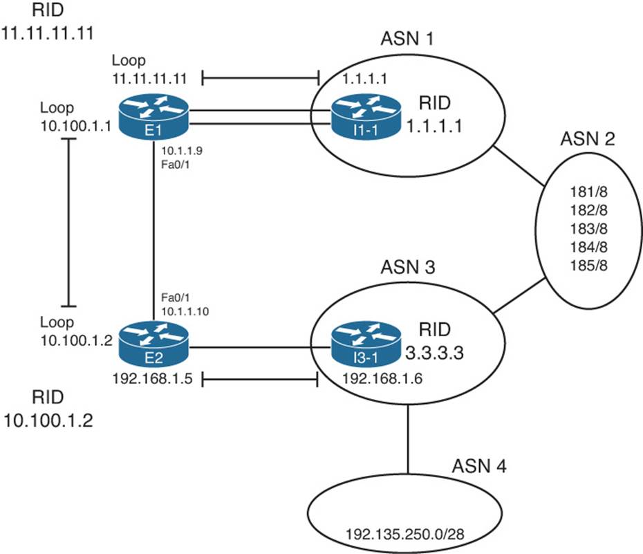
Figure 14-3 Reference Information for BGP Table Verification
Examples 14-4 and 14-5 compare the output on Routers E2 and E1 for prefix 181.0.0.0/8. Example 14-4 lists output on Router E2, listing the BGP table entries for prefix 181.0.0.0/8. Remember, the design calls for ISP3 to only send partial updates, so E2 has not received an eBGP route for 181.0.0.0/8 from I3-1. However, E1 has indeed learned of that prefix from I1-1 (ISP1), and E1 has already advertised prefix 181.0.0.0/8 to E2.
Note
Several BGP routes seen in the examples in this chapter originate in ASNs not shown in the figure. The figure shows enough of the topology to understand the first few ASNs in the AS_Path for these routes.
Example 14-4 Notations of iBGP-Learned Routes in the show ip bgp Command
E2# show ip bgp 181.0.0.0/8 longer-prefixes
BGP table version is 125, local router ID is 10.100.1.2
Status codes: s suppressed, d damped, h history, * valid, > best, i - internal,
r RIB-failure, S Stale
Origin codes: i - IGP, e - EGP, ? - incomplete
Network Next Hop Metric LocPrf Weight Path
*>i181.0.0.0/8 1.1.1.1 0 100 0 1 2 111 112 i
E2# show ip bgp 181.0.0.0/8
BGP routing table entry for 181.0.0.0/8, version 121
Paths: (1 available, best #1, table Default-IP-Routing-Table)
Advertised to update-groups:
1
1 2 111 111
1.1.1.1 from 10.100.1.1 (11.11.11.11)
Origin IGP, metric 0, localpref 100, valid, internal, best
The first command, show ip bgp 181.0.0.0/8 longer-prefixes, lists output with the same general format as the show ip bgp command, but it limits the output to the prefixes in the listed range. Only one such route exists in this case. The legend information at the top of the output, plus the headings and meanings of the different fields, is the same as with the show ip bgp command.
Next, the first command’s output denotes this route as an iBGP-learned route with code “i” in the third character. The second command in the example, show ip bgp 181.0.0.0/8, displays a more detailed view of the BGP table entry and denotes this route as iBGP-learned with the word “internal.” Similarly, the briefer show ip bgp 181.0.0.0/8 command output lists this one route as E2’s best route by displaying a “>” in the second column, whereas the more verbose output in the second command simply lists this route as “best.”
Next, consider these same commands on Router E1, as shown in Example 14-5. Comparing the highlighted fields as matched in each of the examples:
![]() Both list the same AS_Path (1, 2, 111, 112), because iBGP peers do not add ASNs to the AS_Path when advertising to each other. So, both E1 and E2 have the same perspective on the AS_Path and AS_Path length.
Both list the same AS_Path (1, 2, 111, 112), because iBGP peers do not add ASNs to the AS_Path when advertising to each other. So, both E1 and E2 have the same perspective on the AS_Path and AS_Path length.
![]() Both list the one route for 181.0.0.0/8 as the best path, in part because each has learned only one such path.
Both list the one route for 181.0.0.0/8 as the best path, in part because each has learned only one such path.
![]() Both list a Next_Hop (a BGP PA) as 1.1.1.1, which is I1-1’s loopback interface used in the E1–to–I1-1 BGP neighbor relationship (also called the BGP neighbor ID).
Both list a Next_Hop (a BGP PA) as 1.1.1.1, which is I1-1’s loopback interface used in the E1–to–I1-1 BGP neighbor relationship (also called the BGP neighbor ID).
![]() E2 lists the route as an internal (iBGP-learned) route, whereas E1 lists it as an external route.
E2 lists the route as an internal (iBGP-learned) route, whereas E1 lists it as an external route.
Example 14-5 Router E1’s show Commands for BGP Routes for 181.0.0.0/8
E1# show ip bgp 181.0.0.0/8 longer-prefixes
BGP table version is 190, local router ID is 11.11.11.11
Status codes: s suppressed, d damped, h history, * valid, > best, i - internal,
r RIB-failure, S Stale
Origin codes: i - IGP, e - EGP, ? - incomplete
Network Next Hop Metric LocPrf Weight Path
*> 181.0.0.0/8 1.1.1.1 0 1 2 111 112 i
E1# show ip bgp 181.0.0.0/8
BGP routing table entry for 181.0.0.0/8, version 181
Paths: (1 available, best #1, table Default-IP-Routing-Table)
Advertised to update-groups:
2
1 2 111 111, (received & used)
1.1.1.1 from 1.1.1.1 (1.1.1.1)
Origin IGP, localpref 100, valid, external, best
The output from these examples confirms that E1 learned the eBGP route for 181.0.0.0/8 and advertised it to E2, and E2 chose to use that iBGP-learned route as its best route to reach 181.0.0.0/8.
Next, consider the route for 192.135.250.0/28, a route learned in the full BGP updates from ISP1’s Router I1-1 and in the partial BGP updates from ISP3’s Router I3-1. After exchanging this route using their iBGP peering, both E1 and E2 should see two possible routes: an eBGP route learned from their one connected ISP and the iBGP route learned from each other. Again assuming that the ISPs have not made any attempt to set PA values to influence the best-path choice, and knowing that neither E1 nor E2 have configured BGP to influence the best-path choice, the route through E2 should be best because of the shorter AS_Path.
Example 14-6 shows the output of the show ip bgp command on both E1 and E2, again for comparison. Note that the command used in the examples, show ip bgp 192.135.250.0/28 longer-prefixes, is used, because it lists only the routes for that prefix, rather than the full BGP table displayed by show ip bgp. However, the format of the output is almost identical.
Example 14-6 Comparing BGP Routes for 192.135.250.0/28 on E1 and E2
! First, on E1:
E1# show ip bgp 192.135.250.0/28 longer-prefixes
BGP table version is 26, local router ID is 128.107.9.1
Status codes: s suppressed, d damped, h history, * valid, > best, i - internal,
r RIB-failure, S Stale
Origin codes: i - IGP, e - EGP, ? - incomplete
Network Next Hop Metric LocPrf Weight Path
* 192.135.250.0/28 1.1.1.1 0 1 2 3 4 i
*>i 192.168.1.6 0 100 0 3 4 i
! Next, on E2:
E2# show ip bgp 192.135.250.0/28 longer-prefixes
BGP table version is 25, local router ID is 10.100.1.2
Status codes: s suppressed, d damped, h history, * valid, > best, i - internal,
r RIB-failure, S Stale
Origin codes: i - IGP, e - EGP, ? - incomplete
Network Next Hop Metric LocPrf Weight Path
*> 192.135.250.0/28 192.168.1.6 0 3 4 i
First, E1 lists two routes for this prefix, one external and one internal. The output identifies external routes by the absence of an “i” in the third character, whereas the output lists an “i” in the third character for internal routes. In this case, E1’s internal route, with Next_Hop 192.168.1.6, is E1’s best route, as was shown back in Figure 14-2. E1 chose this iBGP route because of the shorter AS_Path length; the AS_Path is highlighted at the end of each line.
E2’s output in the second half of Example 14-6 lists only a single route—its eBGP route for 192.135.250.0/28. That only one route appears, rather than two, is a good example of the effect of two rules about how BGP operates:
![]() Only advertise the best route in any BGP Update.
Only advertise the best route in any BGP Update.
![]() Do not advertise iBGP-learned routes to iBGP peers.
Do not advertise iBGP-learned routes to iBGP peers.
E2’s output lists a single route for 192.135.250.0/28—its external route learned from ISP3—because E1 chooses not to advertise a route for 192.135.250.0/28 over the iBGP connection. If you look back at E1’s output, E1’s best route for this prefix is its internal route. So, if E1 were to advertise any route for this prefix to E2, E1 would advertise this internal route, because it is E1’s best BGP route for that prefix. However, the second rule—do not advertise iBGP-learned routes to iBGP peers—prevents E1 from advertising this route back to E2. (Logically speaking, it makes no sense for E1 to tell E2 about a route when E2 is the router that originally advertised the route to E1 in the first place—a concept much like Split Horizon, although technically the term does not apply to BGP.) As a result, E2 lists a single route for 192.135.250.0/28.
Note that if the route for 192.135.250.0/28 through ISP3 failed, E1 would start using the route through ISP1 as its best route. E1 would then advertise that best route to E2 that could then forward traffic through E1 for destinations in 192.135.250.0/28.
Understanding Next-Hop Reachability Issues with iBGP
With IGPs, the IP routes added to the IP routing table list a next-hop IP address. With few exceptions, the next-hop IP address exists in a connected subnet. For example, the E1-E2 iBGP connection uses loopback interfaces 10.100.1.1 (E1) and 10.100.1.2 (E2). E1’s OSPF-learned route to reach 10.100.1.2 lists outgoing interface Fa0/1, next-hop 10.1.1.10—an address in the LAN subnet that connects E1 and E2. (See Figure 14-3 a few pages back for reference.)
Examples 14-5 and 14-6 also happened to show two examples of iBGP-learned routes and their next-hop addresses. The next-hop addresses were not in connected subnets; the next-hop addresses were not even IP addresses on a neighboring router. The two examples were as follows; again, it might be helpful to refer to the notations in Figure 14-3:
![]() Example 14-5: E2’s route for 181.0.0.0/8 lists next-hop address 1.1.1.1, a loopback interface IP address on I1-1.
Example 14-5: E2’s route for 181.0.0.0/8 lists next-hop address 1.1.1.1, a loopback interface IP address on I1-1.
![]() Example 14-6: E1’s route for 192.135.250.0/28 lists next-hop address 192.168.1.6, which is I3-1’s interface IP address on the link between E2 and I3-1.
Example 14-6: E1’s route for 192.135.250.0/28 lists next-hop address 192.168.1.6, which is I3-1’s interface IP address on the link between E2 and I3-1.
In fact, in the case of Example 14-5, the output of the show ip bgp 181.0.0.0/8 command on E2 listed the phrase “1.1.1.1 from 10.100.1.1 (11.11.11.11).” This phrase lists the next hop (1.1.1.1) of the route, the neighbor from which the route was learned (10.100.1.1 or E1), and the neighbor’s BGP RID (11.11.11.11, as listed in Figure 14-3).
BGP advertises these particular IP addresses as the next-hop IP addresses because of a default behavior for BGP. By default, when a router advertises a route using eBGP, the advertising router lists its own update-source IP address as the next-hop address of the route. In other words, the next-hop IP address is the IP address of the eBGP neighbor, as listed on the neighbor remote-as command. However, when advertising a route to an iBGP peer, the advertising router (by default) does not change the next-hop address. For example, when I1-1 advertises 181.0.0.0/8 to E1, because it is an eBGP connection, I1-1 sets its own IP address (1.1.1.1)—specifically the IP address I1-1 uses on its eBGP peer connection to E1—as the next hop. When E1 advertises that same route to iBGP peer E2, E1 does not change the next-hop address of 1.1.1.1. So, Router E2’s iBGP-learned route lists 1.1.1.1 as the next-hop address.
The IP routing process can use routes whose next-hop addresses are not in connected subnets as long as each router has an IP route that matches the next-hop IP address. Therefore, engineers must understand these rules about how BGP sets the next-hop address and ensure that each router can reach the next-hop address listed in the BGP routes. Two main options exist to ensure reachability to these next-hop addresses:
![]() Create IP routes so that each router can reach these next-hop addresses that exist in other ASNs.
Create IP routes so that each router can reach these next-hop addresses that exist in other ASNs.
![]() Change the default iBGP behavior with the neighbor neighbor-ip next-hop-self command.
Change the default iBGP behavior with the neighbor neighbor-ip next-hop-self command.
The text now examines each of these two options in more detail.
Ensuring That Routes Exist to the Next-Hop Address
Routers can still forward packets using routes whose next-hop addresses are not in connected subnets. To do so, when forwarding packets, the router performs a recursive route table lookup. For example, for packets arriving at E2 with a destination of 181.0.0.1, the following would occur:
Step 1. E2 would match the routing table for destination address 181.0.0.1, matching the route for 181.0.0.0/8, with next hop 1.1.1.1.
Step 2. E2 would next look for its route matching destination 1.1.1.1—the next hop of the first route—and forward the packet based on that route.
So, regardless of the next-hop IP address listed in the routing table, as long as a working route exists to reach that next-hop IP address, the packet can be forwarded. Figure 14-4 shows the necessary routes in diagram form using two examples. E1 has a route to 192.135.250.0/28 with next hop 192.168.1.6; two arrowed lines show the required routes on Routers E1 and E2 for forwarding packets to this next-hop address. Similarly, the dashed lines show the necessary routes on E2 and E1 for next-hop address 1.1.1.1, the next-hop IP address for their routes to reach 181.0.0.0/8.
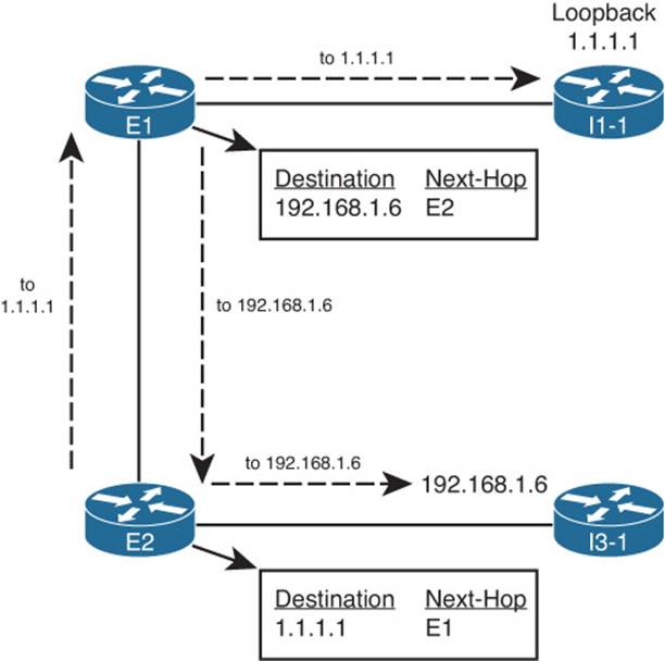
Figure 14-4 Ensuring That Routes Exist for Next-Hop Addresses in Other ASNs
Two easily implemented solutions exist to add routes for these nonconnected next-hop IP addresses: Either add static routes or use an IGP between the enterprise and the ISPs for the sole purpose of advertising these next-hop addresses.
Using neighbor neighbor-ip next-hop-self to Change the Next-Hop Address
The second option for dealing with these nonconnected next-hop IP addresses changes the iBGP configuration so that a router changes the next-hop IP address on iBGP-advertised routes. This option simply requires the neighbor neighbor-ip next-hop-self command to be configured for the iBGP neighbor relationship. A router with this command configured advertises iBGP routes with its own update source IP address as the next-hop IP address. And because the iBGP neighborship already relies on a working route for these update source IP addresses, if the neighborship is up, IP routes already exist for these next-hop addresses.
For example, on the iBGP connection from E1 to E2, E1 would add the neighbor 10.100.1.2 next-hop-self command, and E2 would add the neighbor 10.100.1.1 next-hop-self command. When configured, E1 advertises iBGP routes with its update source IP address (10.100.1.1) as the next-hop address. E2 likewise advertises routes with a next-hop address of 10.100.1.2. Example 14-7 shows E2’s BGP table, with a few such examples highlighted, after the addition of these two configuration commands on the respective routers.
Example 14-7 Seeing the Effects of next-hop-self from Router E2
E2# show ip bgp
BGP table version is 76, local router ID is 10.100.1.2
Status codes: s suppressed, d damped, h history, * valid, > best, i - internal,
r RIB-failure, S Stale
Origin codes: i - IGP, e - EGP, ? - incomplete
Network Next Hop Metric LocPrf Weight Path
*> 0.0.0.0 192.168.1.6 0 0 3 i
* i 10.100.1.1 0 100 0 1 i
* i128.107.0.0/19 10.100.1.1 0 100 0 i
*> 0.0.0.0 32768 i
s> 128.107.1.0/24 10.1.1.77 2 32768 ?
s> 128.107.2.0/24 10.1.1.77 2 32768 ?
s> 128.107.3.0/24 10.1.1.77 2 32768 ?
*>i181.0.0.0/8 10.100.1.1 0 100 0 1 2 111 112 i
*>i182.0.0.0/8 10.100.1.1 0 100 0 1 2 222 i
*>i183.0.0.0/8 10.100.1.1 0 100 0 1 2 i
*>i184.0.0.0/8 10.100.1.1 0 100 0 1 2 i
*>i185.0.0.0/8 10.100.1.1 0 100 0 1 2 i
*> 192.135.250.0/28 192.168.1.6 0 3 4 i
This completes the discussion of iBGP configuration and operation as related to the routers actually connected to the Internet. The next section continues the discussion of iBGP but with a focus on some particular issues with routing that might require iBGP on routers other than the Internet-connected routers.
Avoiding Routing Loops When Forwarding Toward the Internet
A typical enterprise network design uses default routes inside an enterprise, as advertised by an IGP, to draw all Internet traffic toward one or more Internet-connected routers. The Internet-connected routers then forward the traffic into the Internet.
However, as discussed in Chapter 13, in the section “Choosing One Path over Another Using BGP,” routing loops can occur when the Internet-connected routers do not have a direct connection to each other. For example, if the Internet-connected routers sit on opposite sides of the country, the two routers might be separated by several routers internal to the enterprise, because they do not have a direct link.
To show a simple example, the same enterprise network design shown in all previous figures in this chapter can be changed slightly by just disabling the FastEthernet link between the two routers, as shown in Figure 14-5.
Figure 14-5 shows an example of the looping problem.
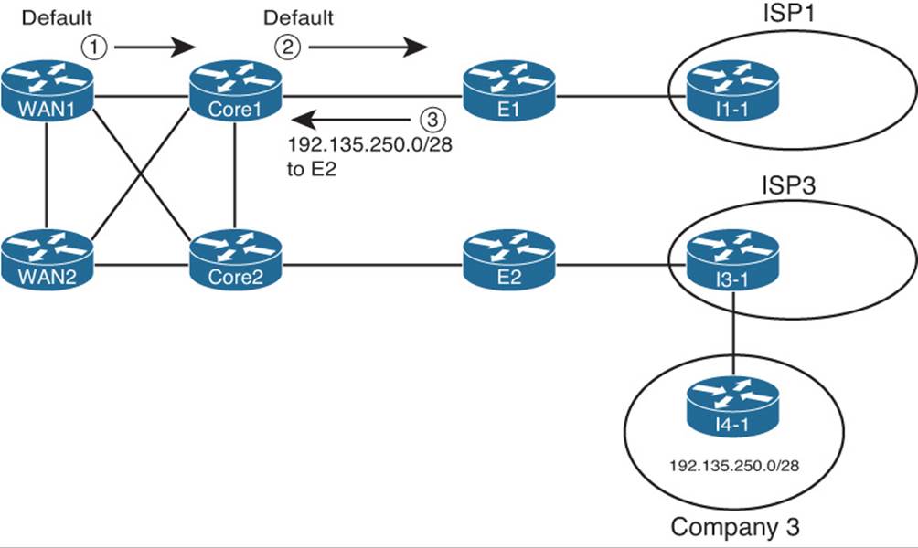
Figure 14-5 Routing Loop for Packets Destined to 192.135.250.1
The figure uses the same general criteria as the other examples in this chapter, such that E1’s best route for 192.135.250.0/28 points to Router E2 as the next hop. E1’s best route for the next-hop IP address for its route to 192.135.250.0/28—regardless of whether using the next-hop-selfoption or not—sends the packet back toward the enterprise core. However, some of (or possibly all) the enterprise routers internal to the enterprise, such as WAN1 and Core1, use a default that sends all packets toward Router E1. Per the steps in the figure, the following happens for a packet destined to 192.135.250.1:
Step 1. WAN1 sends the packet using its default route to Core1.
Step 2. Core1 sends the packet using its default route to E1.
Step 3. E1 matches its BGP route for 192.135.250.0/28, with next-hop E2 (10.100.1.2). The recursive lookup on E1 matches a route for 10.100.1.2 with a next hop of Core1, so E1 sends the packet back to Core1.
At this point, Steps 2 and 3 repeat until the packet’s TTL mechanism causes one of the routers to discard the packet.
The lack of knowledge about the best route for subnet 192.135.250.0/28, particularly on the routers internal to the enterprise, causes this routing loop. To avoid this problem, internal routers, such as Core1 and Core2, need to know the best BGP routes. Two solutions exist to help these internal routers learn the routes:
![]() Run BGP on at least some of the routers internal to the enterprise (such as Core1 and Core2 in Figure 14-5).
Run BGP on at least some of the routers internal to the enterprise (such as Core1 and Core2 in Figure 14-5).
![]() Redistribute BGP routes into the IGP (not recommended).
Redistribute BGP routes into the IGP (not recommended).
Both solutions solve the problem by giving some of the internal routers the same best-path information already known to the Internet-connected routers. For example, if Core1 knew a route for 192.135.250.0/28, and that route caused the packets to go to Core2 next and then on to Router E2, the loop could be avoided. This section examines both solutions briefly.
Note
BGP Confederations and BGP Route Reflector features, which are outside the scope of this book, can be used instead of a full mesh of iBGP peers.
Using an iBGP Mesh
To let the internal routers in the enterprise learn the best BGP routes, one obvious solution is to just run BGP on these routers as well. The not-so-obvious part relates to the implementation choice of what routers need to be iBGP peers with each other. Based on the topology shown in Figure 14-5, at first glance, the temptation might be to run BGP on E1, E2, Core1, and Core2, but use iBGP peers as shown in Figure 14-6.
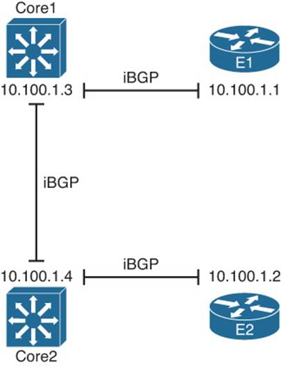
Figure 14-6 Partial Mesh of iBGP Peers
The iBGP peers shown in the figure actually match the kinds of IGP neighbor relationships you might expect to see with a similar design. With an IGP routing protocol, each router would learn routes and tell its neighbor so that all routers would learn all routes. Unfortunately, with this design, not all the routers learn all the routes because of the following feature of iBGP:
When a router learns routes from an iBGP peer, that router does not advertise the same routes to another iBGP peer.
Note
This particular iBGP behavior helps prevent BGP routing loops.
Because of this feature, to ensure that all four routers in ASN 11 learn the same BGP routes, a full mesh of iBGP peers must be created. By creating an iBGP peering between all routers inside ASN 11, they can all exchange routes directly and overcome the restriction. In this case, six such neighborships exist: one between each pair of routers.
The configuration itself does not require any new commands that have not already been explained in this book. However, for completeness, Example 14-8 shows the configuration on both E1 and Core1. Note that all configuration related to iBGP has been included, and the routers use the loopback interfaces shown in Figure 14-6.
Example 14-8 iBGP Configuration for the Full Mesh Between E1, E2, Core, and Core2—E1 and Core1 Only
! First, E1's configuration
router bgp 11
neighbor 10.100.1.2 remote-as 11
neighbor 10.100.1.2 update-source loopback0
neighbor 10.100.1.2 next-hop-self
!
neighbor 10.100.1.3 remote-as 11
neighbor 10.100.1.3 update-source loopback0
neighbor 10.100.1.3 next-hop-self
!
neighbor 10.100.1.4 remote-as 11
neighbor 10.100.1.4 update-source loopback0
neighbor 10.100.1.4 next-hop-self
! Next, Core1's configuration
interface loopback0
ip address 10.100.1.3 255.255.255.255
!
router bgp 11
neighbor 10.100.1.1 remote-as 11
neighbor 10.100.1.1 update-source loopback0
!
neighbor 10.100.1.2 remote-as 11
neighbor 10.100.1.2 update-source loopback0
!
neighbor 10.100.1.4 remote-as 11
neighbor 10.100.1.4 update-source loopback0
The configurations on E1 and Core1 mostly match. The commonly used commands simply define the neighbor’s ASN (neighbor neighbor-ip remote-as) and list the local router’s BGP update source interface (neighbor neighbor-ip update-source). However, note that the engineer also configured E1—the Internet-connected router—with the neighbor neighbor-ip next-hop-self command. In this case, the Internet-connected routers want to set their own update source IP addresses as the next hop for any routes. However, the engineer purposefully chose not to use this command on the two internal routers (Core1 and Core2), because the eventual destination of these packets will be to make it to either E1 or E2 and then out to the Internet. By making the next-hop router for all iBGP-learned routes an address on one of the Internet-connected routers, the packets will be correctly forwarded.
For perspective, Example 14-9 shows Core1’s BGP table after adding the configuration shown in Example 14-8, plus the equivalent configuration in E2 and Core2. Focusing on the routes for 181.0.0.0/8 and 192.135.250.0/28 again, note that E1 and E2 had already agreed that E1’s route for 181.0.0.0/8 was best and that E2’s route for 192.135.250.0/28 was best. As a result, Core1 knows only one route for each of these destinations, as shown in the example. Also, the next-hop addresses for each route refer to the correct router of the two Internet-connected routers: 10.100.1.1 (E1) for the route to 181.0.0.0/8 and 10.100.1.2 (E2) for the route to 192.135.250.0/28.
Example 14-9 BGP Table on Router Core1
Core-1# show ip bgp
BGP table version is 10, local router ID is 10.100.1.3
Status codes: s suppressed, d damped, h history, * valid, > best, i - internal,
r RIB-failure, S Stale
Origin codes: i - IGP, e - EGP, ? - incomplete
Network Next Hop Metric LocPrf Weight Path
r i0.0.0.0 10.100.1.2 0 100 0 3 i
r>i 10.100.1.1 0 100 0 1 i
* i128.107.0.0/19 10.100.1.2 0 100 0 i
*>i 10.100.1.1 0 100 0 i
*>i181.0.0.0/8 10.100.1.1 0 100 0 1 2 111 112 i
*>i182.0.0.0/8 10.100.1.1 0 100 0 1 2 222 i
*>i183.0.0.0/8 10.100.1.1 0 100 0 1 2 i
*>i184.0.0.0/8 10.100.1.1 0 100 0 1 2 i
*>i185.0.0.0/8 10.100.1.1 0 100 0 1 2 i
*>i192.135.250.0/28 10.100.1.2 0 100 0 3 4 i
IGP Redistribution and BGP Synchronization
You can also redistribute BGP routes into the IGP to solve the routing loop problem. This solution prevents the routing loop by giving the internal enterprise routers knowledge of the best exit point for each known Internet destination.
Although this solves the problem, particularly when just learning with lab gear at home, redistribution of BGP routes into an IGP is generally not recommended. This redistribution requires a relatively large amount of memory and a relatively large amount of processing by an IGP with the much larger number of routes to process. Redistributing all the routes in the full Internet BGP table could crash the IGP routing protocols.
Note
BGP consumes less memory and uses less CPU resources for a large number of routes as compared to the equivalent number of routes advertised by an IGP, particularly when compared to OSPF. So, using the iBGP mesh can cause internal routers to learn all the same routes but without risk to the IGP.
Although not recommended, the idea of redistributing eBGP-learned Internet routes into the enterprise IGP needs to be discussed as a backdrop to discuss a related BGP feature called synchronization, or sync. The term refers to the idea that the iBGP-learned routes must be synchronized with IGP-learned routes for the same prefix before they can be used. In other words, if an iBGP-learned route is to be considered to be a usable route, that same prefix must be in the IP routing table and learned using some IGP protocol such as EIGRP or OSPF. More formally, the synchronization features tells a BGP router the following:
Do not consider an iBGP-learned route as “best” unless the exact prefix was learned through an IGP and is currently in the IP routing table.
For companies, such as the enterprise shown in Figure 14-5, the combination of redistributing eBGP routes into an IGP, and configuring synchronization on the two routers that run BGP (E1 and E2), prevents the routing loop shown in that figure. Again using prefix 192.135.250.0/28 as an example (see Figure 14-5), E2 learns this prefix with eBGP. E1 learns this same prefix through its iBGP neighborship with E2, and both agree that E2’s BGP route is best.
When E2 has successfully redistributed prefix 192.135.250.0/28 into the enterprise’s IGP (OSPF in the examples in this chapter), E1, with sync enabled, thinks like this:
I see an IGP route for 192.135.250.0/28 in my IP routing table, so my iBGP route for that same prefix is safe to use.
However, if for some reason the redistribution does not result in an IGP route for 192.135.250.0/28, E1 thinks as follows:
I do not see an IGP-learned route for 192.135.250.0/28 in my IP routing table, so I will not consider the iBGP route through E2 to be usable.
In this second case, E1 uses its eBGP route learned through I1-1, which defeats the routing loop caused at Step 3 of Figure 14-5.
Later Cisco IOS versions default to disable synchronization, because most sites avoid redistributing routes from BGP into an IGP when using BGP for Internet routes, instead preferring iBGP meshes (or alternatives) to avoid these routing black holes. The setting is applied to the entire BGP process, with the synchronization command enabling synchronization and the no synchronization command (default) disabling it.
Note
The suggestion to avoid redistribution from BGP into an IGP generally applies to cases in which BGP is used to exchange Internet routes. However, BGP can be used for other purposes as well, including the implementation of Multiprotocol Label Switching (MPLS). Redistribution from BGP into an IGP when using BGP for MPLS is reasonable and commonly done.
Route Filtering and Clearing BGP Peers
BGP allows the filtering of BGP Update messages on any BGP router. The router can filter updates per neighbor for both inbound and outbound Updates on any BGP router.
After adding a new BGP filter to a router’s configuration, the BGP neighbor relationships must be reset or cleared to cause the filter to take effect. The Cisco IOS BGP clear command tells the router specifically how to reset the neighborship. This section also examines the variations on the BGP clear command, including the more disruptive hard reset options and the less disruptive soft reset options.
BGP Filtering Overview
BGP filtering works generally like IGP filtering, particularly like EIGRP. Similar to EIGRP, BGP Updates can be filtered on any router, without the restrictions that exist for OSPF with various area design issues. The filtering can examine the prefix information about each router and both the prefix and prefix length information, in either direction (in or out), on any BGP router.
The biggest conceptual differences between BGP and IGP filtering relate to what BGP can match about a prefix to make a choice of whether to filter the route. EIGRP focuses on matching the prefix/length. Not only can BGP also match the prefix/length, but it can also match a large set of BGP Path Attributes (PA). For example, a filter could compare a BGP route’s AS_Path PA and check to see whether the first ASN is 4, that at least three ASNs exist, and that the AS_Path does not end with 567. The matching of routes based on their PA settings has no equivalent with any of the IGPs.
The biggest configuration difference between BGP and IGP filtering, besides the details of matching BGP PAs, has to do with the fact that the filters must apply to specific neighbors with BGP. With EIGRP, the filters can be applied to all outbound updates from EIGRP, or all inbound updates into EIGRP, using a single EIGRP distribute-list command. BGP configuration does not allow filtering of all inbound or outbound updates. Instead, the BGP filtering configuration enables filters per neighbor (using a neighbor command), referencing the type of BGP filter, the filter number or name, and the direction (in or out). So, a router could literally use the same filter for all BGP Updates sent by a router, but the configuration would require a neighbor command for each neighbor that enabled the same filter.
The ROUTE course and exam focus on enterprise routing topics, whereas BGP filtering—especially the more detailed filtering with BGP PAs—is used most frequently by ISP network engineers. As a result, CCNP ROUTE covers BGP filtering very lightly, at least compared to IGP filtering.
This section briefly describes the BGP filtering commands, showing a few samples just for perspective. Table 14-2 summarizes the BGP filtering options and commands, along with the fields in the BGP Update message that can be matched with each type. Following the table, the text shows an example of how an enterprise might apply an outbound and inbound filter based on prefix/length.
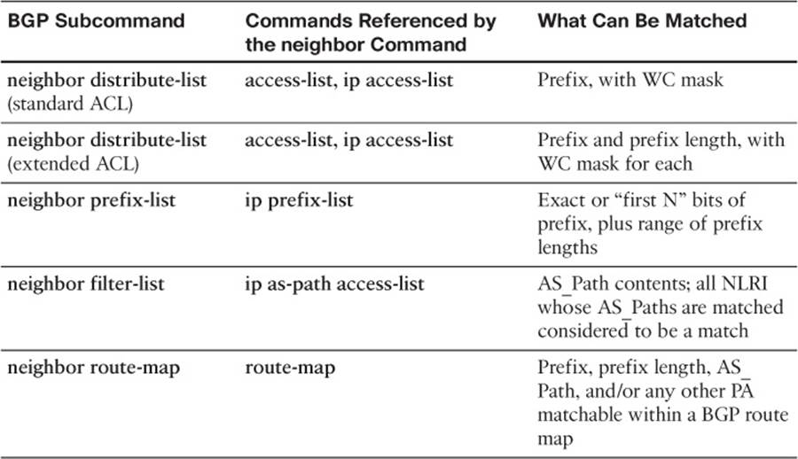
Table 14-2 BGP Filtering Tools
Inbound and Outbound BGP Filtering on Prefix/Length
Enterprises that choose to use BGP benefit from both learning routes from the connected ISPs and advertising the enterprise’s public prefix to the same ISPs. However, when the eBGP connections to the various ISPs come up, the enterprise BGP routers advertise all the best routes in each router’s BGP table over the eBGP connection. As a result, the ISPs could learn a best route that causes one ISP to send packets to the enterprise, with the enterprise then forwarding the packet out to another ISP. In such a case, the enterprise AS would be acting as a transit AS.
Enterprise engineers can, and probably should, make an effort to filter inappropriate routes sent to the ISP over the eBGP peer connections with the goal of preventing their enterprise AS from becoming a transit AS. Additionally, the enterprise can filter all private IP address ranges, in case any such address ranges get into the enterprise BGP router’s BGP table.
As an example, consider Figure 14-7, with the now-familiar prefix 192.135.250.0/28. As seen in earlier examples, both E1 and E2 learn this prefix, and both agree that the best route from ASN 11 (the enterprise) toward this prefix is through E2. The figure shows the BGP routing updates as dashed lines.
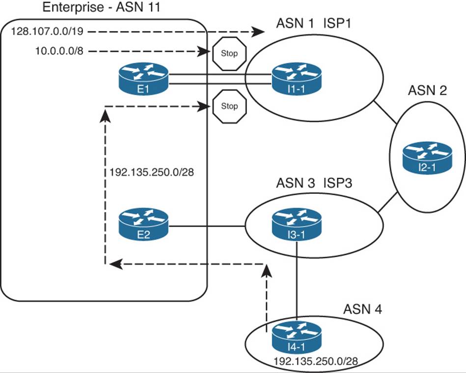
Figure 14-7 Need for Enterprise BGP Filtering
E1’s best route for 192.135.250.0/28 lists E2 as the next-hop router. So, without any filtering in place, E1 then advertises prefix 192.135.250.0/28 to Router I1-1 in ISP1. I1-1 can be configured to filter this prefix. (In the Chapter 13 examples, Router I1-1 was indeed configured to filter such prefixes.) However, if the enterprise did not filter this prefix when advertising to ISP1, and ISP1 did not filter it, ISP1 might choose the route through ASN 11 as its best route, making ASN 11 a transit AS for this prefix and consuming the enterprise’s Internet bandwidth.
Typically, an enterprise would use outbound filtering on its eBGP neighborships, filtering all routes except for the known public prefixes that need to be advertised into the Internet. Example 14-10 shows just such a case, using the neighbor prefix-list command. The example also highlights a particularly useful command, show ip bgp neighbor neighbor-ip advertised-routes, which shows the post-filter BGP update sent to the listed neighbor. The example shows the BGP Update before adding the filter, after adding the filter, and then after clearing the peer connection to router I1-1.
Example 14-10 Filtering to Allow Only Public Prefix 128.107.0.0/19 Outbound
! The next command occurs before filtering is added.
E1# show ip bgp neighbor 1.1.1.1 advertised-routes
BGP table version is 16, local router ID is 128.107.9.1
Status codes: s suppressed, d damped, h history, * valid, > best, i - internal,
r RIB-failure, S Stale
Origin codes: i - IGP, e - EGP, ? - incomplete
Network Next Hop Metric LocPrf Weight Path
*> 128.107.0.0/19 0.0.0.0 32768 i
*>i192.135.250.0/28 10.100.1.2 0 100 0 3 4 i
Total number of prefixes 2
! Next, the filtering is configured.
E1# configure terminal
Enter configuration commands, one per line. End with CNTL/Z.
E1(config)# ip prefix-list only-public permit 128.107.0.0/19
E1(config)# router bgp 11
E1(config-router)# neighbor 1.1.1.1 prefix-list only-public out
E1(config-router)# end
E1#
! Next, the Update sent to I1-1 is displayed.
E1# show ip bgp neighbor 1.1.1.1 advertised-routes
BGP table version is 16, local router ID is 128.107.9.1
Status codes: s suppressed, d damped, h history, * valid, > best, i - internal,
r RIB-failure, S Stale
Origin codes: i - IGP, e - EGP, ? - incomplete
Network Next Hop Metric LocPrf Weight Path
*> 128.107.0.0/19 0.0.0.0 32768 i
*>i192.135.250.0/28 10.100.1.2 0 100 0 3 4 i
Total number of prefixes 2
! Next, the peer connection is cleared, causing the filter to take effect.
E1# clear ip bgp 1.1.1.1
E1#
*Aug 17 20:19:51.763: %BGP-5-ADJCHANGE: neighbor 1.1.1.1 Down User reset
*Aug 17 20:19:52.763: %BGP-5-ADJCHANGE: neighbor 1.1.1.1 Up
! Finally, the Update is displayed with the filter now working.
E1# show ip bgp neighbor 1.1.1.1 advertised-routes
BGP table version is 31, local router ID is 128.107.9.1
Status codes: s suppressed, d damped, h history, * valid, > best, i - internal,
r RIB-failure, S Stale
Origin codes: i - IGP, e - EGP, ? - incomplete
Network Next Hop Metric LocPrf Weight Path
*> 128.107.0.0/19 0.0.0.0 32768 i
Total number of prefixes 1
Example 14-10 shows an interesting progression if you just read through the example from start to finish. To begin, the show ip bgp 1.1.1.1 advertised-routes command lists the routes that E1 has advertised to neighbor 1.1.1.1 (Router I1-1) in the past. Then, the configuration shows a prefix list that matches only 128.107.0.0/19, with a permit action; all other prefixes will be denied by the implied deny all at the end of each prefix list. Then, the neighbor 1.1.1.1 prefix-list only-public out BGP subcommand tells BGP to apply the prefix list to filter outbound routes sent to I1-1.
The second part of the output shows an example of how BGP operates on a Cisco router, particularly how BGP requires that the neighbor be cleared before the newly configured filter takes effect. Router E1 has already advertised two prefixes to this neighbor: 128.107.0.0/19 and 192.135.250.0/28, as seen at the beginning of the example. To make the filtering action take effect, the router must be told to clear the neighborship with Router I1-1. The clear ip bgp 1.1.1.1 command tells E1 to perform a hard reset of that neighbor connection, which brings down the TCP connection and removes all BGP table entries associated with that neighbor. The neighbor (I1-1, using address 1.1.1.1) also removes its BGP table entries associated with Router E1. After the neighborship recovers, E1 resends its BGP Update to Router I1-1—but this time with one less prefix, as noted at the end of the example with the output of the show ip bgp neighbor 1.1.1.1 advertised-routes command.
This same filtering action could have been performed with several other configuration options: using the neighbor distribute-list or neighbor route-map commands. The neighbor distribute-list command refers to an IP ACL, which tells Cisco IOS to filter routes based on matching the prefix (standard ACL) or prefix/length (extended ACL). The neighbor route-map command refers to a route map that can use several matching options to filter routes, keeping routes matched with a route map permit clause and filtering routes matched with a route map deny clause. Example 14-11 shows two such options just for comparison’s sake.
Example 14-11 Alternatives to the Configuration in Example 14-10
! First option – ACL 101 as a distribute-list
access-list 101 permit ip host 128.107.0.0 host 255.255.224.0
router bgp 11
neighbor 1.1.1.1 distribute-list 101 out
! Second option: Same prefix list as Example 14-10, referenced by a route map
ip prefix-list only-public seq 5 permit 128.107.0.0/19
!
route-map only-public-rmap permit 10
match ip address prefix-list only-public
!
router bgp 11
neighbor 1.1.1.1 route-map only-public-rmap out
Clearing BGP Neighbors
As noted in Example 14-10 and the related explanations, Cisco IOS does not cause a newly configured BGP filter to take effect until the neighbor relationship is cleared. The neighborship can be cleared in several ways, including reloading the router and by administratively disabling and reenabling the BGP neighborship using the neighbor shutdown and no neighbor shutdown configuration commands. However, Cisco IOS supports several options on the clear ip bgp EXEC command for the specific purpose of resetting BGP connections. This section examines the differences in these options.
Each variation on the clear ip bgp... command either performs a hard reset or soft reset of one or more BGP neighborships. When a hard reset occurs, the local router brings down the neighborship, brings down the underlying TCP connection, and removes all BGP table entries learned from that neighbor. Both the local and neighboring router react just like they do for any failed BGP neighborship by removing their BGP table entries learned over that neighborship. With a soft reset, the router does not bring down the BGP neighborship or the underlying TCP connection. However, the local router resends outgoing Updates, adjusted per the outbound filter, and reprocesses incoming Updates per the inbound filter, which adjusts the BGP tables based on the then-current configuration.
Table 14-3 lists many of the variations on the clear ip bgp command, with a reference as to whether it uses hard or soft reset.
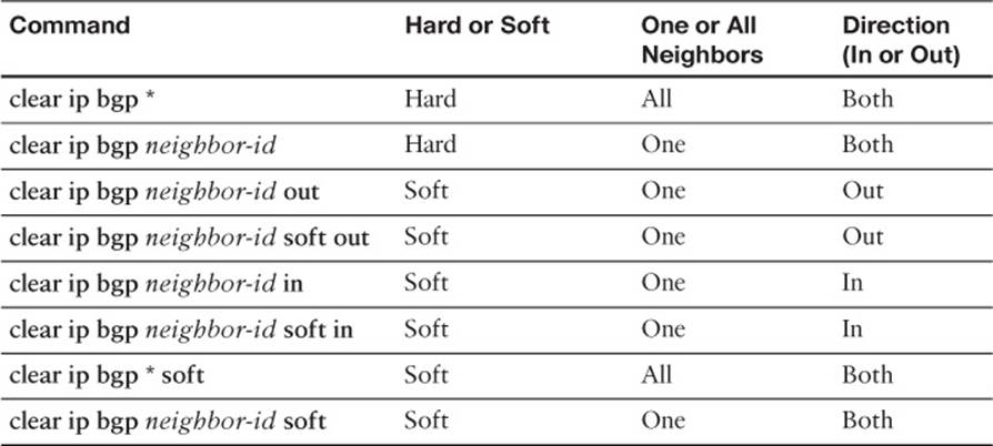
Table 14-3 BGP clear Command Options
The commands listed in the table should be considered as pairs. In the first pair, both commands perform a hard reset. The first command uses a * instead of the neighbor IP address, causing a hard reset of all BGP neighbors, while the second command resets that particular neighbor.
The second pair of commands performs soft resets for a particular neighbor but only for outgoing updates, making these commands useful when a router changes its outbound BGP filters. Both commands do the same function; two such commands exist in part because of the history of BGP’s implementation in Cisco IOS. When issued, these two commands cause the router to reevaluate its existing BGP table and create a new BGP Update for that neighbor. The router builds that new Update based on the existing configuration, so any new or changed outbound filters affect the contents of the Update. The router sends the new BGP Update, and the neighboring router receives the new Update and adjusts its BGP table as a result.
The third pair of commands performs soft resets for a particular neighbor, but only for incoming updates, making these commands useful when a router changes its inbound BGP filters. However, unlike the two previous commands in the table, these two commands do have slightly different behavior and need a little more description.
The clear ip bgp neighbor-id soft in command, the older command of the two, works only if the configuration includes the neighbor neighbor-id soft-reconfiguration inbound BGP configuration command for this same neighbor. This configuration command causes the router to retain the received BGP Updates from that neighbor. This consumes extra memory on the router, but it gives the router a copy of the original pre-filter Update received from that neighbor. Using that information, the clear ip bgp neighbor-id soft in command tells Cisco IOS to reapply the inbound filter to the cached received Update, updating the local router’s BGP table.
The newer version of the clear ip bgp command, namely, the clear ip bgp neighbor-id in command (without the soft keyword), removes the requirement for the neighbor neighbor-id soft-reconfiguration inbound configuration command. Instead, the router uses a newer BGP feature, the route refresh feature, which essentially allows a BGP router to ask its neighbor to resend its full BGP Update. The clear ip bgp neighbor-id in command tells the local router to use the route refresh feature to ask the neighbor to resend its BGP Update, and then the local router can apply its current inbound BGP filters, updating its BGP table.
Example 14-12 shows a sample of how to confirm whether a router has the route refresh capability. In this case, both the local router (E1 from Figure 14-5) and the neighbor (I1-1 from Figure 14-5) have route refresh capability. As a result, E1 can perform a soft reset inbound without the need to consume the extra memory with the neighbor soft-reconfiguration inbound configuration command.
Example 14-12 Alternatives to the Configuration in Example 14-10
E1# show ip bgp neighbor 1.1.1.1
BGP neighbor is 1.1.1.1, remote AS 1, external link
BGP version 4, remote router ID 1.1.1.1
BGP state = Established, up for 00:04:21
Last read 00:00:20, last write 00:00:48, hold time is 180, keepalive interval is
60 seconds
Neighbor capabilities:
Route refresh: advertised and received(new)
! Lines omitted for brevity
The last pair of commands in Table 14-3 do a soft reset both inbound and outbound at the same time, either for all neighbors (the * option) or for the single neighbor listed in the clear command.
Displaying the Results of BGP Filtering
To verify and troubleshoot filtering configurations, you need to see both the results before and after the filter. Cisco IOS provides several show commands that allow you to do exactly that. For example, Example 14-10 shows several cases of the show ip bgp neighbor advertised-routescommand that shows the post-filter BGP Updates sent by a router. Figure 14-8 summarizes these commands, showing how they can be used to display the pre- and post-filter BGP table contents. The figure shows Router E1, with inbound filtering for Updates received from Router I3-1 and outbound filtering of BGP Updates sent to Router I1-1.
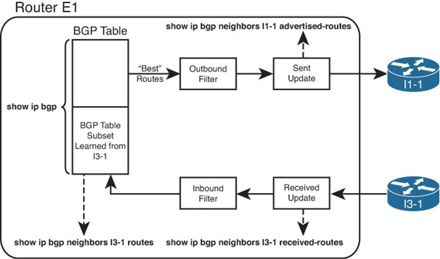
Figure 14-8 show Commands Related to BGP Filtering
The commands for displaying inbound updates, at the bottom of the figure, display output in the same format as the show ip bgp command. These commands restrict the contents to either exactly what has been received from that one neighbor (the show ip bgp neighbors received-routescommand) or what has been received and passed through any inbound filter (the show ip bgp neighbors routes command).
One of the two commands helpful for the inbound direction, namely, the show ip bgp neighbor received-routes command, requires the configuration of the BGP subcommand neighbor soft-reconfiguration inbound. As a result, to see the pre-filter BGP Update received from a neighbor, a router must configure this extra command, which causes the router to use more memory to store the inbound Update. However, when learning in a lab, the extra memory should not pose a problem.
Of the two commands for outbound filtering, the post-filter command is somewhat obvious, but there is no command to specifically display a pre-filter view of the BGP Update sent to a neighbor. However, BGP advertises the best route for each prefix in the BGP table, within certain restrictions. Those restrictions state that BGP will not advertise iBGP-learned routes to an iBGP peer, and a router will not advertise the best route back to the same neighbor that advertised that route. So, to see the pre-filter BGP table entries, use the show ip bgp command, look for all the best routes, and then consider the additional rules. Use the show ip bgp neighbor advertised-routes command to display the post-filter BGP Update for a given neighbor.
Example 14-13 shows the output of these commands on E1. In this case, E1 has already been configured with an inbound filter that filters inbound prefixes 184.0.0.0/8 and 185.0.0.0/8. (The filter configuration is not shown.) As a result, the post-filter output lists five prefixes, and the pre-filter output lists seven prefixes. The example also shows the error message when soft reconfiguration is not configured.
Example 14-13 Displaying the BGP Table Pre- and Post-Inbound Filter
E1# show ip bgp neighbors 1.1.1.1 routes
BGP table version is 78, local router ID is 11.11.11.11
Status codes: s suppressed, d damped, h history, * valid, > best, i - internal,
r RIB-failure, S Stale
Origin codes: i - IGP, e - EGP, ? - incomplete
Network Next Hop Metric LocPrf Weight Path
*> 0.0.0.0 1.1.1.1 0 0 1 i
*> 181.0.0.0/8 1.1.1.1 0 1 2 111 111 i
*> 182.0.0.0/8 1.1.1.1 0 1 2 222 i
*> 183.0.0.0/8 1.1.1.1 0 1 2 i
* 192.135.250.0/28 1.1.1.1 0 1 2 3 4 i
Total number of prefixes 5
E1# show ip bgp neighbors 1.1.1.1 received-routes
% Inbound soft reconfiguration not enabled on 1.1.1.1
E1# configure terminal
Enter configuration commands, one per line. End with CNTL/Z.
E1(config)# router bgp 11
E1(config-router)# neighbor 1.1.1.1 soft-reconfiguration inbound
E1(config-router)# end
E1#
E1# show ip bgp neighbors 1.1.1.1 received-routes
BGP table version is 78, local router ID is 11.11.11.11
Status codes: s suppressed, d damped, h history, * valid, > best, i - internal,
r RIB-failure, S Stale
Origin codes: i - IGP, e - EGP, ? - incomplete
Network Next Hop Metric LocPrf Weight Path
*> 0.0.0.0 1.1.1.1 0 0 1 i
*> 181.0.0.0/8 1.1.1.1 0 1 2 111 111 i
*> 182.0.0.0/8 1.1.1.1 0 1 2 222 i
*> 183.0.0.0/8 1.1.1.1 0 1 2 i
*> 184.0.0.0/8 1.1.1.1 0 1 2 i
*> 185.0.0.0/8 1.1.1.1 0 1 2 i
* 192.135.250.0/28 1.1.1.1 0 1 2 3 4 i
Total number of prefixes 7
Peer Groups
Cisco IOS creates BGP updates, by default, on a neighbor-by-neighbor basis. As a result, more neighbors result in more CPU resources being used. Also, by applying nondefault settings (for example, performing filtering using prefix lists, route maps, or filter lists) to those neighbors, even more CPU resources are required.
However, many neighbors might have similarly configured parameters. Cisco IOS allows you to logically group those similar neighbors into a BGP peer group. Then, you can apply your nondefault BGP configuration to the peer group, as opposed to applying those parameters to each neighbor individually. In fact, a single router can have multiple peer groups, each representing a separate set of parameters. The result can be a dramatic decrease in required CPU resources.
Note
Even though the filtering operations are performed for a peer group, rather than the individual members of the peer group, a Cisco IOS router still sends out individual BGP Updates to each of its neighbors. This is a requirement, based on BGP’s characteristic of establishing a TCP session with each neighbor.
To illustrate the configuration of a peer group, consider Figure 14-9. In the figure, the HQ router has connections to two ISPs. Because the same IP prefix list needs to be applied to each peer, a BGP peer group is used in the configuration, as shown in Example 14-14.
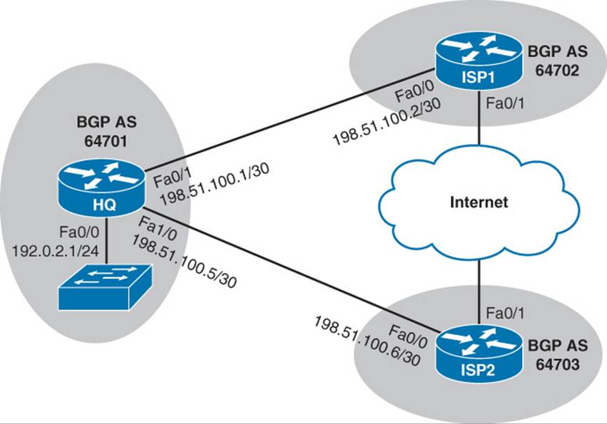
Figure 14-9 Topology Using a BGP Peer Group
Example 14-14 BGP Peer Group Configuration
router bgp 64701
bgp log-neighbor-changes
network 192.0.2.0
network 198.51.100.0 mask 255.255.255.252
network 198.51.100.4 mask 255.255.255.252
neighbor ROUTE-PG peer-group
neighbor ROUTE-PG prefix-list ROUTE-DEMO in
neighbor 198.51.100.2 remote-as 64702
neighbor 198.51.100.2 peer-group ROUTE-PG
neighbor 198.51.100.6 remote-as 64703
neighbor 198.51.100.6 peer-group ROUTE-PG
!
ip prefix-list ROUTE-DEMO seq 5 deny 10.0.0.0/8 le 32
ip prefix-list ROUTE-DEMO seq 10 deny 172.16.0.0/12 le 32
ip prefix-list ROUTE-DEMO seq 15 deny 192.168.0.0/16 le 32
ip prefix-list ROUTE-DEMO seq 20 permit 0.0.0.0/0
ip prefix-list ROUTE-DEMO seq 25 permit 0.0.0.0/0 ge 8
The purpose of Example 14-14 is to prevent RFC 1918 private IP addresses from being learned by Router HQ. The neighbor ROUTE-PG peer-group command creates a BGP peer group named ROUTE-PG. The neighbor ROUTE-PG prefix-list ROUTE-DEMO in command applies theROUTE-DEMO IP prefix list, in the inbound direction, to the peer group. Also, the commands neighbor 198.51.100.2 peer-group ROUTE-PG and neighbor 198.51.100.6 peer-group ROUTE-PG make ISP1 (198.51.100.2) and ISP2 (198.51.100.6) members of the peer group.
BGP Path Attributes and Best-Path Algorithm
BGP supports a wide variety of Path Attributes (PA). Some of the PAs exist solely to be used as part of the litany of options in the BGP best-path algorithm, some have nothing to do with the BGP best-path algorithm, and some impact the best-path algorithm as well as being used for other purposes. For example, the Local Preference PA exists to give control to a single AS regarding its outbound routes from an AS-wide perspective. Conversely, the BGP Next_Hop PA provides BGP with a place to list the next-hop IP address for a path, but it does not provide a useful means for engineers to set different values for the purpose of influencing the best-path choice.
The term BGP best-path algorithm refers to the process by which BGP on a single router examines the competing BGP paths (routes) in its BGP table, for a single prefix, choosing one route as the best route. The best path algorithm has many steps, but it eventually results in the choice of a single route for each prefix as that router’s best BGP path.
This section of the chapter examines the BGP PAs used by the BGP best-path algorithm, the BGP best-path algorithm itself, and some related topics.
BGP Path Attributes
BGP Path Attributes define facts about a particular route or path through a network. Each PA defines something different about the path, so to truly understand BGP PAs, you need to examine each PA. This section begins by reviewing a few PAs that should now be familiar, and then this section introduces a few new PAs.
BGP uses the Autonomous System Path (AS_Path) PA for several purposes. This particular PA lists the ASNs in the end-to-end path. BGP uses the AS_Path PA as its primary loop-prevention tool. Specifically, when an eBGP peer receives an Update, if its own ASN is already in the received AS_Path, that route has already been advertised into the local ASN and should be ignored. In addition to loop prevention, the BGP best-path algorithm uses the AS_Path PA to calculate the AS_Path length, which the algorithm considers as one of its many steps.
BGP also defines the next-hop IP address (Next_Hop) of a route as a PA. BGP can advertise one of several different IP addresses as a route’s Next_Hop, depending on several factors. To support such features, BGP needs to list the Next_Hop IP address for each path (route), and BGP defines this concept in the Next_Hop PA. The best-path algorithm includes a check related to the Next_Hop IP address of the route.
Table 14-4 lists these two PAs, plus a few more PAs, and a related BGP feature (Weight) that is not a PA but is used by Cisco BGP best-path implementation. The table lists the PAs in the same order that the BGP best-path algorithm will consider them. The table also describes each feature listed in the table, relative to whether it is most useful to influence outbound routes (away from the enterprise) and inbound routes (toward the enterprise).
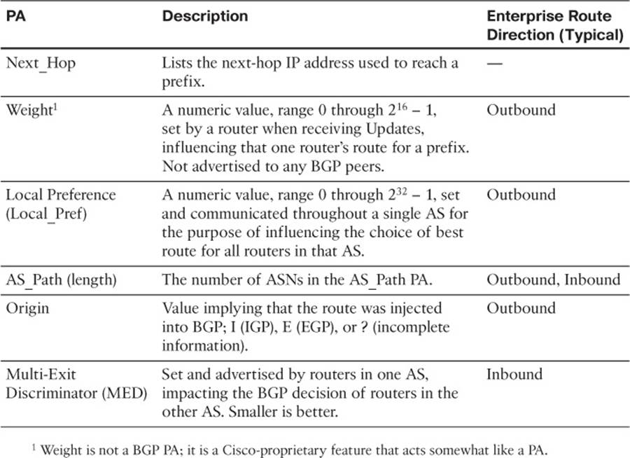
Table 14-4 BGP Path Attributes That Affect the BGP Best-Path Algorithm
The short descriptions in the table can be helpful for review when doing your final preparation study, but the table does not hold enough information to truly appreciate how an engineer might use these PAs effectively. The next two major sections of this chapter examine most of these PAs and describe how to influence the best-path choice with each.
To find the current settings of the features in Table 14-4, you can use commands like show ip bgp and show ip bgp prefix/length. However, picking the values out of the clutter in the output of the show ip bgp command can be a challenge. Figure 14-10 shows a sample of this command’s output and some notations on where to find the various PA settings.
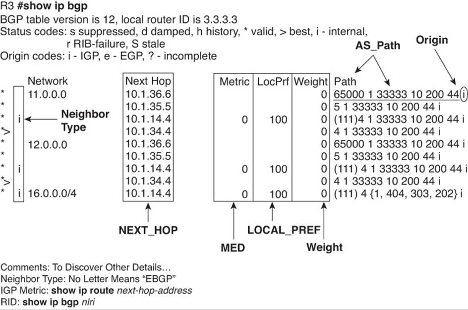
Figure 14-10 Finding PA Settings in the Output of the show ip bgp Command
The examples throughout the rest this chapter include examples of these commands, along with the PA settings as changed by various route maps.
Overview of the BGP Best-Path Algorithm
The BGP best-path algorithm follows the steps shown in shorthand form in Table 14-5. The table lists steps 0 through 8, a short descriptive phrase, and a notation about the criteria for one value to be better than another.
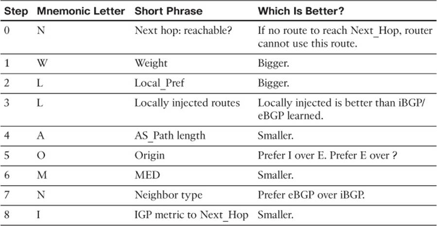
Table 14-5 BGP Decision Process Plus Mnemonic: N WLLA OMNI
Note
The step numbering of the BGP best-path steps does not exist in the BGP RFCs. The steps are numbered in this book for easier reference. Because the RFCs do not dictate a particular step numbering, other references likely use different step numbers. Therefore, do not be concerned about memorizing the step numbers.
Starting with a Step 0 might seem odd, but it helps make an important point about the logic listed at this step. Some BGP best-path references include the logic in this step as a best-path step, and some just list this same information as a side note. Regardless, the Step 0 concept is important. For Step 0, a router looks at the BGP route and compares the Next_Hop IP address to the IP routing table.
If that router does not have a matching IP route for the BGP route’s Next_Hop IP address, that router will not know how to forward packets for that particular prefix, using that particular route. To avoid using such a route, at Step 0, the BGP best-path algorithm removes such routes from consideration. BGP then uses the following eight steps, in order, until one best route is chosen for a given prefix.
If a router still did not determine a best route when finishing Step 8, the router takes several other small steps to break the tie. At this point, the competing routes are considered to be just as good as each other. However, unlike IGPs, BGP needs to choose one and only one route as best, in part because BGP advertises only the best routes to its neighbors. In such cases, BGP breaks the tie with these additional steps, which would be considered Steps 9–11:
Step 9. Oldest (longest-known) eBGP route
Step 10. Lowest neighbor BGP RID
Step 11. Lowest neighbor IP address
Taking a more detailed view of the entire best-path algorithm, BGP begins by choosing the oldest known route for a given prefix as the best route. It then takes the next longest-known route for that same prefix and compares the two routes using the best-path algorithm. The router eventually chooses one of the two BGP routes as the best path (route). If another route exists for the same prefix, the router repeats the process, using the winner of the previous comparisons and the new route, choosing one of those as the better route. The process continues until all routes have been considered, with one route being listed as best in the BGP table.
For example, if Router R1 were considering two routes for prefix 181.0.0.0/8, it would first make sure that both routes had reachable Next_Hop IP addresses. The router would then compare the Weight settings, choosing the route with the bigger Weight. If they tied on Weight, the router would prefer the route with a bigger Local_Pref. If again a tie, the router would prefer the one route that was injected into BGP locally (using the network command or using route redistribution). If neither or both routes were locally injected, the router moves on to AS_Path length, and so on, until the router chooses one of the two as the better route.
As soon as one of the steps determines a best route, the comparison of those two routes stops.
Perspectives on the Core Eight Best-Path Steps
Some of the BGP best-path steps purposefully give the engineer a tool for influencing the choice of best path, whereas other steps have a different purpose, often simply being a side effect of some BGP feature. So, when an engineer starts building a BGP implementation plan, only a subset of the core eight BGP best-path steps need be considered, as follows:
![]() Weight (Step 1)
Weight (Step 1)
![]() Local_Pref (Step 2)
Local_Pref (Step 2)
![]() AS_Path Length (Step 4)
AS_Path Length (Step 4)
![]() MED (often called metric) (Step 6)
MED (often called metric) (Step 6)
Because the ROUTE exam focuses on the more practical aspects of BGP for enterprises, it gives much more attention to these four features and less attention to the other BGP best-path steps. This chapter describes each of these four features in some depth in the context of best-path selection. However, before focusing on these four items, it can be helpful to see a small glimpse into the meaning of the other steps, which can be helpful as you work to memorize the steps in the BGP best-path algorithm.
Step 3 compares the source from which the routes were added to the BGP table. When the BGP best-path algorithm compares two routes at this step, if one were injected into BGP locally and the other were not (it was learned from a BGP peer), the router chooses the route that was injected locally. The Chapter 13 section “Injecting Routes into BGP for Advertisement to the ISPs” describes the two ways to locally inject these routes, the network command, and redistribution from an IGP.
Step 5 refers to the BGP Origin PA. The Origin PA attempts to identify the source from outside BGP from which the route was injected into BGP. The three Origin code values are
![]() i: Injected from an IGP (using a network command)
i: Injected from an IGP (using a network command)
![]() e: Injected from exterior gateway protocol (EGP)
e: Injected from exterior gateway protocol (EGP)
![]() ?: Undetermined
?: Undetermined
Although the original intent of the Origin PA is to identify the source from which BGP learned the route, routers can also set the Origin PA as part of a strategy to influence the BGP best path.
Step 7 refers to the Neighbor type: iBGP or eBGP. Remembering that BGP compares two routes at a time, if one is learned with eBGP and the other with iBGP, the router chooses the eBGP route as best. Using this feature to influence the best-path choice would be difficult, because the ASN in which a router resides is fixed by the BGP design.
Finally, Step 8 refers to the IGP metric to the Next_Hop address. At this step, the router compares the metrics of the IP routes for each Next_Hop IP address and chooses the BGP route with the lower IGP metric to its Next_Hop. (If an IGP-learned route is not used—for example, if both use connected routes—BGP considers the metrics to tie.) It is conceivable that an engineer might tune the IGP to manipulate BGP’s best-path choice, but this step is so far into the algorithm that the earlier and more flexible settings would be much better options.
Memorization Tips for BGP Best Path
This short section suggests a mnemonic tool to help you memorize Steps 0 through 8 of the BGP best-path algorithm. Feel free to skim this section for now, or ignore it entirely—there is no requirement that you memorize the best-path algorithm using the mnemonics in this section. (However, you might want to at least review upcoming Figure 14-11, which gives a good visual reference for some of the information summarized in Table 14-5.) But you should plan on memorizing the list at some point before the exam, even if you ignore the mnemonic device.
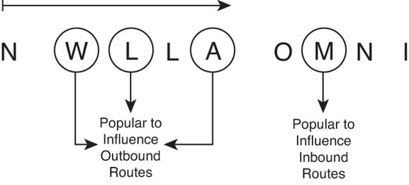
Figure 14-11 BGP Best-Path Mnemonics
First, if you refer back to the BGP best-path algorithm as listed in Table 14-5, you see that the second column lists a single-letter mnemonic letter. These letters match the first letter of the description in the third column of that table. Then, take these initial letters and group them as follows:
![]() N
N
![]() WLLA
WLLA
![]() OMNI
OMNI
The N is listed separately, because it represents the “Is the next-hop reachable?” logic of Step 0 and is somewhat separate from the other steps.
The mnemonic groups the eight main steps as two sets of four letters for a couple of reasons. Both sets can be pronounced, even if they don’t spell words. It should be easier to memorize as two sets of four. And maybe most importantly, the first set of four letters, representing Steps 1 through 4, include all the features that engineers typically use to influence outbound routes from the enterprise:
![]() WLLA: Refers to the three steps that an engineer might use to influence outbound routes: Weight, Local_Pref, and AS_Path length. (Additionally, the second L, in WLLA for Step 3, represents the “Locally injected routes” choice.)
WLLA: Refers to the three steps that an engineer might use to influence outbound routes: Weight, Local_Pref, and AS_Path length. (Additionally, the second L, in WLLA for Step 3, represents the “Locally injected routes” choice.)
![]() OMNI: As listed in Table 14-5, the letters represent Origin (i, e, or ?), MED, neighbor type (eBGP over iBGP), and IGP metric to Next_Hop.
OMNI: As listed in Table 14-5, the letters represent Origin (i, e, or ?), MED, neighbor type (eBGP over iBGP), and IGP metric to Next_Hop.
So, if you can memorize N WLLA OMNI, by the time you’ve read this chapter, you can probably pick out which of those correlate to the four bigger topics later in this chapter: Weight, Local_Pref, AS_Path length, and MED. Hopefully with a little more study, you can memorize the rest of the list.
Figure 14-11 shows the mnemonic letters in graphical form just as another aid in memorizing the steps. It also shows a reminder of which features are most likely to be used to influence outbound routes from the enterprise, and the one setting (MED) most likely to be used to influence inbound routes into the enterprise.
The rest of this chapter focuses on a deeper explanation of the four best-path steps that engineers typically use to influence the choice of best path.
Influencing an Enterprise’s Outbound Routes
This section examines three different features that can influence the outbound routes from an enterprise: Weight, the Local_Pref PA, and AS_Path length. The topics are listed in the order used by the BGP best-path algorithm (Steps 1, 2, and 4). It also introduces the concept of a Routing Table Manager (RTM) function on a router.
Influencing BGP Weight
A Cisco router can use the BGP Weight, on that single router, to influence that one router’s choice of outbound route. To do so, when a router receives a BGP Update, that router can set the Weight either selectively, per route, using a route map, or for all routes learned from a single neighbor. The router’s best-path algorithm then examines the Weight of competing routes, choosing the route with the bigger Weight.
The Cisco-proprietary Weight settings configured on a single router can influence only that one router, because the Weight cannot be communicated to other neighboring BGP routers. So, to use the Weight, a router must be configured to examine incoming Updates to set the Weight. The Weight cannot simply be learned in a received Update, because that Update message does not support a field in which to communicate the Weight setting.
Table 14-6 summarizes some of the key facts about BGP administrative Weight. Following the table, the text first explains a sample internetwork and its existing configuration, a configuration that begins with configurations that do not set any values that influence the choice of best paths. The next section shows how to set the Weight using the neighbor route-map in command, which allows a router to set different Weights for different routes. The second example shows how to set the Weight for all routes learned from a neighbor, using the neighbor weight command.
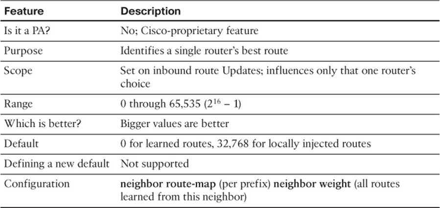
Table 14-6 Key Features of Administrative Weight
Note
For those of you memorizing using the N WLLA OMNI mnemonic, Weight is the W in WLLA.
Sample Internetwork Used in the Weight Examples
Figure 14-12 shows a sample internetwork used to demonstrate setting the Weight. The figure shows a single enterprise and a single enterprise router. The following design requirements have already been met by the configuration in Router E1 and in the ISP routers:
![]() E1 and I1-1 use loopback IP addresses (11.11.11.11 and 1.1.1.1) for their neighborship.
E1 and I1-1 use loopback IP addresses (11.11.11.11 and 1.1.1.1) for their neighborship.
![]() E1 and I3-1 use interface IP addresses for their neighborship.
E1 and I3-1 use interface IP addresses for their neighborship.
![]() None of the routers have attempted to change any settings that can impact the choice of best path.
None of the routers have attempted to change any settings that can impact the choice of best path.
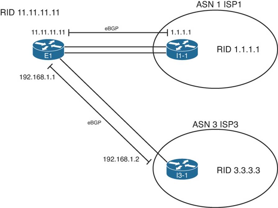
Figure 14-12 Sample Internetwork for BGP Weight Examples
Next, to have some routes to manipulate with the upcoming examples, the ISP routers each advertise BGP routes for the same five prefixes. Figure 14-13 shows five such prefixes that both ISPs advertise to E1.
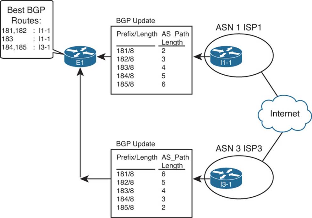
Figure 14-13 Prefixes and AS_Path Lengths Used in Upcoming Examples
Just to get a little deeper understanding of the best-path algorithm before getting into the Weight configuration, consider the original configuration state of the sample internetwork, with no attempt to influence E1’s choice of best path. The best path for four of the five prefixes will be obvious. Prefixes 181.0.0.0/8 and 182.0.0.0/8 have a shorter AS_Path through ISP1, and 184.0.0.0/8 and 185.0.0.08 have a shorter AS_Path through ISP3. Only 183.0.0.0/8 is in question, because its AS_Path length for the competing routes is equal. Example 14-15 shows the output of the show ip bgp 176.0.0.0/4 longer-prefixes command, which lists all five of the BGP prefixes listed in Figure 14-13, confirming the results. (Prefix 176.0.0.0/4 implies a range of values whose first octets are in the range 176 through 191, which includes the routes listed in Example 14-15.)
Example 14-15 BGP Configuration on E1: Neighborships Configured
E1# show ip bgp 176.0.0.0/4 longer-prefixes
BGP table version is 41, local router ID is 128.107.9.1
Status codes: s suppressed, d damped, h history, * valid, > best, i - internal,
r RIB-failure, S Stale
Origin codes: i - IGP, e - EGP, ? - incomplete
Network Next Hop Metric LocPrf Weight Path
* 181.0.0.0/8 192.168.1.2 0 0 3 2 50 51 52 1811 i
*> 1.1.1.1 0 0 1 1811 i
* 182.0.0.0/8 192.168.1.2 0 0 3 2 50 51 1822 i
*> 1.1.1.1 0 0 1 2 1822 i
* 183.0.0.0/8 192.168.1.2 0 0 3 2 50 1833 i
*> 1.1.1.1 0 0 1 2 50 1833 i
*> 184.0.0.0/8 192.168.1.2 0 0 3 2 1844 i
* 1.1.1.1 0 0 1 2 50 51 1844 i
*> 185.0.0.0/8 192.168.1.2 0 0 3 1855 i
* 1.1.1.1 0 0 1 2 50 51 52 1855 i
First, consider the best-path algorithm on Router E1 for 181.0.0.0/8. E1 knows two BGP routes for 181.0.0.0/8, as expected. The one listed as the best path has 1.1.1.1 (I1-1) as Next_Hop. The following list outlines the best-path logic:
Step 0. The Next_Hop of each is reachable. (Otherwise the neighbors would not be up.)
Step 1. The Weight ties (both 0).
Step 2. The Local_Pref ties (unset, so no value is listed; defaults to 100).
Step 3. Neither route is locally injected; both are learned using BGP, so neither is better at this step.
Step 4. AS_Path length is shorter for the route through I1-1 (1.1.1.1).
Next, consider the example of the route to 183.0.0.0/8. E1 currently lists the path through I1-1 (1.1.1.1) as best, but the best-path decision actually falls all the way to Step 9. For completeness’ sake, E1’s best-path logic runs as follows:
Step 0. The Next_Hop of each is reachable. (Otherwise the neighbors would not be up.)
Step 1. The Weight ties (both 0).
Step 2. The Local_Pref ties (unset, defaults to 100).
Step 3. Neither route is locally injected.
Step 4. AS_Path length is 4 in both cases.
Step 5. Both Origin codes are i.
Step 6. MED, listed under the Metric column, ties (0).
Step 7. Neighbor type for each neighbor is eBGP.
Step 8. IGP metric does not apply, because neither uses IGP routes. (The routes from E1 to 1.1.1.1 are static routes.)
Step 9. The route learned from 1.1.1.1 is the oldest route.
Although you might believe the claims at Step 9, the output in Example 14-15 does not explicitly state that fact. However, when Cisco IOS lists output in the variations of the show ip bgp command, the oldest route for each prefix is listed last, and the newest (most recently learned) is listed first. Example 14-16 confirms this logic, and confirms how Step 9 works in this case. Example 14-16 clears peer 1.1.1.1 (I1-1), making E1’s route through 192.168.1.2 (I3-1) become the oldest known route for 183.0.0.0/8.
Example 14-16 Clearing Neighbors to Force a New Route
E1# clear ip bgp 1.1.1.1
E1#
*Aug 24 11:30:41.775: %BGP-5-ADJCHANGE: neighbor 1.1.1.1 Down User reset
*Aug 24 11:30:43.231: %BGP-5-ADJCHANGE: neighbor 1.1.1.1 Up
E1# show ip bgp 176.0.0.0/4 longer-prefixes
BGP table version is 47, local router ID is 128.107.9.1
Status codes: s suppressed, d damped, h history, * valid, > best, i - internal,
-r RIB-failure, S Stale
Origin codes: i - IGP, e - EGP, ? - incomplete
Network Next Hop Metric LocPrf Weight Path
*> 181.0.0.0/8 1.1.1.1 0 0 1 1811 i
* 192.168.1.2 0 0 3 2 50 51 52 1811 i
*> 182.0.0.0/8 1.1.1.1 0 0 1 2 1822 i
* 192.168.1.2 0 0 3 2 50 51 1822 i
* 183.0.0.0/8 1.1.1.1 0 0 1 2 50 1833 i
*> 192.168.1.2 0 0 3 2 50 1833 i
* 184.0.0.0/8 1.1.1.1 0 0 1 2 50 51 1844 i
*> 192.168.1.2 0 0 3 2 1844 i
* 185.0.0.0/8 1.1.1.1 0 0 1 2 50 51 52 1855 i
*> 192.168.1.2 0 0 3 1855 i
After the hard reset of peer 1.1.1.1, E1’s oldest-known route for 183.0.0.0/8 is the route through 192.168.1.2, listed second (last). That E1 now chooses this route as best is another confirmation that E1’s best-path decision fell to Step 9.
Setting the BGP Administrative Weight Using a Route Map
The neighbor neighbor-ip route-map in BGP subcommand tells a router to apply the route map to all BGP Updates received from the listed neighbor. Such route maps always attempt to filter routes. The router allows routes first matched in a permit clause and filters (discards) routes first matched with a deny clause.
BGP route maps can also be used to change the PAs of routes by using the set command. For example, a router could use a neighbor 1.1.1.1 route-map fred in command. The route map could contain permit clauses that cause some routes to not be filtered. In those same route map clauses, the inclusion of commands such as set weight 100 and set local-preference 200 can be used to set items such as the Weight or Local_Pref of a route. (Although you can configure a set command in a route map deny clause, the set command has no effect, because the deny clause filters the route.)
Example 14-17 shows a sample configuration that sets the Weight for prefix 181.0.0.0/8 as learned from I3-1 (neighbor ID 192.168.1.2). As shown in Example 14-15, E1’s original best route for this prefix is through I1-1 (1.1.1.1), because of the shorter AS_Path length at Step 4 of the best-path algorithm. By setting the Weight higher on the route learned from I3-1, E1 now chooses the route through I3-1.
Example 14-17 Setting the Weight to 50 for 181/8, as Learned from I3-1
E1# conf t
Enter configuration commands, one per line. End with CNTL/Z.
E1(config)# ip prefix-list match-181 permit 181.0.0.0/8
E1(config)# route-map set-weight-50 permit 10
E1(config-route-map)# match ip address prefix-list match-181
E1(config-route-map)# set weight 50
E1(config-route-map)# route-map set-weight-50 permit 20
E1(config-route-map)# router bgp 11
E1(config-router)# neighbor 192.168.1.2 route-map set-weight-50 in
E1(config-router)# end
E1#
E1# clear ip bgp 192.168.1.2 soft
E1# show ip bgp 176.0.0.0/4 longer-prefixes
BGP table version is 48, local router ID is 128.107.9.1
Status codes: s suppressed, d damped, h history, * valid, > best, i - internal,
r RIB-failure, S Stale
Origin codes: i - IGP, e - EGP, ? - incomplete
Network Next Hop Metric LocPrf Weight Path
* 181.0.0.0/8 1.1.1.1 0 0 1 1811 i
*> 192.168.1.2 0 50 3 2 50 51 52 1811 i
*> 182.0.0.0/8 1.1.1.1 0 0 1 2 1822 i
* 192.168.1.2 0 0 3 2 50 51 1822 i
* 183.0.0.0/8 1.1.1.1 0 0 1 2 50 1833 i
*> 192.168.1.2 0 0 3 2 50 1833 i
* 184.0.0.0/8 1.1.1.1 0 0 1 2 50 51 1844 i
*> 192.168.1.2 0 0 3 2 1844 i
* 185.0.0.0/8 1.1.1.1 0 0 1 2 50 51 52 1855 i
*> 192.168.1.2 0 0 3 1855 i
! The next command lists the pre-route-map received Update
E1# show ip bgp neigh 192.168.1.2 received-routes | include 181
* 181.0.0.0/8 192.168.1.2 0 0 3 2 50 51 52 1811 i
! The next command shows the post-route-map received Update
E1# show ip bgp neigh 192.168.1.2 routes | incl 181
*> 181.0.0.0/8 192.168.1.2 0 50 3 2 50 51 52 1811 i
The configuration uses a single-line IP prefix list that matches exactly prefix 181.0.0.0/8, and a two-clause route map. The first route map clause, a permit clause, matches 181.0.0.0/8. The permit action allows the route through the filter. The set weight 50 command then sets the Weight.
The second route map clause, also with a permit action, matches the rest of the prefixes in the Update, because there is no match command. The permit action allows these routes through the filter. Without clause 20, this route map would have matched all other routes with the route map’s implied deny clause at the end of every route map, filtering all other routes learned from 192.168.1.2 except 181.0.0.0/8.
The configuration also includes a neighbor 192.168.1.2 route-map set-weight-50 in command to enable the route map for incoming updates from Router I3-1. The example also shows that the neighbor must be cleared, in this case with a soft reset command of clear ip bgp 192.168.1.2 soft, which causes the route map logic to take effect.
Examining the results of this change, note that E1 now thinks the better route is through I3-1 (192.168.1.2). The output lists the new Weight of 50, with the route through I1-1 (1.1.1.1) using the default Weight of 0. With Weight, bigger is better.
Finally, the last two commands in the example show the pre-route map received update (with the received-routes option) and the post-route map results of the received update (with the routes option). The received Update does not include Weight, because it is Cisco-proprietary. So, E1 initially assigned the Weight to its default value (0). After applying the route map, E1 now lists a Weight of 50.
Setting Weight Using the neighbor weight Command
Alternatively, the Weight can be set for all routes learned from a neighbor using the neighbor weight command. Example 14-18 shows this configuration added to E1, setting the Weight for all routes learned from I1-1 (1.1.1.1) to 60. As a result, E1’s route for 181.0.0.0/8 switches back to using the route through 1.1.1.1 (I1-1).
Example 14-18 Setting the Weight to 60 for All Routes Learned from I1-1
E1# conf t
Enter configuration commands, one per line. End with CNTL/Z.
E1(config)# router bgp 11
E1(config-router)# neighbor 1.1.1.1 weight 60
E1(config-router)# end
E1# clear ip bgp 1.1.1.1 soft
E1# show ip bgp 176.0.0.0/4 longer-prefixes
BGP table version is 54, local router ID is 128.107.9.1
Status codes: s suppressed, d damped, h history, * valid, > best, i - internal,
r RIB-failure, S Stale
Origin codes: i - IGP, e - EGP, ? - incomplete
Network Next Hop Metric LocPrf Weight Path
*> 181.0.0.0/8 1.1.1.1 0 60 1 1811 i
* 192.168.1.2 0 50 3 2 50 51 52 1811 i
*> 182.0.0.0/8 1.1.1.1 0 60 1 2 1822 i
* 192.168.1.2 0 0 3 2 50 51 1822 i
*> 183.0.0.0/8 1.1.1.1 0 60 1 2 50 1833 i
* 192.168.1.2 0 0 3 2 50 1833 i
*> 184.0.0.0/8 1.1.1.1 0 60 1 2 50 51 1844 i
* 192.168.1.2 0 0 3 2 1844 i
*> 185.0.0.0/8 1.1.1.1 0 60 1 2 50 51 52 1855 i
* 192.168.1.2 0 0 3 1855 i
The neighbor weight command does not use an in or out direction, because Weight can only be set on input. The configuration results in all routes learned from 1.1.1.1 (I1-1) having a Weight of 60, as noted in the Weight column of the show ip bgp output.
Setting the Local Preference
The BGP Local Preference (Local_Pref) PA gives the routers inside a single AS a value that they can set per-route and advertise to all iBGP routers inside the AS, so that all routers in the AS agree about which router is the best exit point for packets destined for that prefix. By design, Local_Pref can be set by routers as they receive eBGP routes by using an inbound route map. The routers then advertise the Local_Pref in iBGP updates. As a result, all the routers in the same AS can then make the same choice of which route is best, agreeing as to which router to use to exit the AS for each prefix.
As with the discussion of Weight, this section begins with a description of a sample scenario. Following that, a sample Local_Pref configuration is shown, using a route map to set Local_Pref for routes advertised into an enterprise. Table 14-7 summarizes some of the key features of Local_Pref as demonstrated in the upcoming pages.
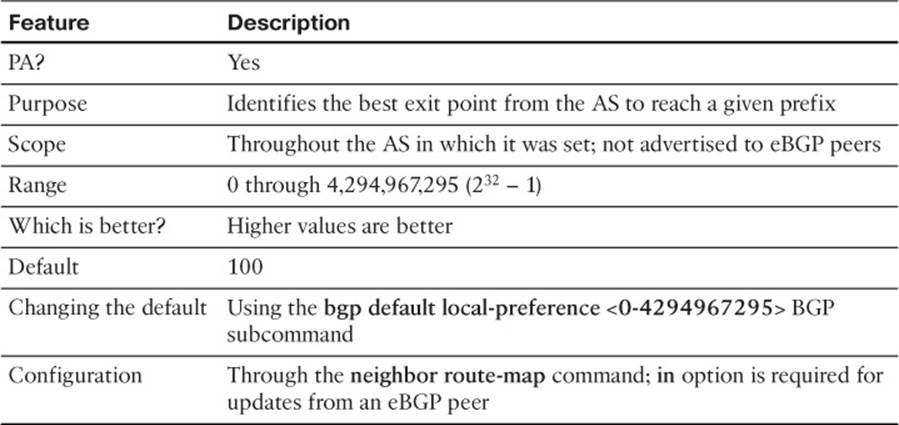
Table 14-7 Key Features of Local_Pref
Note
For those of you memorizing using the N WLLA OMNI mnemonic, Local_Pref is the first L in WLLA.
Sample Internetwork Used in the Local_Pref and AS_Path Length Examples
Figure 14-14 shows a sample internetwork used to demonstrate setting both Local_Pref, and later, AS_Path length. The figure shows a single enterprise with two Internet-connected routers. A full iBGP mesh exists with these two routers plus two routers internal to the enterprise. Two eBGP neighborships exist, one with ISP1 and one with ISP3. (Note in particular that unlike Figure 14-12, E1 does not have a neighborship with Router I3-1 in this case.) The following design requirements have already been met by the initial configuration in all routers shown in the figure:
![]() E1 and I1-1 use loopback IP addresses (11.11.11.11 and 1.1.1.1) for their neighborship.
E1 and I1-1 use loopback IP addresses (11.11.11.11 and 1.1.1.1) for their neighborship.
![]() E2 and I3-1 use interface IP addresses for their neighborship.
E2 and I3-1 use interface IP addresses for their neighborship.
![]() None of the routers have attempted to change any settings that can impact the choice of best path, and Weight settings in the previous examples have been removed.
None of the routers have attempted to change any settings that can impact the choice of best path, and Weight settings in the previous examples have been removed.
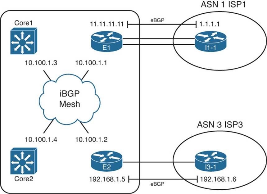
Figure 14-14 Sample Internetwork for BGP Local_Pref and AS_Path Length Examples
As with the Weight example, both ISPs advertise the same five prefixes, with different AS_Paths, so that the routers have some prefixes to manipulate. Figure 14-15 shows five such prefixes that both ISPs advertise to E1 and E2. Note that this example network uses the same five prefixes, prefix lengths, and AS_Path values as the previous Weight examples in this chapter.
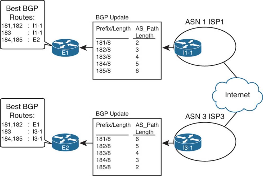
Figure 14-15 Prefixes and AS_Path Lengths Used in Upcoming Examples
Before showing the example of how to set the Local_Pref and how it impacts the routes, it is helpful to look at the best BGP routes on the enterprise routers before any PAs have been changed. Example 14-19 shows the relevant BGP table entries on E1, E2, and Core1 with no attempt to influence E1’s choice of best path. The best path for four of the five prefixes will be obvious, but the output listed in the commands requires some review. Prefixes 181.0.0.0/8 and 182.0.0.0/8 have a shorter AS_Path through ISP1, so E1 and E2 will agree that E1’s path, through ISP1, is best. Similarly, 184.0.0.0/8 and 185.0.0.08 have a shorter AS_Path through ISP3, so both E1 and E2 agree that E2’s path is best for these prefixes. Again, 183.0.0.0/8 ties on AS_Path length.
Example 14-19 BGP Tables on E1, E2, and Core1, with No Changes to Settings That Affect Best Path
! First, on router E1
E1# show ip bgp 176.0.0.0/4 longer-prefixes
BGP table version is 15, local router ID is 128.107.9.1
Status codes: s suppressed, d damped, h history, * valid, > best, i - internal,
r RIB-failure, S Stale
Origin codes: i - IGP, e - EGP, ? - incomplete
Network Next Hop Metric LocPrf Weight Path
*> 181.0.0.0/8 1.1.1.1 0 0 1 1811 i
*> 182.0.0.0/8 1.1.1.1 0 0 1 2 1822 i
* i183.0.0.0/8 10.100.1.2 0 100 0 3 2 50 1833 i
*> 1.1.1.1 0 0 1 2 50 1833 i
*>i184.0.0.0/8 10.100.1.2 0 100 0 3 2 1844 i
* 1.1.1.1 0 0 1 2 50 51 1844 i
*>i185.0.0.0/8 10.100.1.2 0 100 0 3 1855 i
* 1.1.1.1 0 0 1 2 50 51 52 1855 i
! Next, on router E2
E2# show ip bgp 176.0.0.0/4 longer-prefixes
! legend omitted for brevity
Network Next Hop Metric LocPrf Weight Path
*>i181.0.0.0/8 10.100.1.1 0 100 0 1 1811 i
* 192.168.1.6 0 0 3 2 50 51 52 1811 i
*>i182.0.0.0/8 10.100.1.1 0 100 0 1 2 1822 i
* 192.168.1.6 0 0 3 2 50 51 1822 i
* i183.0.0.0/8 10.100.1.1 0 100 0 1 2 50 1833 i
*> 192.168.1.6 0 0 3 2 50 1833 i
*> 184.0.0.0/8 192.168.1.6 0 0 3 2 1844 i
*> 185.0.0.0/8 192.168.1.6 0 0 3 1855 i
! Next, on router Core1
Core1# show ip bgp 176.0.0.0/4 longer-prefixes
! legend omitted for brevity
Network Next Hop Metric LocPrf Weight Path
*>i181.0.0.0/8 10.100.1.1 0 100 0 1 1811 i
*>i182.0.0.0/8 10.100.1.1 0 100 0 1 2 1822 i
*>i183.0.0.0/8 10.100.1.1 0 100 0 1 2 50 1833 i
* i 10.100.1.2 0 100 0 3 2 50 1833 i
*>i184.0.0.0/8 10.100.1.2 0 100 0 3 2 1844 i
*>i185.0.0.0/8 10.100.1.2 0 100 0 3 1855 i
First, pay close attention to the LocPrf column of output in the example. This column lists the Local_Pref settings of each route. Some list a (default) value of 100, and some list nothing. As it turns out, because Updates received from eBGP peers do not include the Local_Pref PA, Cisco IOS lists a null value for Local_Pref for eBGP-learned routes by default. However, Updates from iBGP peers do include the Local_Pref. Because this network does not have any configuration that attempts to set Local_Pref yet, the routers advertise their default Local_Pref value of 100 over the iBGP connections.
Also note that when comparing the output on both E1 and E2, the output lists a single eBGP route, but not the alternative iBGP route through the other Internet-connected router in the enterprise. For example, E2 lists a single route for 184.0.0.0/8 and 185.0.0.0/8, through I3-1 (192.168.1.6). The reason that E2 does not list an alternative route through E1 is that E1’s best route for these prefixes, as seen near the top of the example, is E1’s iBGP-learned route through E2 (10.100.1.2). BGP does not allow a router to advertise iBGP-learned routes to iBGP peers, so E1 will not advertise routes for 184.0.0.0/8 or 185.0.0.0/8 to Router E2.
Finally, for prefix 183.0.0.0/8, both E1 and E2 tie on the AS_Path length. In this case, all best-path choices tie until Step 7, which prefers eBGP routes over iBGP routes. E1 prefers its eBGP route for 183.0.0.0/8 through ISP1’s Router I1-1, and E2 prefers its eBGP route through ISP3’s Router I3-1.
Setting the BGP Local_Pref Using a Route Map
To set the Local_Pref, a router can use the neighbor neighbor-ip route-map in BGP subcommand. Typically, a router uses this command with the inbound direction for routes received from eBGP peers. Then, with no additional configuration required, the router then advertises the Local_Pref to any iBGP peers.
To show the Local_Pref configuration and results, start with the sample network shown in the previous section. The configuration will now be changed to set the Local_Pref for two different prefixes for Updates received on E1 from I1-1, as shown in Figure 14-16. Note that the figure reinforces the idea that BGP does not include the Local_Pref PA in eBGP Updates but will in iBGP Updates.
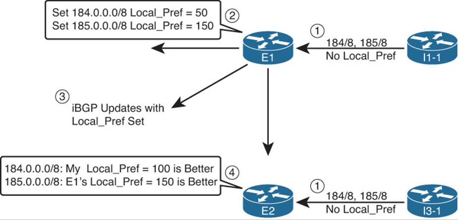
Figure 14-16 Example Local_Pref Settings for the Upcoming Example
The figure shows a series of steps, as follows:
Step 1. I1-1 and I3-1 advertise the prefixes into the enterprise but with no Local_Pref set, because the connections are eBGP peers.
Step 2. E1 sets the Local_Pref for routes learned from I1-1: 184.0.0.0/8 (50) and 185.0.0.0/8 (150).
Step 3. E1 includes the Local_Pref settings in its iBGP Updates to Core1, Core2, and E2.
Step 4. E2 realizes that E1’s route for 185.0.0.0/8, Local_Pref 150, is better than E2’s eBGP route for this prefix, which E2 assigned default Local_Pref 100. Conversely, E1’s advertised route for 184.0.0.0/8, Local_Pref 50, is worse than E2’s eBGP route for that same prefix, with the assigned default Local_Pref of 100.
Example 14-20 shows the configuration on Router E1 to assign the Local_Pref values shown in Figure 14-16. The example also shows the results on E1 and E2. Note that the configuration differs only slightly as compared with the configuration for administrative Weight as shown in Example 14-17, the only substantive difference being the set local-preference route map command rather than the set weight command.
Example 14-20 Configuring Local_Pref on Router E1 (Step 2 per Figure 14-16)
E1# show running-config
! only pertinent portions shown
ip prefix-list match-184 seq 5 permit 184.0.0.0/8
!
ip prefix-list match-185 seq 5 permit 185.0.0.0/8
!
route-map set-LP-150 permit 10
match ip address prefix-list match-185
set local-preference 150
!
route-map set-LP-150 permit 15
match ip address prefix-list match-184
set local-preference 50
!
route-map set-LP-150 permit 20
!
router bgp 11
neighbor 1.1.1.1 route-map set-LP-150 in
! The clearing of BGP neighbor I1-1 is done next, but not shown.
! Next, E1's Updated BGP Table
E1# show ip bgp 176.0.0.0/4 longer-prefixes
BGP table version is 29, local router ID is 128.107.9.1
Status codes: s suppressed, d damped, h history, * valid, > best, i - internal,
r RIB-failure, S Stale
Origin codes: i - IGP, e - EGP, ? - incomplete
Network Next Hop Metric LocPrf Weight Path
*> 181.0.0.0/8 1.1.1.1 0 0 1 1811 i
*> 182.0.0.0/8 1.1.1.1 0 0 1 2 1822 i
* i183.0.0.0/8 10.100.1.2 0 100 0 3 2 50 1833 i
*> 1.1.1.1 0 0 1 2 50 1833 i
*>i184.0.0.0/8 10.100.1.2 0 100 0 3 2 1844 i
* 1.1.1.1 0 50 0 1 2 50 51 1844 i
*> 185.0.0.0/8 1.1.1.1 0 150 0 1 2 50 51 52 1855 i
E1# show ip bgp 185.0.0.0/8
BGP routing table entry for 185.0.0.0/8, version 7
Paths: (1 available, best #1, table Default-IP-Routing-Table)
Advertised to update-groups:
1
1 2 50 51 52 1855, (received & used)
1.1.1.1 from 1.1.1.1 (1.1.1.1)
Origin IGP, metric 0, localpref 150, valid, external, best
! The next output occurs on router E2
E2# show ip bgp 185.0.0.0/8 longer-prefixes
! heading lines omitted
Network Next Hop Metric LocPrf Weight Path
*>i185.0.0.0/8 10.100.1.1 0 150 0 1 2 50 51 52 1855 i
* 192.168.1.6 0 0 3 1855 i
Example 14-20’s output shows E1’s BGP table entries, now with updated Local_Pref values as compared with Example 14-19. E1 now uses its eBGP route, Next_Hop 1.1.1.1, for prefix 185.0.0.0/8 because of the higher Local_Pref.
The end of the example shows E2 with two possible routes for 185.0.0.0/8. The following list outlines E2’s BGP best-path logic in this case:
Step 0. The two routes both have reachable Next_Hop IP addresses.
Step 1. Both have Weight 0 (tie).
Step 2. The iBGP route through 10.100.1.1 (E1) has a bigger (better) Local_Pref (150 versus 100) than the route through 192.168.1.6 (I3-1), so it is the better route.
Also, note that both the show ip bgp longer-prefixes command’s briefer output, and the show ip bgp 185.0.0.0/8 commands more verbose output, both identify the Local_Pref value. However, the longer command output does not list the Weight value.
IP Routes Based on BGP Best Paths
Some of the complexity related to BGP occurs around the BGP functions created by BGP PAs, including their use by the best-path algorithm. When the BGP best-path algorithm has gotten through this complexity and chosen a best route for a prefix, the router then tries to add that route to the IP routing table. However, rather than add the BGP route to the IP routing table directly, BGP actually gives that best BGP route to another process for consideration: the Cisco IOS Routing Table Manager (RTM).
The Cisco IOS RTM chooses the best route among many competing sources. For example, routes can be learned by an IGP, BGP, or even as connected or static routes. Cisco IOS collects the best such route for each prefix and feeds those into the RTM function. The RTM then chooses the best route. Figure 14-17 shows the general idea.
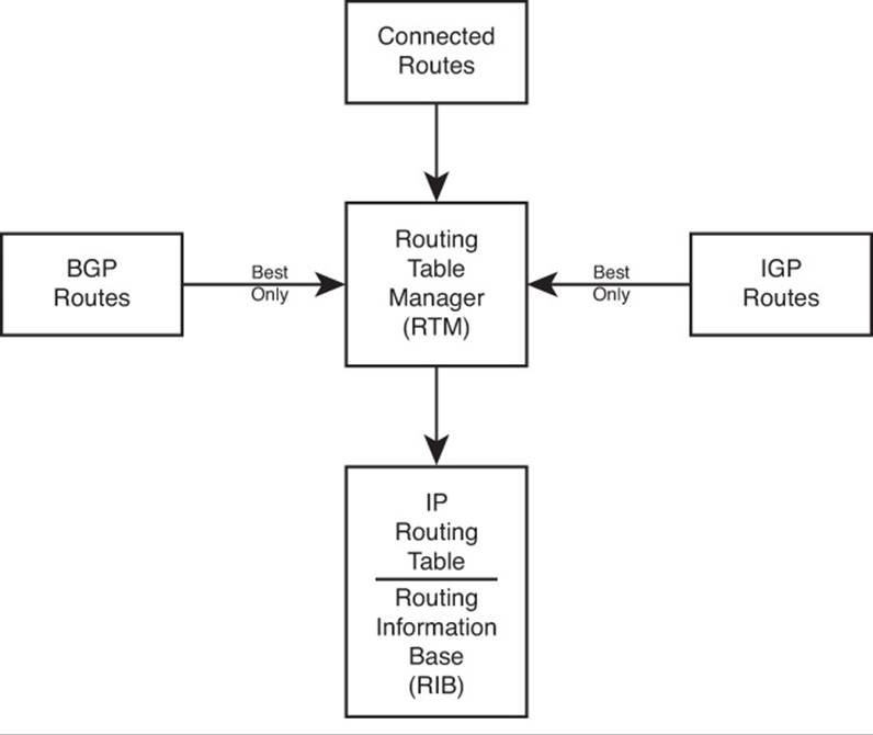
Figure 14-17 Routing Table Manager Concept
Among its tasks, RTM uses the concept of administrative distance (AD) to choose the best route among these different sources. Table 14-8 provides a reminder (and a reference) for the default AD of various route information sources. However, focus on the eBGP and iBGP AD values.
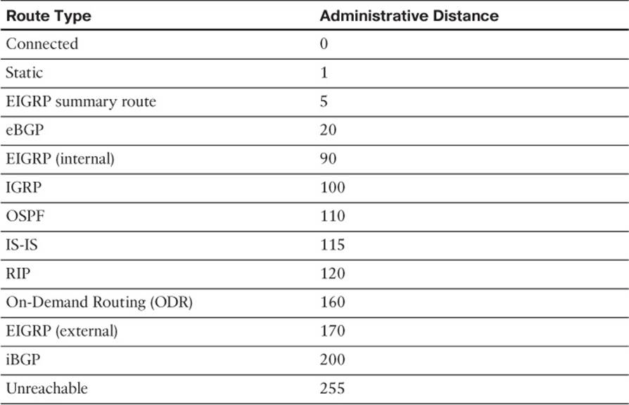
Table 14-8 Default Administrative Distances
For the most part, an enterprise router should not see cases in which a prefix learned with BGP has also been learned as a connected or IGP-learned route. (Conversely, these issues occur more often when implementing MPLS VPNs with BGP/IGP redistribution.) However, it can happen, and when it does, the show ip bgp rib-failures command can be helpful. This command lists routes for which BGP has chosen the route as best, but the RTM function has not placed the route into the Routing Information Base (RIB), which is simply another name for the IP routing table.
Example of a BGP RIB Failure
To show an example of a RIB failure, imagine that an enterprise engineer needs to do some testing, so the engineer just picks an IP address range to use. The engineer tries to avoid problems by not using network 10.0.0.0, which is used throughout the enterprise. Rather than choosing another private network, the engineer chooses public range 185.0.0.0/8. After changing the lab configuration repeatedly, a route for 185.0.0.0/8 leaks into the OSPF topology database.
Keep in mind that at the end of the previous example, E1 had chosen its eBGP route for 185.0.0.0/8 as its best route, and E2 had chosen its iBGP route as its best route for 185.0.0.0/8. Example 14-21 shows the results, based on RTM’s comparisons of the AD values.
Example 14-21 Example with the RTM and RIB Failures
! First, E1's IP Routing table for 185.0.0.0/8
E1# show ip route 185.0.0.0 255.0.0.0 longer-prefixes
Codes: C - connected, S - static, R - RIP, M - mobile, B - BGP
D - EIGRP, EX - EIGRP external, O - OSPF, IA - OSPF inter area
N1 - OSPF NSSA external type 1, N2 - OSPF NSSA external type 2
E1 - OSPF external type 1, E2 - OSPF external type 2
i - IS-IS, su - IS-IS summary, L1 - IS-IS level-1, L2 - IS-IS level-2
ia - IS-IS inter area, * - candidate default, U - per-user static route
o - ODR, P - periodic downloaded static route
Gateway of last resort is 1.1.1.1 to network 0.0.0.0
B 185.0.0.0/8 [20/0] via 1.1.1.1, 00:25:11
! Next, E2's IP Routing table
E2# show ip route 185.0.0.0 255.0.0.0 longer-prefixes
! Legend omitted for brevity
Gateway of last resort is 192.168.1.6 to network 0.0.0.0
O 185.0.0.0/8 [110/2] via 10.1.1.77, 00:15:44, FastEthernet0/0
E2# show ip bgp rib-failure
Network Next Hop RIB-failure RIB-NH Matches
185.0.0.0/8 10.100.1.1 Higher admin distance n/a
The first command shows that E1, with an eBGP route, actually adds its route to the IP routing table. The route lists a code of B, meaning BGP. The output lists the eBGP default AD of 20, which is a better default AD than OSPF’s 110. RTM added this BGP route to the IP routing table on E1 because of eBGP’s better AD.
E2 currently lists its iBGP route through E1 as its current best BGP route for 185.0.0.0/8 because of the higher Local_Pref configured in Example 14-20. However, after giving this route to the RTM, RTM instead chose the lower-AD OSPF route (AD 110) rather than the higher-AD iBGP route (AD 200).
Finally, the show ip bgp rib-failure command lists one line for each best BGP route that the RTM does not place into the IP routing table. In this case, this command on Router E2 lists the route for 185.0.0.0/8, with the reason listed.
BGP and the maximum-paths Command
Like the IGP protocols, BGP supports the maximum-paths number-of-paths subcommand, but BGP uses significantly different logic than the IGPs. Unlike the IGP routing protocols, BGP truly needs to pick one route, and only one route, as the best path for a given prefix/length. In effect, the BGP best-path algorithm already breaks the ties for “best” route for each prefix. Therefore, from BGP’s perspective, one route for each prefix is always best.
BGP does allow multiple BGP routes for a prefix to be considered to tie, at least for the purpose of adding multiple routes to the IP routing table. The conditions are as follows:
If the BGP best-path algorithm does not choose a best path by Step 8 (per the numbering in this book), the routes which still tie for being best path will be allowed into the IP routing table, up to and including the number defined by the BGP maximum-paths number-of-pathsrouter subcommand.
The section “Overview of the BGP Best-Path Algorithm,” earlier in this chapter, lists the best-path steps, including the tiebreaker steps that allow routes to be considered by the maximum-paths command.
Increasing the Length of the AS_Path Using AS_Path Prepend
Step 4 of the BGP best-path algorithm examines the length of the AS_Path PA. The length of the AS_Path might appear to be obvious: Just add the number of ASNs listed in the AS_Path. However, some BGP features outside the scope of this book actually impact the AS_Path length calculation as well. However, for the purposes of this book, AS_Path length is simply the number of ASNs listed in the AS_Path.
The AS_Path prepend tool gives engineers a means to increase the length of an AS_Path by adding ASNs to the AS_Path, while not impacting the loop-prevention role of the AS_Path PA. By increasing the length of an AS_Path, a route is less likely to become the best route. By adding ASNs that already exist inside a particular route’s AS_Path, the feature does not inadvertently prevent a route from being ignored because of AS_Path loop prevention.
For example, using the design shown most recently in Figures 14-13, 14-14, and 14-15, imagine that the enterprise considers ISP1 to be the better ISP, but it does not want to send all traffic through ISP1. So, the enterprise network engineers could make the following type of implementation choice:
Make the AS_Paths received from ISP3 be two ASNs longer.
By making such a choice, when an AS_Path through ISP1 is better, or when it’s a tie on AS_Path length between ISP1 and ISP3, or when the AS_Path through ISP1 is even slightly longer than through ISP3, the routers can still choose their routes through ISP1. Only when the AS_Path (before prepending) is at least two ASNs shorter through ISP3 can the ISP3 path be chosen.
Note
For those of you memorizing using the N WLLA OMNI mnemonic, AS_Path Length is the A in WLLA.
Figure 14-18 shows the mechanics of how an enterprise router would prepend the AS_Path for routes received by Router E2 from ISP3, namely, Router I3-1. Looking specifically at the route for 185.0.0.0/8, in this case, I3-1 has not changed the AS_Path and advertised the route with AS_Path (3, 1855). At Step 2, Router E2 prepends ASN 3—twice—making the AS_Path length 4. At Step 3, E2 advertises the route to its iBGP peers—peers that might now prefer the other route for this prefix through Router E1.
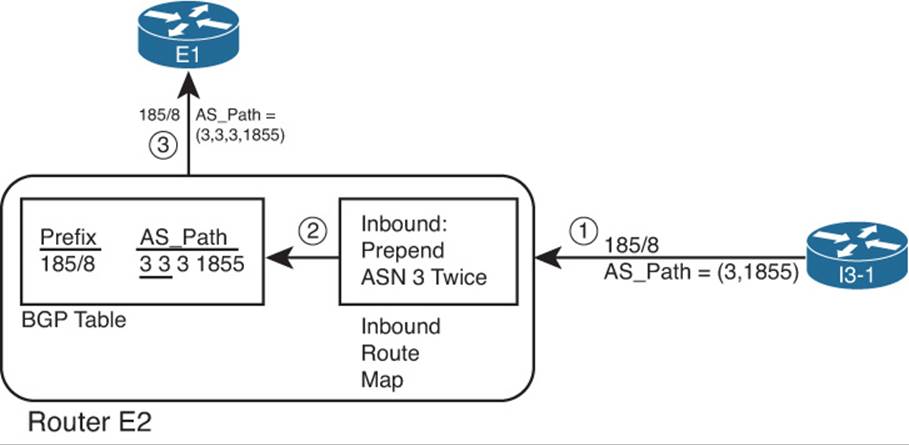
Figure 14-18 Prepending Two ASNs to an AS_Path
The configuration itself requires only a little additional work compared to the other examples. As shown in Figure 14-18, Router E2 could use an inbound route map, using the set as-path prepend 3 3 command to add the two ASN instances. (The router sending the Update, ISP3’s Router I3-1 in this case, could instead use an outbound route map.) Example 14-22 shows the configuration on E2 to add the ASNs at ingress into E2. (Note that all configuration for changing the Weight and Local_Pref, and the extra OSPF route for 185.0.0.0/8 shown in Example 14-20, has been removed before gathering the output in this example.)
Example 14-22 Prepending Additional ASNs to the AS_Path
! First, E2's new configuration
route-map add-two-asns permit 10
set as-path prepend 3 3
router bgp 11
neighbor 192.168.1.6 route-map add-two-asns in
!
! Next, note the AS_Path values all start with 3, 3, 3
E2# show ip bgp 176.0.0.0/4 longer-prefixes
BGP table version is 41, local router ID is 10.100.1.2
Status codes: s suppressed, d damped, h history, * valid, > best, i - internal,
r RIB-failure, S Stale
Origin codes: i - IGP, e - EGP, ? - incomplete
Network Next Hop Metric LocPrf Weight Path
*>i181.0.0.0/8 10.100.1.1 0 100 0 1 1811 i
* 192.168.1.6 0 0 3 3 3 2 50 51 52 1811 i
*>i182.0.0.0/8 10.100.1.1 0 100 0 1 2 1822 i
* 192.168.1.6 0 0 3 3 3 2 50 51 1822 i
*>i183.0.0.0/8 10.100.1.1 0 100 0 1 2 50 1833 i
* 192.168.1.6 0 0 3 3 3 2 50 1833 i
* i184.0.0.0/8 10.100.1.1 0 100 0 1 2 50 51 1844 i
*> 192.168.1.6 0 0 3 3 3 2 1844 i
*> 185.0.0.0/8 192.168.1.6 0 0 3 3 3 1855 i
Note
When using AS_Path prepending, do not prepend just any ASN. BGP still uses the AS_Path for loop avoidance. So, using an ASN already in the AS_Path, like the ASN of the most recently added ASN (for example, ASN 3 in this case), or the local ASN (for example, ASN 11 in this case), makes the most sense.
Although presented here as a tool for influencing outbound routes, AS_Path prepending can also be used to influence the inbound routes.
Influencing an Enterprise’s Inbound Routes with MED
An enterprise has reasonably good control over its outbound IP routes. The engineers can configure BGP to set and react to Weight, Local_Pref, and AS_Path length, manipulating each to choose a different outgoing link or different router through which to forward packets to the Internet.
An enterprise has much less control over inbound routes: routes for packets coming back toward the enterprise. First, these inbound routes exist on routers that the enterprise does not own. Even if an ISP or set of ISPs can be convinced by engineers at the enterprise to make their routes toward an enterprise take a particular path, technical issues can prevent the design from being implemented. In particular, if the enterprise’s public IP address range is summarized, the companies that use addresses in that range might have competing goals. As a result, no policy can be applied to influence the best route.
However, several tools exist that allow some control over the last ASN hop between an ISP and its enterprise customer. This book examines one such tool, called Multi-Exit Discriminator (MED), which originally worked for a dual-homed design—that is, with a single ISP but with multiple links to that ISP. MED was later expanded to support dual-multihomed designs (2+ ASNs, 2+ links), relying on the concept that ISPs would work together. This section examines the dual-homed case, with a single ISP.
MED Concepts
The name Multi-Exit Discriminator actually describes its function to a great degree. With a dual-homed design, at least two links exist between an enterprise and its ISP. The enterprise can announce to the ISP a value (MED) that tells the ISP which path into the enterprise is best. As a result, the ISP can discriminate between the multiple exit points from that ISP to the enterprise.
Because MED lets the enterprise ASN tell just the neighboring ASN which link into the enterprise to use, engineers typically use MED when advertising an enterprise’s public IP address space. Those inbound routes into the enterprise from the ISP typically consist of either one, or a few, public IP address ranges.
For example, consider a new network design as shown in Figure 14-19. In this case, the enterprise uses the same 128.107.0.0/19 public address range used in Chapter 13 and in this chapter. The enterprise connects only to ASN 1 with a total of four physical links and three BGP neighbors.
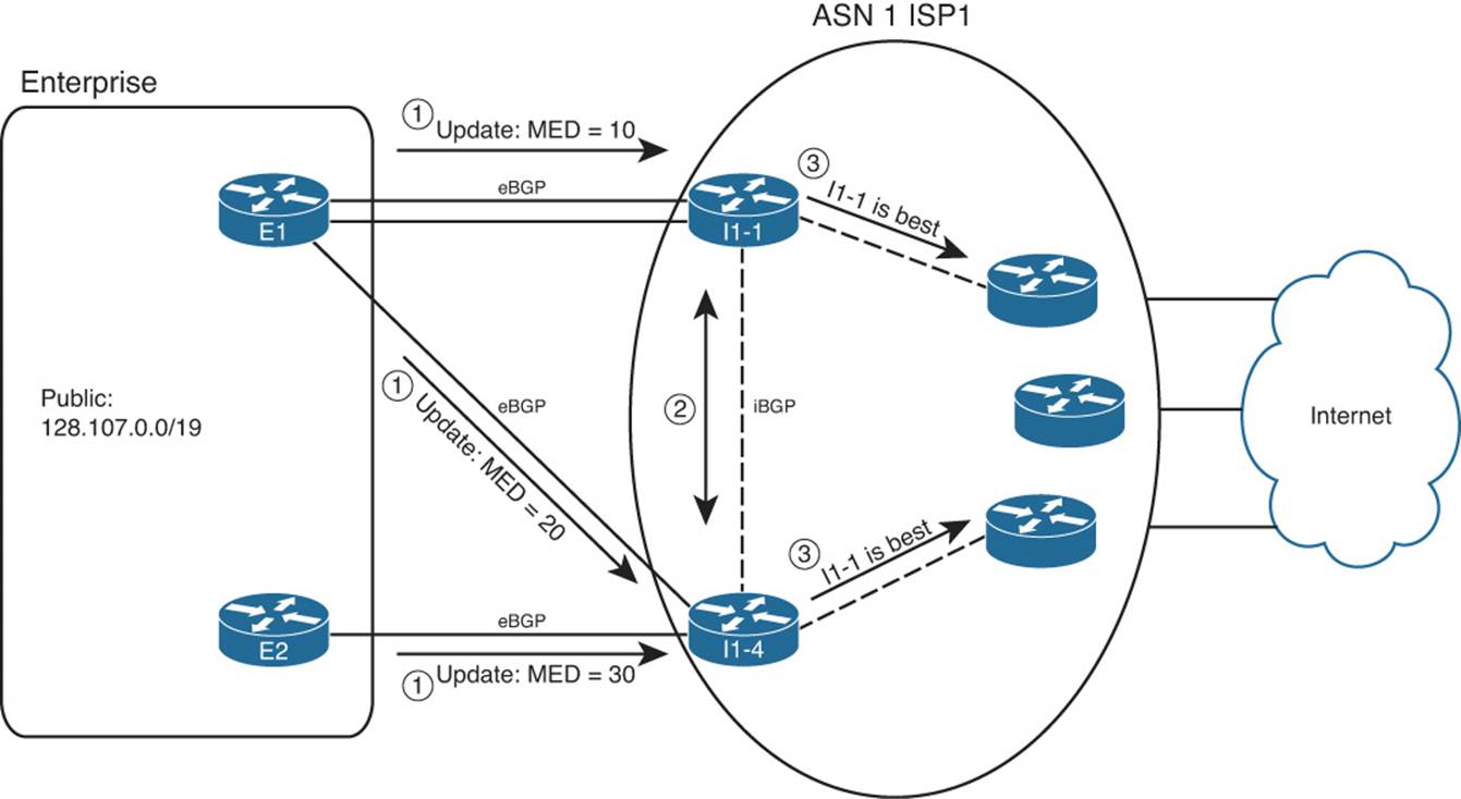
Figure 14-19 Example of Using MED
MED uses smallest-is-best logic. As a result, the figure shows a design in which the enterprise engineer prefers the top BGP neighborship as the best path to use for inbound routes (MED 10), the middle link next (MED 20), and the bottom connection last (MED 30). Following the steps in the figure:
Step 1. E1 and E2 advertise 128.107.0.0/19, setting MED with an outbound route map, to various settings: MED 10 sent by E1 to I1-1, MED 20 sent by E1 to I1-4, and MED 30 sent by E2 to I1-4.
Step 2. I1-1 and I1-4 have an iBGP connection, so they learn each other’s routes and agree as to which route wins based on MED.
Step 3. I1-1 and I1-4 also tell the other routers inside ISP1, causing all inbound traffic to funnel toward Router I1-1.
Note that Routers I1-1 and I1-4 in this example could have chosen a better route based on all the earlier best-path steps. However, a brief analysis of the steps tells us that unless someone makes an effort to override the effects of MED, these routers’ best-path algorithms will use MED. Assuming that the enterprise and ISP agree to rely on MED, the earlier best-path steps should not matter. Here’s why:
Step 1. Weight: Needs to be set locally. Therefore, if relying on MED, the ISP simply chooses to not set the Weight for received Updates from the enterprise.
Step 2. Local_Pref: Again, this takes overt effort to match and set the Local_Pref. If relying on MED, the ISP simply chooses to not set the Local_Pref.
Step 3. Locally injected? All these public routes from the enterprise will be learned with eBGP and not locally injected.
Step 4. AS_Path length: All such routes on the ISP routers should list one ASN—the enterprise’s ASN—so all should tie on this point.
Step 5. Origin: Whatever the Origin is (i, e, or ?), it should tie.
Step 6. MED: None of the other steps determined the best route. Therefore, MED now takes effect.
Table 14-9 summarizes the key points about MED.
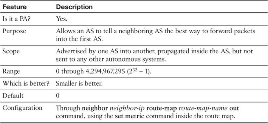
Table 14-9 Key Features of MED
Note
For those of you memorizing using the N WLLA OMNI mnemonic, MED is the M in OMNI.
MED Configuration
MED configuration usually occurs on the routers in the AS that want to control inbound routes from the neighboring AS. As such, in the example design shown in Figure 14-19, Routers E1 and E2 would configure MED. Example 14-23 shows E1’s configuration.
Example 14-23 MED Configuration on Router E1
route-map set-med-to-I1-1 permit 10
match ip address prefix-list only-public
set metric 10
!
route-map set-med-to-I1-4 permit 10
match ip address prefix-list only-public
set metric 20
!
ip prefix-list only-public permit 128.107.0.0/19
!
router bgp 11
neighbor 1.1.1.1 route-map set-med-I1-1 out
neighbor 192.168.1.2 route-map set-med-I1-4 out
Both the configuration and the show ip bgp command output refer to MED as metric. Note that the route map in Example 14-23 uses the set metric command, rather than set med (which does not exist). And as shown in I1-1’s output for the show ip bgp command in Example 14-24, the output lists MED under the heading metric. Specifically, note that even the show ip route command lists the MED value in brackets as the metric for the BGP route.
Example 14-24 BGP Table and IP Routing Table on Router I1-1
I1-1# show ip bgp 128.107.0.0/19
BGP routing table entry for 128.107.0.0/19, version 13
Paths: (1 available, best #1, table Default-IP-Routing-Table)
Flag: 0x820
Not advertised to any peer
11, (aggregated by 11 128.107.9.1), (received & used)
11.11.11.11 from 11.11.11.11 (128.107.9.1)
Origin IGP, metric 10, localpref 100, valid, external, atomic-aggregate, best
I1-1# sh ip bgp 128.107.0.0/19 longer-prefixes
BGP table version is 13, local router ID is 1.1.1.1
Status codes: s suppressed, d damped, h history, * valid, > best, i - internal,
r RIB-failure, S Stale
Origin codes: i - IGP, e - EGP, ? - incomplete
Network Next Hop Metric LocPrf Weight Path
*> 128.107.0.0/19 11.11.11.11 10 0 11 i
I1-1# show ip route 128.107.0.0 255.255.224.0 longer-prefixes
! Legend omitted for brevity
Gateway of last resort is not set
128.107.0.0/19 is subnetted, 1 subnets
B 128.107.0.0 [20/10] via 11.11.11.11, 00:02:18
Exam Preparation Tasks
Planning Practice
The CCNP ROUTE exam expects test takers to review design documents, create implementation plans, and create verification plans. This section provides some exercises that can help you to take a step back from the minute details of the topics in this chapter so that you can think about the same technical topics from the planning perspective.
For each planning practice table, simply complete the table. Note that any numbers in parentheses represent the number of options listed for each item in the solutions in Appendix F, “Completed Planning Practice Tables.”
Design Review Table
Table 14-10 lists several design goals related to this chapter. If these design goals were listed in a design document, and you had to take that document and develop an implementation plan, what implementation options come to mind? You should write a general description; specific configuration commands are not required.
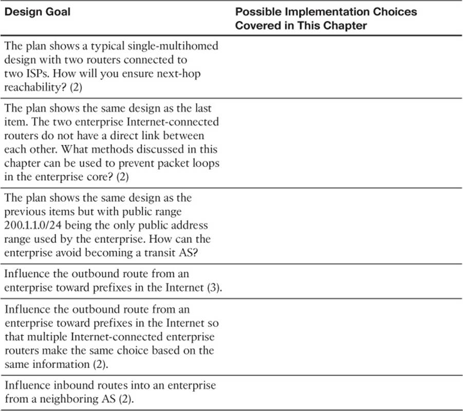
Table 14-10 Design Review
Implementation Plan Peer Review Table
Table 14-11 shows a list of questions that others might ask, or that you might think about, during a peer review of another network engineer’s implementation plan. Complete the table by answering the questions.
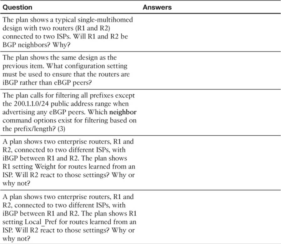
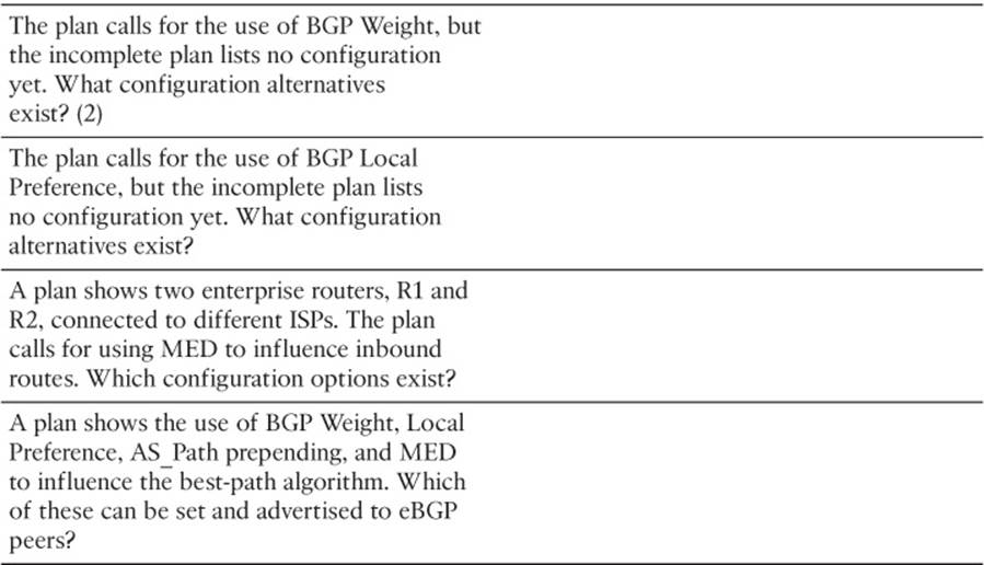
Table 14-11 Notable Questions from This Chapter to Consider During an Implementation Plan Peer Review
Create an Implementation Plan Table
To practice skills useful when creating your own implementation plan, list in Table 14-12 all configuration commands related to the configuration of the following features. You might want to record your answers outside the book and set a goal to complete this table (and others like it) from memory during your final reviews before taking the exam.
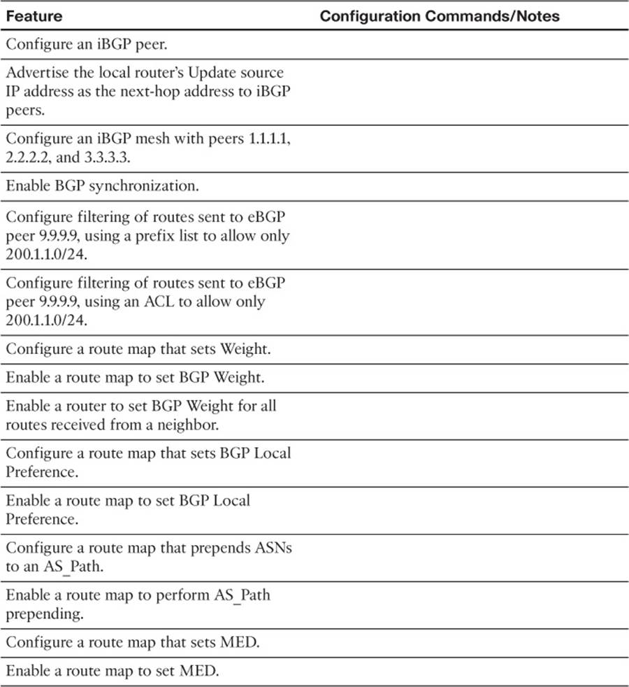
Table 14-12 Implementation Plan Configuration Memory Drill
Choosing Commands for a Verification Plan Table
To practice skills useful when creating your own verification plan, list in Table 14-13 all commands that supply the requested information. You might want to record your answers outside the book and set a goal to complete this table (and others like it) from memory during your final reviews before taking the exam.
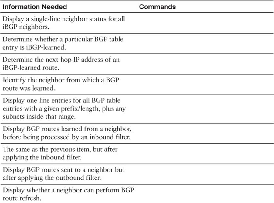
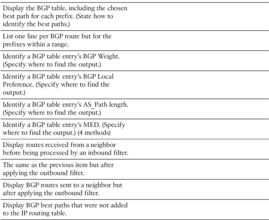
Table 14-13 Verification Plan Memory Drill
Note
Some of the entries in this table may not have been specifically mentioned in this chapter but are listed in this table for review and reference.
Review All the Key Topics
Review the most important topics from inside the chapter, noted with the Key Topic icon in the outer margin of the page. Table 14-14 lists a reference of these key topics and the page numbers on which each is found.
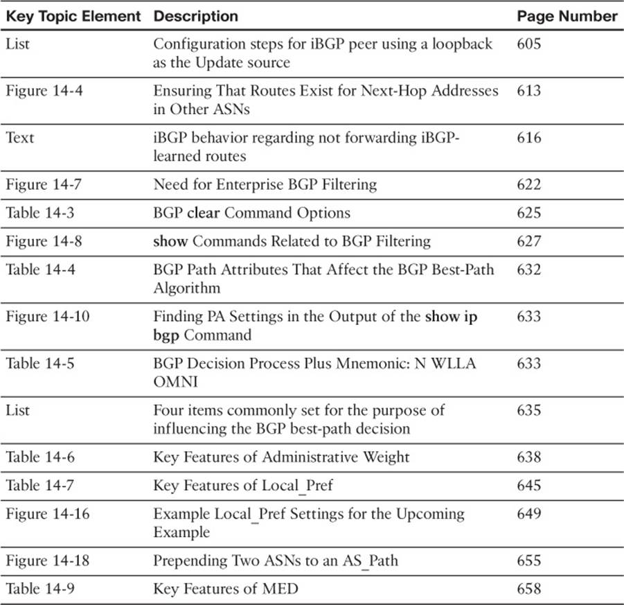
Table 14-14 Key Topics for Chapter 14
Complete the Tables and Lists from Memory
Print a copy of Appendix D, “Memory Tables,” (found on the CD) or at least the section for this chapter, and complete the tables and lists from memory. Appendix E, “Memory Tables Answer Key,” also on the CD, includes completed tables and lists to check your work.
Define Key Terms
Define the following key terms from this chapter, and check your answers in the glossary.
BGP synchronization
iBGP Mesh
next-hop self
BGP soft reset
BGP hard reset
BGP Weight
Local Preference
AS_Path Prepending
Multi-Exit Discriminator
best-path algorithm
Routing Table Manager
RIB failure
path attribute
All materials on the site are licensed Creative Commons Attribution-Sharealike 3.0 Unported CC BY-SA 3.0 & GNU Free Documentation License (GFDL)
If you are the copyright holder of any material contained on our site and intend to remove it, please contact our site administrator for approval.
© 2016-2026 All site design rights belong to S.Y.A.